HEURISTIC APPROACH FOR MULTI QUERY OPTIMIZATION

(1)

Available Online at www.ijpret.com 1100

INTERNATIONAL JOURNAL OF PURE AND

APPLIED RESEARCH IN ENGINEERING AND

TECHNOLOGY

A PATH FOR HORIZING YOUR INNOVATIVE WORK

HEURISTIC APPROACH FOR MULTI QUERY OPTIMIZATION

PROF. A. D. ISALKAR1_{, PROF. M. K. POPAT}2

1. Department of Information Technology, DMIETR, Wardha, India. 2. Department of Computer Science, SGBAU, JDIET, Yavatmal, India.

Accepted Date: 05/03/2015; Published Date: 01/05/2015

Abstract: Now a day, it is very common to see that complex queries are being vastly used in the real time database applications. These complex queries often have a lot of common sub-expressions, either within a single query or across multiple such queries run as a batch. Multi-query optimization aims at exploiting common sub-expressions to reduce evaluation cost. Multi-query optimization has often been viewed as impractical, since earlier algorithms were exhaustive, and explore a doubly exponential search space. This work demonstrates that multi-query optimization using heuristics is practical, and provides significant benefits. The cost-based heuristic algorithms: basic Volcano-SH and Volcano-RU, which are based on simple modifications to the Volcano search strategy. The algorithms are designed to be easily added to existing optimizers. The study shows that the presented algorithms provide significant benefits over traditional optimization, at a very acceptable overhead in optimization time.

Keywords: Heuristics, Volcano-SH, Volcano-RU

Corresponding Author: PROF. A. D. ISALKAR

Access Online On:

www.ijpret.com

How to Cite This Article:

A. D. Isalkar, IJPRET, 2015; Volume 3 (9): 1100-1111

(2)

INTRODUCTION

The main idea of Multi-Query Optimization is to optimize the set of queries together and execute the common operation once. Complex queries are becoming commonplace, with the growing use of decision support systems.

Approaches to Query Optimization:

 Systematic query optimization.

 Heuristic query optimization.

 Semantic query optimization.

1.1Systematic query optimization

In systematic query optimization, the system estimates the cost of every plan and then chooses the best one. The best cost plan is not always universal since it depends on the constraints put on data. For example, joining on a primary key may be done more easily than joining on a foreign key since primary keys are always unique and therefore after getting a joining partner, there is no other key expected. The system therefore breaks out of the loop and hence does not scan the whole table. Though in many cases efficient, it is a time wasting practice and therefore sometimes it can be done away with .The costs considered in systematic query optimization include access cost to secondary storage, storage cost, computation cost for intermediate relations and communication costs.

1.2Heuristic query optimization

In the heuristic approach, the operator ordering is used in a manner that economizes the resource usage but conserving the form and content of the query output. The principle aim is to:

(i) Set the size of the intermediate relations to the minimum and increase the rate at which

the intermediate relation size tend towards the final relation so as to optimize memory.

(ii) Minimize on the amount of processing that has to be done on the data without

(3)

1.3Semantic query optimization:

This is a combination of Heuristic and Systematic optimization. The constraints specified in the database schema can be used to modify the procedures of the heuristic rules making the optimal plan selection highly creative. This leads to heuristic rules that are locally valid though cannot be taken as rules of the thumb.

2. Multi Query Processing

In multi query optimization, queries are optimized and executed in batches. Individual queries are transformed into relational algebra expressions and are represented as graphs the graphs are created in such away that:

(i) Common sub-expressions can be detected and unified;

(ii) Related sub-expressions are identified so that the more encompassing sub expression is executed and the other sub-expressions are derived from it. Before studying how exactly optimizer works, or how exactly the optimization takes place, we need to first understand where this phase of optimization is implemented in the execution of a query. For that we have to take a brief look on query processing.

Query processing refers to the range of activities involved in extracting the data from database. The activities include transformation of queries in high level database languages into expressions that can be used at physical level of the file system, a variety of query optimizing transformations and actual evaluation of queries.

Referring to the fig the basic steps involved in the query processing are

1) Parsing and translation

2) Optimization

3) Evaluation

(4)

Available Online at www.ijpret.com 1103 Before query processing can begin, the system must translate a query into a usable form. A language such as SQL is suitable for human use, but is ill-suited to be the system’s internal representation of a query. A more suitable internal representation is one based on the extended relational algebra.

Thus, the first action the system must take in query processing is to translate a given query in its internal form. This translation process is similar to the work performed by the parser of a compiler. In generating the internal form of the query, the system uses parsing techniques. The parser used in this query checks the syntax of the query. It verifies that the names of relations appearing in the query as those really present in the database and so on. Thus after constructing the parse tree representation of a query, it translates into the relational algebra expression.

After this, the optimizer comes into play. It takes the relational algebra expression as the input from parser. By applying a suitable optimizing algorithm, it finds out the best plan among the various plans possible. The best plan is nothing but the plan requiring minimum cost for its execution. This plan is provided as the input for further processing.

Finally, the query evaluation engine takes this plan as input, executes it and returns the output of the query. The output is nothing but the specified number of tuples satisfying that query.

Thus, the above figure represents exact location in the whole query processing where the optimizer works.

Generation of optimal global queries is not necessarily done on individual optimal plans. It is done on the group of them. This leads to a large sample space from which the composite optimal plan has to be got. For example, if for four relations A,B, C, and D there are two queries

whose optimal states are Q1 = (A⋈B)⋈C and Q2= (B ⋈ C) ⋈D with execution costs e1 and e2

respectively, the total cost is e1 + e2.Though these queries are individually optimal, the sum is

not necessarily optimal. The query Q1 for example can be rearranged to an individually

non-optimal state Q’ = A⋈ (B⋈C) whose cost, say E1 is greater than e1. The combination of Q’ and

Q2may make a more optimal plan globally at run time in case they cooperate. Since there is a

common expression (B⋈C), it can be executed once and the result shared by the two queries.

This leads to a cost of E1+ e2 –E2where E2 is the cost of evaluating (B⋈C) which can be less

(5)

Available Online at www.ijpret.com 1104 strategy therefore needs to be efficient enough to be cost effective. Though this approach can lead to a lot of improvement on the efficiency of a query, it may still have some bottlenecks that have to be overcome if a global state is at all times to be achieved. The bottlenecks include:-

(a) the cost of Q’ may be too high that the sum of the independent optimal states is still the global optimal state;

(b) There may be no possibility at all to have sharable components and therefore a search for sharable components is wastage of resources.

(c) The new query plans may have a lower resource requirement than the previous one but when the resources taken to identify the plan (search cost) take on more resources than the tradeoff hence no net saving on resources.

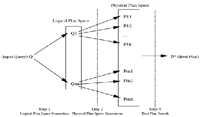
3. Model of a cost-based query optimizer

Figure 2: Overview of Cost-based Query Optimization

Figure gives an overview of the optimizer. Given the input query, the optimizer works in three distinct

Steps:

3.1. Generate all the semantically equivalent rewritings of the input query.

In Figure Q1,………,Qm are the various rewritings of the input query Q. These rewritings recreated by applying “transformations” on different parts of the query; a transformation gives an alternative semantically equivalent way to compute the given part. For example, consider

(6)

Available Online at www.ijpret.com 1105 equivalent to (C⋈B), giving (A⋈ (C⋈B)) as a rewriting. An issue here is how to manage the application of the transformation so as to guarantee that all rewritings of the query possible using the given set of transformations are generated, in as efficient way as possible. For even moderately complex queries, the number of possible rewritings can be very large. So, another issue is how to efficiently generate and compactly represent the set of rewritings.

3.2. Generate the set of executable plans for each rewriting generated in the first step.

Each rewriting generated in the first step serves as a template that defines the order in which

the logical operations (selects, joins, and aggregates) are to be performed – how these operations are to be executed is not fixed. This step generates the possible alternative execution plans for the rewriting.

For example, the rewriting (A⋈ (C⋈B)) specifies that A is to be joined with the result of joining C with B. Now, suppose the join implementations supported are nested-loops-join, merge-join and hash-join. Then, each of the two joins can be performed using any of these three implementations, giving nine possible executions of the given rewriting. In Figure P11,……., P1k are the k alternative execution plans for the rewritingQ1, and Pm1,…., Pmn are the n alternative execution plans for Qm. The issue here, again, is how to efficiently generate the plans and also how to compactly store the enormous space of query plans.

3.3. Search the plan space generated in the second step for the “best plan”.

Given the cost estimates for the different algorithms that implement the logical operations, the cost of each execution plans is estimated. The goal of this step is to find the plan with the minimum cost. Since the size of the search space is enormous for most queries, the core issue here is how to perform the search efficiently. The Volcano search algorithm is based on top-down dynamic programming (“memorization”) coupled with branch-and-bound.

3.4 Directed Acyclic Graph (Dag)

We present an extensible approach for the generation of DAG-structured query plans. A Logical

Query DAG (LQDAG) is a directed acyclic graph whose nodes can be divided into equivalence nodes and operation nodes; the equivalence nodes have only operation nodes as children and

(7)

4. Heuristic Based Algorithms

4.1 The Basic Volcano Algorithm

This determines the cost of the nodes by using a depth first traversal of the DAG. The cost of operational and equivalence nodes are given

bycost(o) = cost of executing (o) + Σei∈children(o)cost(ei)

and the cost of an equivalence node is given by

cost(e) = in(cost(oi)|o2children(e)

If the equivalence node has no children, then

cost(e) = 0. In case a certain node has to be materialized, then the equation for cost(o) is adjusted to incorporate materialization. For a materialized equivalence node, the minimum between the cost of reusing the node and the cost of recomputing the node is used. The equation therefore becomes

cost(o) = cost of executing (o) + Σei∈children(o)C(ei)

whereC(ei) = cost(ei) if ei!∈ M, and = min(cost(ei), reusecost(ei)) ifei∈ M.

4.2 Volcano Algorithm

PROCEDURE: Volcano(eq)

Input: Root node of Expanded DAG

Output: Optimized plan

(8)

Available Online at www.ijpret.com 1107 Step 2: For every inpEq∈ child (op)

Step 3:Volcano(inpEq)

Step 4:If inpEq∈ leaf node

Step 5:cost(inpEq)= 0

Step 6:cost(op) = cost of executing (op) +∑Cost(inpEq)

Step 7: cost(eq) = min{cost(op)|op ∈ children(eq)}

Step 8: mark op as calculated

4.3 The Volcano SH Algorithm

In Volcano-SH the plan is first optimized using the Basic Volcano algorithm and then creating a pseudo root merges the Basic Volcano best plans. The optimal query plans may have common sub-expressions which need to be materialized and reused.

4.4 The Volcano-RU Algorithm

The Volcano-RU exploits sharing well beyond the optimal plans of the individual queries. Though volcano SH algorithm considers sharing, it does it on only individually optimal plans therefore some sharable components which are in optimal plans are left out. Including sub-optimal states however implies that the sample space of the nodes has to increase. The search algorithm must be able to put it into consideration so that the searching cost is still below the extra savings made.

4.5 Calculation of Cost

(9)

Notation Meaning

V1 Number of pages in relation R1

V2 Number of pages in relation R2

Vr Number of pages in result of joining relation R1 and R2

B Number of pages in memory for the use in buffers

B1 Number of pages in memory for relation R1

B2 Number of pages in memory for relation R2

BR Number of pages in memory for result

Table No. 1 Variable Names with their Meaning

We denote the time taken to perform an operation x as Tx. Each operation is a part of one of the join algorithms, such as transferring a page from disk to memory, or partitioning the content of a page. Table below shows the default values used to calculate the results below, were based on a disk drive with 8KB pages, an average seek time of 16ms, and which rotates at 3600RPM.

Notation Meaning Values

TC Cost of constructing a hash table per page in

memory

0.015

TK Cost of moving the disk head to the page on disk 0.0243

TJ Cost of joining a page with a hash table in

memory

0.015

TT Cost of transferring a page from disk to memory 0.013

Table no. 2 Constant Variables

We assume that the cost of a disk operation, transferring a set of Vx disk pages from disk to memory, or from memory to disk, can be given by

Cx = TK + Vx TT

Using this equation, we can derive the cost of transferring a set of Vx disk pages from disk to memory, or from memory to disk, through a buffer of size Bx. It is given by

CI/O(Vx, Bx) = [Vx/Bx]Tk + VxTT

We assume that the memory based part of the join is based on hashing. That is, a hash table is created from the pages of the outer relation, and the records of the inner relation are joined by hashing against this table to find records to join with.

As described above, the total available memory, B pages, is divided into a set of pages for each

(10)

 The sum of the three buffer areas must not be greater than the available memory:

B1+B2+BR<=B.

 The amount of memory allocated to relation R1 should not exceed the size of relation R1:

1<=B1<=V1.

 The amount of memory allocated to relation R2 should not exceed the size of relation R2:

1<=B2<=V2.

 Some memory must be allocated to the result: BR>=1 if VR>=1.

As described above, V1<=V2, therefore relation R1 is the outer relation. It is read previously once, B1 pages at a time, in [V1/B1] I/O operations. Thus, relation R2 will be read [V1/B1] times, B2 pages at a time. Each pass over relation R2, except the first, reads V2-B2 pages due to the rocking over the relation. The total cost of nest block join is given by-

Cost of transferring a set V1 pages through buffer of size B1:

CRead R1 = CI/O(V1,B1)

Cost of creating Hashed Pages from V1 pages:

CCreate = V1TC

Cost of transferring V2 pages through buffer of size B2:

CRead R2 =CI/O(V2,B2)

Cost of joining each hashed page with V2 pages

CJoin = V2TJ

Cost of Writing back the result into the disk drive:

CWrite RR = CI/O(VR,BR)

Total Cost of Operation:

CNB = CRead R1 + CCreate +CRead R2 + CJoin

(11)

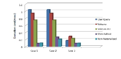
5. RESULTS

The goal of the basic experiments was to quantify the benefits and cost of the three heuristics for multi-query optimization, Volcano-SH, Volcano-RU and Greedy, with plain Volcano-style optimization as the base case. We used the version of Volcano-RU which considers the forward and reverse orderings of queries to find sharing possibilities, and chooses the minimum cost plan amongst the two. Figure 3 shows the comparisons of different algorithms.

Figure 3: Comparison of different algorithms.

6. Future Work

Execution cost is minimum in greedy algorithm and is maximum in Volcano is maximum whereas the optimization cost is maximum in greedy algorithm and minimum in volcano. Thus from this study there is scope in future to combine these two algorithm so that the execution cost of greedy and optimization cost from volcano can be used to evaluate best optimization results for Multi-query optimization.

Since we worked on heuristic based algorithm we just consider only transfer time. For future to work on real time database the seek time and latency time should be considered.

CONCLUSION

(12)

Available Online at www.ijpret.com 1111 Thus we can conclude that the techniques of using Volcano heuristic algorithms are the best approach for Multi-Query-Optimization as compared to other optimization techniques and are practically well implemented. And the comparative study shows that the Volcano, Volcano-SH and Volcano-RU give different optimized results at different cases depending on the logically equivalent queries.

REFERENCES

1. [RSR+99] Prasan Roy, Pradeep Shenoy, Krithi Ramamritham, S. Seshadri, and S. Sudarshan.

Don’t trash your intermediate results, cache ’em. Submitted for publication, October 1999.

2. [RSS96] Kenneth Ross, Divesh Srivastava, and S. Sudarshan. Materialized view maintenance

and integrity constraint checking: Trading space for time. In SIGMOD Intl. Conf. on Management of Data, May 1996.

3. Thomas Neumann and Guido Moerkotte. An effcient framework for order optimization. In

Proceedings of the 20th International Conference on Data Engineering, 30 March - 2 April 2004, Boston, MA, pages 461–472. IEEE Computer Society, 2004.

4. [CCH+98] Latha Colby, Richard L. Cole, Edward Haslam, NasiJazayeri, Galt Johnson, William J.

McKenna, Lee Schumacher, and David Wilhite. Redbrick Vista: Aggregate computation and management. In Intl. Conf.on Data Engineering, 1998.

5. Surajit Chaudhuri, Ravi Krishnamurthy, Spyros Potamianos, And Kyuseok Shim. Optimizing

queries with materialized views. In Intl. Conf. on Data Engineering, Taipei, Taiwan, 1995.

6. Surajit Chaudhuri and Vivek Narasayya. An efficient cost-driven index selection tool for

microsoft SQL Server. In Intl. Conf. Very Large Databases, 1997.

7. [GHRU97] H. Gupta, V. Harinarayan, A. Rajaraman, and J. Ullman. Index selection for olap.In

Intl. Conf. on Data Engineering, Binghampton, UK, April 1997.

8. Arjan Pellenkoft, Cesar A. Galindo-Legaria, and Martin Kersten. The Complexity of