PERFORMANCE EVALUATION OF A WIRELESS SENSOR NETWORK FOR MOBILE AND STATIONARY EVENT CASES CONSIDERING ROUTING EFFICIENCY AND
GOODPUT METRICS
TAO YANG∗, LEONARD BAROLLI†, MAKOTO IKEDA∗, GIUSEPPE DE MARCO‡, AND ARJAN DURRESI§ Abstract. Sensor networks are a sensing, computing and communication infrastructure that are able to observe and respond to phenomena in the natural environment and in our physical and cyber infrastructure. The sensors themselves can range from small passive microsensors to larger scale, controllable weather-sensing platforms. Presently, there are many research works for sensor networks. In our previous work, we built a simulation system for simulation the sensor networks. But, we considered that the event node is stationary in the observation field. However, in many applications the event node may move. For example, in an ecology environment the animals can move randomly. In this work, we investigate how the sensor network performs in the case when the event node moves. We carried out the simulations for lattice topology and TwoRayGround radio model considering AODV and DSR protocols. For the performance evaluation, we considered two metrics: routing efficiency and goodput and we compare the simulation results for two cases: when the event node is mobile and stationary. The simulation results have shown that the routing efficiency for the case of mobile event node is better than the stationary event node using AODV protocol. Also, the goodput for the mobile event node case does not change too much compared with the stationary event case using AODV, but the goodput is not good when the number of nodes is increased.
Key words: sensor network, mobile event, goodput, routing efficiency
1. Introduction. A Wireless Sensor Network (WSN) is a wireless network where the nodes are sensors, that is micro-devices with limited computation capacity and with on-board specific transducers. Recently, we witnessed a lot of research effort towards the optimization of standard communication paradigms for such networks. In fact, the traditional Wireless Network (WN) design has never paid attention to constraints such as the limited or scarce energy of nodes and their computational power. Another aspect which is different from traditional WN is the communication reliability and congestion control. In traditional wired nets, one reasonably supposes that communication paths are stable along the transmission instances. This fact permits to use the end-to-end approach to the design of reliable transport and application protocols. The TCP works well because of the stability of links. On the other hand, in WSN paths can change over time, because of time-varying characteristics of links and nodes reliability. These problems are important especially in a multi-hop scenario, where nodes accomplish also at the routing of other nodes’ packets.
In this paper, as a case study, we study a particular application of WSNs for event-detection and tracking. The application is based on the assumption that WSNs present some degree of spatial redundancy. For instance, whenever an event happens, a certain number of sensor nodes, higher than that strictly required, will detect the event and transmit event data to the Monitoring Node (MN). Because of the spatial redundancy, we can tolerate some packet loss, as long as the required detection or event-reliability holds. This reliability can be formulated as the minimum number of packets required by the MN in order to re-construct the event field. An interesting consequence of this application is that we can use a simple connection-less transport of data. The rate of the transmitted data depends on many factors, as the bound on the signal distortion perceived at the MN. In the case of discrete event in the form of “event present” or “event not present”, this scheme resembles the packet repetition scheme.
Recently, there are many research work for sensor networks [1, 2, 3, 4]. In our previous work [5], we implemented a simulation system for sensor networks. But, we considered that the event node is stationary in the observation field. However, in many applications the event node may move. For example, in an ecology environment the animals can move randomly. In this work, we investigate how the sensor network performs in the case when the event node moves. We carried out the simulations for lattice topology and TwoRayGround radio model considering Ad-hoc On-demand Distance Vector (AODV) and Dynamic Source Routing (DSR)
∗Graduate School of Engineering Fukuoka Institute of Technology (FIT), 3-30-1 Wajiro-Higashi, Higashi-Ku, Fukuoka 811-0295,
Japan ([email protected]).
†Department of Information and Communication Engineering, Fukuoka Institute of Technology (FIT), 3-30-1 Wajiro-Higashi,
Higashi-Ku, Fukuoka 811-0295, Japan ([email protected]).
‡Department of Systems and Information Engineering, Toyota Technological Institute, 2-12-1 Tenpaku-Hisakata, Nagoya
468-8511, Japan ([email protected]).
§Department of Computer and Information Science, Indiana University Purdue University at Indianapolis (IUPUI), 723 W.
Michigan Street SL 280, Indianapolis, IN 46202, USA ([email protected]).
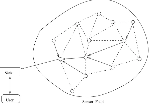
Sink
Sensor Field User
Fig. 2.1.Physical architecture of WSN.
protocols. For the performance evaluation, we considered two metrics: Routing Efficiency (RE) and goodput and we compare the simulation results for two cases: when the event node is mobile and stationary. The simulation results have shown that the routing efficiency for the case of mobile event node is better than the stationary event node using AODV protocol. Also, the goodput for the mobile event node case does not change too much compared with the stationary event case using AODV, but the goodput is not good when the number of nodes is increased.
The remainder of the paper is organized as follows. In Section 2, we explain the proposed network simulation model. In Section 3, we discuss the RE and goodput metrics. In Section 4, we show the simulation results. Conclusions of the paper are given in Section 5.
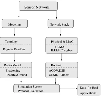
2. Proposed Network Simulation Model. In our WSNs, every node detects the physical phenomenon and sends back to the sink node data packets. In Fig. 2.1 is shown the physical architecture of WSN. We suppose that the sink node is more powerful than sensor nodes and it is always located a the borders of the service area. We analyze the performance of the network in a fixed time interval. This is the available time for the detection of the phenomenon and its value is application dependent. Proposed network simulation model is shown in Fig. 2.2.
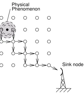
In this paper, we consider that a mobile event is moving randomly in the WSNs field. In Fig. 2.3 is shown one pattern of movement event’s path. We implemented a simulation system for WSNs considering moving event using ns-2. We evaluated the goodput and RE of AODV and DSR protocols using TwoRayGround propagation model and the lattice topology.
2.1. Topology. For the physical layout of the WSN, two types of deployment has been studied so far: the random and the lattice deployment. In the former, nodes are supposed to be uniformly distributed, while in the latter one nodes are vertexes of particular geometric shape, e.g. a square grid. as depicted in Fig. 2.4. In this work, we present results for the square grid topology only. In this case, in order to guarantee the connectedness of the network we should set the transmission range of every node to the step size, d, which is the minimum distance between two rows (or columns) of the grid. In fact, by this way the number of links that every node can establish (the node degree D) is 4. Nodes at the borders haveD= 2.
2.2. Radio Model. There are three basic models for the propagation of the radio signals of sensor nodes: Free space model, TwoRayGround model and Shadowing model. In a simple deterministic model, the received powerPrat a certain distancedis the same along all directions in the plane1. For example, in the case of Line
1
Sensor Network
Network Stack
Modeling
Topology
Physical & MAC
Regular Random
Radio Model
Shadowing
TwoRayGround
Routing
AODV,DSR
OLSR, Others
CSMA
IEEE802 Zigbee
Simulation System
Protocol Evaluation
Data for Real
Applications
Fig. 2.2.Network simulation model.
Of Sight (LOS) propagation of the signal, the Friis formula predicts the received power as:
Pr(d) =Pt−β (dB), (2.1)
β = 10 log
(4πd)2L GtGrλ2
whereGr andGtare the antenna gains of the receiver and the transmitter, respectively. λis the wavelength of the signal, Lthe insertion loss caused by feeding circuitry of the antenna, and β is the propagation pathloss. For omni-antennas,GR=Gt= 1. The signal decay is then proportional tod2.
In our simulation system, as a radio model we use TwoRayGround model. In this model the pathloss is:
β = 10 log
(4
πd)4L
GtGrhthrλ2
(2.2)
wherehrandhtare the receiver and transmitter antenna heights, respectively. The power decreases faster than Eq. (2.1) [6].
2.3. MAC protocol. We assume that the MAC protocol is the IEEE 802.11 standard. The receiver of every sensor node is supposed to receive correctly data bits if the received power exceeds the receiver threshold,γ. This threshold depends on the modulation scheme 2. As reference, we select parameters values according
to the features of a commercial device (MICA2 OEM). In particular, for this device, we found that for a central frequency of f = 916MHz and a data rate of 34KBaud, we have a threshold (or receiver sensitivity) γ=−98dBm [7]. The transmission range of sensor nodes should be at leastd. However, in the case of a general
2
Phenomenon
Physical
Fig. 2.3.One pattern of movement event path.
Sink node
Physical
Phenomenon
Fig. 2.4.Lattice topology.
Pt(d)|dB=
10βlog10
d d0
+γ−erfc−1(2p)p(2)σ
+ + 10 log10
d0
K 2
, (2.3)
where erfc−1is the inverse of the standard error function.
2.4. Routing Protocols. We are aware of many proposals of routing protocols for ad-hoc networks. Here, we consider reactive protocols such as AODV and DSR [8].
The AODV is an improvement of DSDV to on-demand scheme. It minimize the broadcast packet by cre-ating route only when needed. Every node in network should maintain route information table and participate in routing table exchange. When source node wants to send data to the destination node, it first initiates route discovery process. In this process, source node broadcasts Route Request (RREQ) packet to its neighbors. Neighbor nodes which receive RREQ forward the packet to its neighbor nodes. Neighbor nodes which receive RREQ forward the packet to its neighbors, and so on. This process continues until RREQ reach to the desti-nation node. When the intermediate nodes receive RREQ, they record in their tables the address of neighbors, thereby establishing a reverse path. When the node which knows the path to destination or destination node it-self receive RREQ, it sends back Route Reply (RREP) packet to source node. This RREP packet is transmitted by using reverse path. When the source node receives RREP packet, it can know the path to destination node and it stores the discovered path information in its route table. This is the end of route discovery process. Then, AODV performs route maintenance process. In route maintenance process, each node periodically transmits a Hello message to detect link breakage.
In DSR, the source node knows the entire path to the destination. And intermediate nodes don’t need to maintain route information table for neighbor’s address. This source routing information is stored in cache and updated when the node discover new route. DSR also consist of two mechanisms (Route Discovery and Route Maintenance processes). In route discovery process, DSR also uses RREQ and RREP as AODV. However in DSR, intermediate nodes don’t need to maintain route table because hop-by-hop path information (reverse path information) is stored in RREQ header when RREQ is forwarded from intermediate nodes. When destination node which knows the path to destination receives this RREQ packet, it sends back RREP to source node using header stored in RREQ packet. When the source node receives RREP packet, it knows the entire path to destination node and store the discovered path in cache. Route maintenance process is accomplished through the use of Route Error (RRER) packets. RRER packets are generated when the link is broken due to mobility of nodes.
2.5. Event Detection and Transport. As event detection and transport, we use the data-centric model similar to [9], where the end-to-end reliability is transformed into a bounded signal distortion concept. In this model, after sensing an event, every sensor node sends sensed data towards the MN. The transport used is a UDP-like transport, i. e. there is not any guarantee on the delivery of the data. While this approach reduces the complexity of the transport protocol and well fit the energy and computational constraints of sensor nodes, the event-reliability can be guaranteed to some extent because of the spatial redundancy. The sensor node transmits data packets reporting the details of the detected event at a certain transmission rate3. The setting
of this parameter,Tr, depends on several factors, as the quantization step of sensors, the type of phenomenon, and the desired level of distortion perceived at the MN. In paper [9], the authors used this Tr as a control parameter of the overall system. For example, if we refer to event-reliability as the minimum number of packets required at MN in order to reliably detect the event, then whenever the MN receives a number of packets less than the event-reliability, it can instruct sensor nodes to use a higherTr. This instruction is piggy-backed in dedicated packets from the MN. This system can be considered as a control system, as shown in Fig. 2.5, with the target event-reliability as input variable and the actual event-reliability as output parameter. The target event-reliability is transformed into an initial Tr0. The control loop has the output event-reliability as input, and on the basis of a particular non-linear functionf(·),Tr is accordingly changed. We do not implement the entire control system, but only a simplified version of it. For instance, we varyTr and observe the behavior of the system in terms of the mean number of received packets. In other words, we open the control loop and analyze the forward chain only.
3
T
r0f()
T
r WSNTarget event−reliability
Event−reliability
Fig. 2.5.Representation of the transport based on the event-reliability.
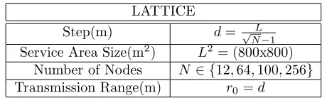
Table 4.1
Topology settings.
LATTICE
Step(m) d= L
√
N−1
Service Area Size(m2) L2= (800x800)
Number of Nodes N ∈ {12,64,100,256}
Transmission Range(m) r0=d
3. Goodput and Routing Efficiency. In this section, we introduce the performance evaluation metrics: goodput and RE. We consider that after a sensor node detects the physical phenomenon, it sends the packets to the sink node via a routing protocol. The ability for transmitting packets for different protocols is different. Also, the RE of a protocol is affected by many network parameters such as wireless transmission radio model, network topology, and transmission frequency [4]. In order to compare the performance of different protocols, we consider the same simulation environment. For our system, we used TwoRayGround radio model and the network topology is regular [10, 11].
The goodput is defined at the sink, and it is the received packet rate divided by the sent packets rate. Thus:
G(τ) = Nr(τ) Ns(τ)
(3.1)
whereNr(τ) is the number of received packet at the sink, and theNs(τ) is the number of packets sent by sensor nodes which detected the phenomenon. Note that the event-reliability is defined asGR= N
r(τ)
R(τ), whereRis the
required number of packets or data in a time interval ofτ seconds.
We defined the RE parameter as the ratio of sent packets from sensing node with sent packet by routing protocol. Thus:
RE(τ) = Nsent(τ) Nrouting(τ)
(3.2)
whereNrouting(τ) is the number of sent packets by routing protocol, andNsent(τ) is the number of sent packets by sensor nodes which detect the phenomenon.
4. Simulation Results. In this section, we present the simulation results. We implemented the simulation system using ns-2 simulator, with the support of NRL libraries [12]. For each routing protocol, the sample results of Eq. (3.1) and Eq. (3.2) are computed over 20ssimulation runs.
The settings of our lattice are shown in Table 4.1. The sensing range is assumed to be half of the transmission range. The radio model parameters are listed in Table 4.2.
Radio model and system parameters.
RADIO MODEL PARAMETERS Path Loss Coefficient α= 2.7
Variance σ2dB= 16dB
Carrier Frequency 916MHz
Antenna Omni
Threshold (sensitivity) γ=−118dB OTHER PARAMETERS
Reporting Frequency Tr= [0.1,1000]pps1 Interface Queue Size 50 packets
UDP Packet Size 100 bytes
Detection Intervalτ 30s
1packet per seconds
10−1 100 101 102 103
10−3 10−2 10−1 100 101 102 103
T r(pps)
R
E
Routing Efficiency (AODV ,TwoRayGround)
N=12
N=64
N=100
N=256
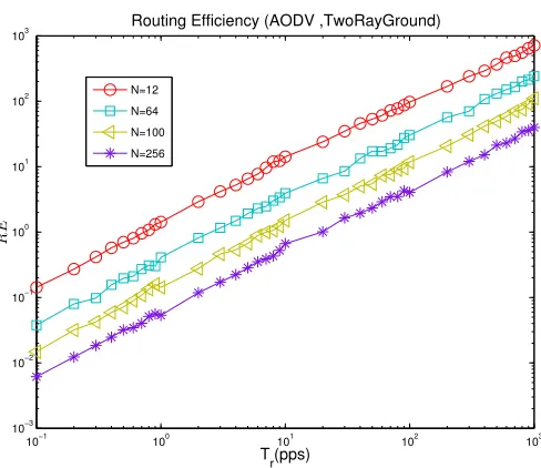
Fig. 4.1.RE for stationary event (AODV).
node is higher than the number of packets used by routing protocol. In case of AODV, the RE decreases with the increase of number of sensor nodes. It should be noted that when the number of sensor nodes is increased, the number of routes is increased, thus the searching time to find a route also is increased. When the number of nodes is 256, the RE of AODV is the worst in our simulation. The simulation results for the case of mobile event are shown in Fig. 4.2. The RE is stable and better than in case of stationary event, especially when the number of nodes is increased. WhenN = 12, the performance is almost the same for both cases. But, in the cases ofN = 64, N= 100, N= 256, the performance is better for mobile event case.
10−1 100 101 102 103 10−2
10−1 100 101 102 103
T r(pps)
R
E
Routing Efficiency(AODV,TwoRayGround,Mobile)
N=12
N=64
N=100
N=256
Fig. 4.2. RE for mobile event (AODV).
10−1 100 101 102 103
10−2 10−1 100 101 102 103 104
T r(pps)
R
E
Routing Efficiency (DSR ,TwoRayGround)
N=12
N=64
N=100
N=256
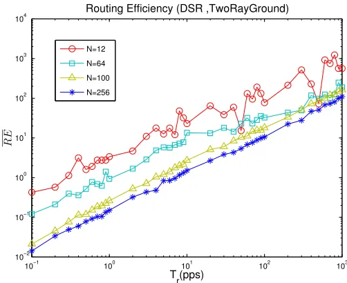
Fig. 4.3.RE for stationary event (DSR).
number of nodes is increased, the goodput is increased. However, the goodput of stationary event is better than mobile event, but the goodput of mobile event is more stable.
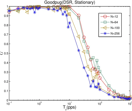
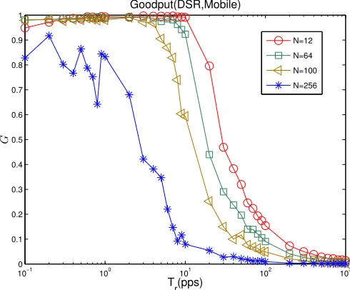
In case of DSR, as shown in the Fig. 4.7, the goodput of stationary event is almost the same with AODV (see Fig. 4.5). However, in case of mobile event (see Fig. 4.8), with the increase of number of nodes, the value of goodput is decreased much more compared with stationary event case. When the number of nodes is 256 the goodput is the worst and is not stable.
10−1 100 101 102 103 10−1
100 101 102 103
T r(pps)
R
E
Routing Efficiency(DSR,TwoRayGround,Mobile)
N=12
N=64
N=100
N=256
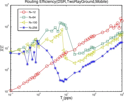
Fig. 4.4.RE for mobile event (DSR).
10−1 100 101 102 103
0 0.1 0.2 0.3 0.4 0.5 0.6 0.7 0.8 0.9 1
Tr(pps)
G
Goodput( AODV ,TwoRayGround)
N=12
N=64
N=100
N=256
Fig. 4.5.Goodput for stationary event (AODV).
5. Conclusions. In this paper, we presented the implementation of a simulation system for WSNs using ns-2. We considered for simulations AODV and DSR protocols and evaluated the proposed system for two cases: stationary event and mobile event. For evaluation, we considered goodput and RE metrics.
From the simulation results, we conclude as follows.
• In case of AODV, the RE decreases with the increase of number of sensor nodes. When the number of nodes is 256, the RE of AODV is the worst.
• In the case of mobile event, for AODV protocol, the RE is stable and better than in case of stationary event, especially when the number of nodes is increased.
• Comparing with AODV for the same time interval and the number of nodes, the RE of DSR is better than AODV, but it is unstable.
10−1 100 101 102 103 0
0.1 0.2 0.3 0.4 0.5 0.6 0.7 0.8 0.9 1
Tr(pps)
G
Goodput(AODV, Mobile)
N=12
N=64
N=100
N=256
Fig. 4.6.Goodput for mobile event (AODV).
10−1 100 101 102 103
0 0.1 0.2 0.3 0.4 0.5 0.6 0.7 0.8 0.9 1
Tr(pps)
G
Goodpug(DSR, Stationary)
N=12
N=64
N=100
N=256
Fig. 4.7.Goodput for stationary event (DSR).
• In case of DSR, the goodput of stationary event is almost the same with AODV. However, in case of mobile event with the increase of number of nodes, the value of goodput is decreased much more compared with stationary event case. When the number of nodes is 256, the goodput is the worst and is not stable.
• The goodput of AODV is better than DSR in case of mobile event.
In the future, we would like to carry out more extensive simulations for many mobile events and other protocols. We also would like to consider the case of Shadowing radio model and the random topology.
10−1 100 101 102 103 0
0.1 0.2 0.3 0.4 0.5 0.6 0.7 0.8 0.9 1
T r(pps)
G
Goodput(DSR,Mobile)
N=12
N=64
N=100
N=256
Fig. 4.8.Goodput for mobile event (DSR).
REFERENCES
[1] S. Giordano and C. Rosenberg,“Topics in Ad Hoc and Sensor Networks”, IEEE Communication Magazine, Vol. 44, No.
4, pp. 97–97, 2006.
[2] J. N. Al-Karaki and A. E. Kamal,“Routing Techniques in Wireless Sensor Networks: A Survey”, IEEE Wireless
Commu-nication, Vol. 11, No. 6, pp. 6–28, December 2004.
[3] G. W.-Allen, K. Lorincz, O. Marcillo, J. Johnson, M. Ruiz, J. Lees, “Deploying a Wireless Sensor Network on an
Active Volcano”, IEEE Internet Computing, Vol. 10, No. 2, pp. 18–25, March, 2006.
[4] O. Younis, S. Fahmy,“HEED: A Hybrid, Energy-efficient, Distributed Clustering Approach for Ad-hoc Sensor Networks”,
IEEE Transactions on Mobile Computing, Vol. 3, No. 4, pp. 366–379, 2004.
[5] T. Yang, G. De Marco, M. Ikeda, L. Barolli,”A Case Study of Event Detection in Lattice Wireless Sensor Network with
Shadowing-Induced Radio Irregularities”, Proc. of MoMM-2006, Yogyakarta, Indonesia, pp. 241–250, December 2006.
[6] T. S. Rappaport, “Wireless Communications”,Prentice Hall PTR, 2001.
[7] Crossbow Technology, Inc.,htpp://www.xbow.com/
[8] C. Perkins,“Ad Hoc Networksc”, Addison-Wesley, 2001.
[9] Ozg¨¨ ur B. Akan and I. F. Akyildiz,“Event-to-Sink Reliable Transport in Wireless Sensor Networks”, IEEE/ACM
Trans-actions on Networking, Vol. 13, No. 5, pp. 1003–1016, 2005.
[10] W. Ye, J. Heidemann, D. Estrin,“Medium Access Control with Coordinated Adaptive Sleeping for Wireless Sensor
Net-works”, IEEE/ACM Transaction Networking, Vol. 12, No. 3, pp. 493–506, 2004.
[11] G. Zhou, T. He, S. Krishnamurthy, J. A. Stankovic, “Models and Solutions for Radio Irregularity in Wireless Sensor
Networks”, ACM Transaction on Sensors Network, Vol. 2, No. 2, pp. 221–262, 2006.
[12] I. Donward, “NRL’s Sensor Network Extension to NS-2”,http://pf.itd.nrl.navy.mil/nrlsensorsim/2004.
[13] V. C. Gungor, M. C. Vuran, O. B. Akan,“On the Cross-layer Interactions Between Congestion and Contention in Wireless
Sensor and Actor Networks”, Ad Hoc Networks Journal (Elsevier), Vol. 5, No. 6, pp. 897–909, August 2007.
[14] M. Zuniga and B. Krishnamachari,“An Analysis of Unreliability and Asymmetry in Low-power Wireless Links”, http:
//www-scf.usc.edu/marcozun/ 2006.
Edited by: Fatos Xhafa, Leonard Barolli
Received: September 30, 2008