Organized by C.O.E.T, Akola, ISTE, New Delhi & IWWA. Available Online at www.ijpret.com59
INTERNATIONAL JOURNAL OF PURE AND
APPLIED RESEARCH IN ENGINEERING AND
TECHNOLOGY
A PATH FOR HORIZING YOUR INNOVATIVE WORK
EVALUATION OF EIGEN VALUES AND EIGEN VECTORS FOR FREE VIBRATION
ANALYSIS USING FINITE ELEMENT PROCEDURES
R R GADPAL
Department of Applied Mechanics, Govt. Polytechnic, Arvi , Dist.(Wardha)
Accepted Date: 07/09/2016; Published Date: 24/09/2016
Abstract:The generalised problem in free vibration analysis of any structure is that of evaluating an eigenvalue λ (= ω2), which is a
measure of the frequency of vibration together with the corresponding eigenvector x indicating the mode shape. This presentation consists of determination of fundamental vibration frequencies of a general structure. The frequencies can be determined by the finite element method using characteristic polynomial technique, Vector iteration technique and transformation methods.. Power iteration, inverse iteration and subspace iteration methods use the property of the Rayleigh quotient. Power iteration leads to evaluation of the largest eigenvalue. Subspace iteration technique is suitable for large scale problems and used in several codes. The inverse iteration scheme can be used for evaluating the lowest eigenvalues. The basic approach in transformation method is to transform the matrices to a simpler form and then to determine the eigenvalues and eigenvectors. In this presentation the main focus is to discuss the transformation method, to develop the related computer program and validate the results. The results show good agreement with those determined by classical method.
Keywords: Free vibration analysis, Fundamental natural frequencies, Mode shapes, Eigenvalues and Eigenvectors , Generalised eigenproblem, Standard eigenproblem, Stiffness and mass matrices.
.
Corresponding Author: MR. R R GADPAL
Co Author: Access Online On:
www.ijpret.com
How to Cite This Article:
R. R. Gadpal, IJPRET, 2016; Volume 5 (2): 59-69 PAPER-QR CODE
SPECIAL ISSUE FOR
INTERNATIONAL CONFERENCE ON
Organized by C.O.E.T, Akola, ISTE, New Delhi & IWWA. Available Online at www.ijpret.com60
INTRODUCTION
Free vibration analysis is often required for most of the important structures / structural elements in the field of civil, mechanical, automobile, aerospace, optical, marine, nuclear and structural engineering. The differential characteristics in free vibration analysis enable engineers to design better and lighter structures. The Study of their free vibration behaviour is very important to the structural engineers when these structures are subjected to external complicated dynamic loads such as earthquake, wind, impact and wave forces. An understanding of the free vibration frequencies of any system (especially, the fundamental frequency) is the prerequisite to the understanding of its response to forced vibration. In civil engineering, buildings, horizontal floors, beams, columns are directly exposed to static and dynamic loadings. To determine the eigenvalues and eigenvectors which are the measure of the frequency of vibration and mode shapes the suitable method is to be selected by the analyst as per the requirements in design of structures.
II LITERATURE REVIEW
The literature of eigenproblems is quite large, both for theoretical aspects and numerical algorithms, and only a small fraction of it can be cited. Hughes T.J.R. [1], Bathe K. J. [2] and Kardestuncer H. [3] have written extensive discussions about eigenproblems in their Finite Element Books. Wilkinson J.H. [4] wrote a book about the algebraic eigenvalue problem in 1965. Bathe K. J. and Wilson E.L. [5] published a paper on solution methods for eigenvalue problems in structural mechanics in 1973. In 1980, Parlett B.N. [6] introduced the method for solution of the symmetric eigenvalue problem. In 1984, Jennings A. [7] wrote about eigenvalue methods for vibration analysis. Sehmi N.S. [8] gave large order structural eigenvalue techniques in 1989. Cheung Y.K. and Leung A.Y.T. [9]. published a book on finite element methods in dynamics in 1991 In 1994, Tichler V.A. and Venk ayya V.B. [10] evaluated eigenvalue routines for large scale applications. Bertolini A.F. [11] reviewed eigensolution procedures for linear dynamic finite element analysis in 1998.
Undamped free vibration analysis of the entire building is performed as per established methods of mechanics using appropriate masses and elastic stiffness of the structural system to obtain natural period (T) and mode shape {ɸ} of those of its modes of vibration that need to be considered as per I.S.1893-2002(part 1) clause No. 7.8.4.2.[12]
Organized by C.O.E.T, Akola, ISTE, New Delhi & IWWA. Available Online at www.ijpret.com61 Thus the present study evaluates the first few dominant modes of vibration frequencies of structures. The frequencies estimated by the proposed formulation and program coincide well with those obtained by the finite element method, which can serve as a design aid for structural engineers.
III. FINITE ELEMENT FORMULATION
For a positive definite symmetric stiffness matrix [K] of size n x n, there are n real eigenvalues and corresponding eigenvectors satisfying equation (1).
[K] – λ [M] {x} ={0} ...(1)
The above eigenproblem asks for the values of a scalar λ such that the matrix equation (1) has solutions other than trivial solution {x} = {0}. There are at most n nonzero roots λi , not
necessarily all distinct. The λi are called eigenvalues, characteristic values, latent roots or principal values. The eigenvalues may be arranged in ascending order such that
0 ≤ λ1 ≤ λ2 ≤ ... ≤ λn ... (2) The vector corresponding to each λi is an {x}i called as an eigenvector, characteristic vector, principal vector, normal mode or natural mode. The eigenvectors possess the property of being orthogonal with respect to both the stiffness and mass matrices:
xiT M xj = 0 if i ≠ j
xiT K xj = 0 if i ≠ j ...(3)
The lengths of eigenvectors are generally normalized so that
xiT M xj = 1 ... (4)
The foregoing normalization of the eigenvectors leads to the relation
xiT K xj = λi ... (5)
In many codes, other normalization schemes are also used. The length of an eigenvector may be fixed by setting its largest component to a preset value, say, unity.
The eqn (1) in the form ([K] – λ [M]){x} ={0} is called generalised eigenproblem or simply eigenproblem and further can be simplified as
[K] {x} = λ [M] {x} ...(6)
If , however, matrix [M] happens to be identity matrix [ I ] or premultiplying both sides of above equation by [M -1] , we get,
[M -1] [K] {x} = λ [M -1] [M]) {x}
[A] {x} = λ [ I ] {x}
or [A] {x} = λ{x} ...(7) where, [A] = [M -1] [K]
Organized by C.O.E.T, Akola, ISTE, New Delhi & IWWA. Available Online at www.ijpret.com62 If {x} contain only d.o.f. that may assume non-zero values after all rigid-body modes and mechanisms (if any) are suppressed, thus [K] is positive definite. If element mass matrices are consistent or lumped with strictly positive definite, [M] is also positive definite. Then the number of non-zero λi is equal to number of d.o.f. in {x}. Occasionally two or more λi are numerically equal. Then there associated vibration modes {x}i are not unique, but mutually orthogonal modes for the repeated λi can be established. A partly or completely unconstrained structure or a structure that contains a mechanism, has a positive semidefinite [K] and a zero eigenvalue associated with each possible rigid body motion or mechanism . The associated mode shape describes the rigid body motion or the mechanism motion. If [M] is lumped with some zero diagonal coefficients, an infinite eigenvalue is associated with each Mii. Degrees of freedom associated with Mii can be removed by static condensation [13] before extracting eigenvalues, without affecting the remaining eigenvalues and mode shapes.
The eigenvalue and eigenvector evaluation procedures fall into the following basic categories. 1. Characteristic polynomial technique
2. Vector iteration techniques 3. Transformation methods
Amongst these methods, transformation methods are suitable for large scale problems and will be discussed in details.
Characteristic Polynomial
From eqn.(6), we have ([K] – λ [M]){x} ={0}. If the eigenvector is to be non-trivial, the required condition is
det ([K] – λ [M]) ={0} ... (8)
This represents the characteristic polynomial in λ.
The characteristic polynomial method can solve 2 x 2 problems by hand calculations. However it is also found uneconomical for computer usage because it is rather tedious and requires further mathematical considerations. We now discuss the other two categories.
Vector Iteration Methods
Various vector iteration methods use the properties of Rayleigh Quotient. For the generalised eigenvalue problem given in eqn. (6), Rayleigh quotient can be defined as ,
Q (v) = ...
(9)
Organized by C.O.E.T, Akola, ISTE, New Delhi & IWWA. Available Online at www.ijpret.com63
λ1 ≤ Q (v) ≤ λn ... (10)
In the inverse iteration scheme [14], we start with a trial vector xo and obtain the eigenvector xk after normalization and satisfying the requirements of tolerance. This scheme converges to the lowest eigenvalue, provided the trial vector does not coincide with the one of the eigenvectors. Other eigenvalues can be obtained by shifting, or by taking the trial vector from a space that is M – orthogonal to the calculated eigenvectors.
Transformation Methods
The basic approach in this method is to transform the matrices to a simpler form and then to determine the eigenvalues and eigenvectors. The major methods in this category are the generalised Jacobi Method and the QR method. These methods are suitable for large-scale problems. In the QR method, the matrices are firs reduced to tridigonaliztion form using Householder matrices. The generalised Jacobi Method uses the transformation to simultaneously diagonalize the stiffness and mass matrices. This method needs the full matrix locations and is quite efficient for calculating all eigenvalues and eigenvectors for small problems.
If all the eigenvectors are arranged as columns of a square matrix X and all eigenvalues as the diagonal elements of a square matrix Ʌ, then the generalised eigenvalue problem can be written in the form
[K] [X ] = [M] [ X ] [Ʌ] ... (11)
where , [ X ] = [ X1, X2 ,..., Xn ] ... (12)
[Ʌ] = ...
(13)
Using M- orthonormality of eigenvectors, we have,
[X]T [ M ] [ X ] = [Ʌ] ... (14)
and
[X]T [ K ] [ X ] = [ I ] ... (15)
where [ I ] = Identity matrix
Generalised Jacobi Method
In the generalised Jacobi method a series of transformations P1, P2,..., Pl are used such that if
P represents the product
Organized by C.O.E.T, Akola, ISTE, New Delhi & IWWA. Available Online at www.ijpret.com64 Then the off diagonal terms of PTKP and PTMP are zero. In practice, the off-diagonal terms are
set to be less than a value smaller than tolerance.
[ K*] = [P
l ]T .... [P2]T[P1]T[ K] [ P1] [ P2] .... [ Pl ] ... (17a)
[ M*] = [P
l ]T .... [P2]T[P1]T[ M] [ P1] [ P2] .... [ Pl ] ... (17b)
[ K*] and [ M*] are the diagonal matrices. To eliminate [ K
ij] and [ Mij] simultaneously we have
to let transformation matrix [ P ] in such a way that at step k,
[ Pk ] = and thus, [ Pk ]T = .... (18)
[ Pk ] has all diagonal elements equal to 1, has a value of α at row i and column j and β at row j
and column i , and all other elements equal to zero. The scalars α and β are chosen so that the ij locations of PkTKP and PkTMP are simultaneously zero.
PkTKP =
Considering only 2 and 4 rows and 2 and 4 columns are affected
Thus new K24 = = (1+ )
Now in general in order to make the non-diagonal elements equal to zero we can write PkTKP
Organized by C.O.E.T, Akola, ISTE, New Delhi & IWWA. Available Online at www.ijpret.com65
(1+ ) = 0 ... (19)
and (1+ ) = 0 ... (20)
Premultiplying eqn (19) by and eq. (20) by and solving the simultaneous equations, we get
α ( - + β ( - = 0
or α ( + β ( = 0 ... (21)
where, A = ( - and B = ( -
Solving Eqn (21) , β = - and after substituting in eqn (19), we get
- = 0 ... (22)
Multiplying eqn (22) by B and dividing by we get
B - A + - = 0
A + α - B = 0 ... (23)
Introducing C = and substituting values of A and B, we get
C =
Multiplying eqn (23) by 0.5, we get
0.5 A + 0.5 α C - 0.5 B = 0 ... (24)
Solving eqn (24) , we get
α = ... (25)
Particularly,
When, A ≠ 0, B ≠ 0, α = and β = - ;
A = 0, β = 0 and α = - ;
Organized by C.O.E.T, Akola, ISTE, New Delhi & IWWA. Available Online at www.ijpret.com66 When both A and B are zero, any one of the two values listed can be chosen.
Adopting the above procedure for determination of matrices [ K*] and [ M*] in eqs. (17), the
eigenvalues and eigenvectors are given by,
λii = and xij = , or in general
Ʌ = and X = ... (27)
where, = and = ... (28) In the generalized Jacobi program, the elements of K and M are zeroed out in the order indicated in fig.1. Once Pk is defined by determining α and β, PkT[ ]Pk can be performed on K
and M as shown in fig.2. Also by starting with P = I, the product PPk is computed after each
step. When all elements are covered as shown in fig.1, one pass is completed . After operations at step k, some of the previously zeroed elements are altered. Another pass is conducted to check for the value of the diagonal elements. The transformation is performed if the elements
at ij is larger than a tolerance value. A tolerance 10-6 smallest Kii is used for stiffness, and
10-6 largest Mii is used for the mass. The tolerance can be redefined for higher accuracy. The process stops when all off-diagonal elements are less than the tolerance.
Organized by C.O.E.T, Akola, ISTE, New Delhi & IWWA. Available Online at www.ijpret.com67 If the diagonal masses are less than the tolerance, the diagonal value is replaced by the tolerance value, thus, a large eigenvalue will be obtained. In this method K need not be positive definite. On the basis of above formulation a computer program is developed and results are compared with the standard available results.
IV NUMERICAL EXAMPLE
Example 1: A cantilever having geometrical and material properties is as shown in fig. 3
Determine all the eigenvalues and eigenvectors for the beam shown in fig. 3 using the program developed on the basis of above formulation.
(a)
E = 200 GPa, ρ = 7840 kg/m3, I = 2000 mm4, A = 240 mm2
(b)
Fig. 3 Cantilever Beam Model Solution :
Organized by C.O.E.T, Akola, ISTE, New Delhi & IWWA. Available Online at www.ijpret.com68
K = ; M = 0.001
The input data for the developed program is same as that for inverse iteration program. However, the program coverts to full matrices in calculations. Convergence occurs at the fourth sweep. The solution is presented in Table1. and compared with the standard results.
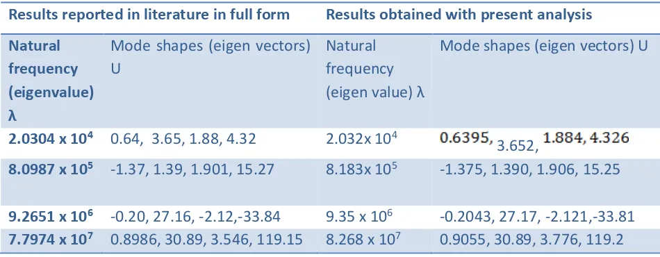
Table 1. Natural frequencies & Mode shapes
Results reported in literature in full form Results obtained with present analysis
Natural frequency (eigenvalue) λ
Mode shapes (eigen vectors) U
Natural frequency (eigen value) λ
Mode shapes (eigen vectors) U
2.0304 x 10⁴ 0.64, 3.65, 1.88, 4.32 2.032x 10⁴
3.652,
8.0987 x 10⁵ -1.37, 1.39, 1.901, 15.27 8.183x 10⁵ -1.375, 1.390, 1.906, 15.25
9.2651 x 10⁶ -0.20, 27.16, -2.12,-33.84 9.35 x 10⁶ -0.2043, 27.17, -2.121,-33.81
7.7974 x 10⁷ 0.8986, 30.89, 3.546, 119.15 8.268 x 10⁷ 0.9055, 30.89, 3.776, 119.2
The natural fundamental frequencies of the structure / component can be determined using classical methods as well as using finite element technique which is widely reported in the literature. It is well known that the numerical analysis results are valid only for particular values of the parameters considered in the analysis. The structural engineers concerned with dynamic analysis or design of structures need a design formula or program for rapid determination of the governing natural frequency. The numerical values obtained by running the program are quite gratifying with those reported in literature[16] and reproduced in Table 1.
VI CONCLUSIONS:
The fundamental frequencies and mode shapes were determined by finite element method. The devised program is quite useful for determining Fundamental natural frequencies, Mode shapes, by evaluating eigenvalues and eigenvectors in the Generalised eigenproblem.,
REFERENCES:
Organized by C.O.E.T, Akola, ISTE, New Delhi & IWWA. Available Online at www.ijpret.com69 2. Klaus.-.Jurgen Bathe - Finite Element Procedures , Fourth Reprint, Prentice Hall of India Pvt. Ltd. (1997).
3. Kardestuncer H.,ed, Finite Element Handbook, McGraw Hill, New York, (1987).
4. Wilkinson J.H., The Algebraic Eigenvalue Problem, Clarendon Press, Oxford, U.K., (1965) 5. Bathe K. J. and Wilson E.L. “Solution Methods for Eigenvalue Problem in Structural Mechanics”, International Journal for Numerical Methods in Engineering, Vol.6, No. 2, pp 213-226 (1973).
6. Parlett B.N.- “The symmetric Eigenvalue Problem”’ Prentice Hall of India Pvt. Ltd, Englewood Cliffs, NJ, (1980).
7. Jennings A.– “Eigenvalue Methods for Vibration Analysis”, Shock and Vibration Digest, Vol. 16, No.1 , pp 25 -33, (1984).
8. Sehmi N.S., - “Large order Structural Eigen Analysis Techniques, Ellis Horwood Ltd., Chichester, U.K. (1989).
9. Cheung Y.K. and Leung A.Y.T.,-“Finite Elemnt Methods in Dynamics, Kluwer Academic Publishers, Dordrecht (1991).
10. Tichler V.A. and Venk ayya V.B.,- “Evaluation of eigenvalue Routines for Large Scale Applications, Shock and Vibration, Vol. 1, No.3 , pp 201 -216 (1994).
11. Bertolini A.F.,- “Review of Eigensolution Procedures for Linear Dynamic Finite Element Analysis, ASME Applied Mechanics Reviews, Vol. 51, No. 2, pp 155-172, (1998).
12. IS 1893:2002 – Criteria for Earthquake Resistant Design of Structures (Part 1), pp 24-26, (2002).
13. Gadpal R.R.,- “Reduction Techniques in Dynamic Analysis of Structures”, International Journal of Pure and Applied Research in Engineering and Technology, Vol. 4 (9), pp 143-152, (2016)
14. Gadpal R.R.,- “Dynamic Analysis of Structures under Free Vibrations using Finite Element and Inverse Iteration Technique”, International Journal of Modern Trends in Engineering and Research, Vol. 2, Issue (2), pp 113-118, (2015)
15. Meghre A.S. and Kadam K.N.,- “ Finite Element Method in Structural Analysis”, Khanna Publishers, First Edition, (2014).