Spatio-temporal variation analysis of soil temperature based on wireless sensor network

Spatio-temporal variation analysis of soil temperature based on

wireless sensor network

Liu Hui

,

Meng Zhijun

,

Wang Hua

,

Xu Min

2. National Engineering Research Center for Information Technology in Agriculture, Beijing 100097, China)

Abstract: Soil temperature is a key factor for best planting dates decision-making in the large scale farming areas of northeast China because of high latitudes and frigid environment. Continuous data were collected from a wireless sensor network (WSN)-based monitoring system to exactly analyze and understand soil temperature of the whole farmland. Using the classical statistics and geo-statistics methods, real-time monitoring data were analyzed with three aspects, i.e. temporal variation, spatial variation and spatio-temporal variation. Temporal variation analysis of each sensor node showed a sinusoidal curve of daily soil temperature and gave the long-term trend of daily average soil temperature in a certain period. Spatial variation analysis provided the spatial distribution map of daily average soil temperature within a study region for a certain day. Spatio-temporal variation analysis quantified the variation process of the spatial distribution over time by the monitored classes distribution indicator (MCDI) proposed. Experimental results showed that the above variations analysis of the real-time data provide an effective approach to determine whole-farmland soil temperature.

Keywords: precision agriculture, soil temperature dynamics, spatial-temporal variability, spatial variation, wireless sensor network (WSN)

DOI: 10.3965/j.ijabe.20160906.1871

Citation: Liu H, Meng Z J, Wang H, Xu M. Spatio-temporal variation analysis of soil temperature based on wireless sensor network. Int J Agric & Biol Eng, 2016; 9(6): 131－138.

1 Introduction

Soil temperature is a major driver of the vegetation growth and soil biological activity[1], therefore it is a key factor for best planting dates decision-making in the large scale farming areas of northeast China, where the soil temperature is a restrictive requirement for planting because of high latitudes and frigid environment. In practice, soil temperature of a random sample obtained from the farm field is measured as an important indicator.

Received date: 2015-04-19 Accepted date: 2016-10-08

Biography: Liu Hui,PhD, Associate Professor, research interests: ICT application in precision agriculture, Email: liuhui_mail@ 163.com; Wang Hua,PhD, Associate Professor, research interests: data mining, Email: [email protected]; Xu Min, PhD, Lecturer, research interests:computer vision,Email: [email protected]. *Corresponding author:Meng Zhijun, PhD, Professor, research interests: intelligent agricultural equipment. Mailing address: Room A-517, Beijing Nongke Mansion, No.11 Shuguang Huayuan Middle Road, Beijing 100097, China. Tel: +86-10-51503785, Email: [email protected].

But this method is not rigorous in science. As a matter of fact, spatial and temporal variation of soil properties

has been scientifically acknowledged[2,3]. Therefore,

multiple locations are usually required for sampling so as to exactly analyze and understand the spatio-temporal variation during the field survey in precision agriculture (PA). However, it is arduous to collect data frequently with a very high spatial sampling density.

As a popular technology, wireless sensor network (WSN) is quite suitable for the PA real-time monitoring[4]. The WSN is characterized by the dense deployment of sensor nodes which monitor the physical phenomenon continuously. Many PA monitoring applications were established as well as research projects. Zhang et al.[5]

established a wireless sensor network system including twenty sensor nodes, two sink nodes, and a high resolution web-camera for monitoring soil moisture.

Dong et al.[6] designed autonomous irrigation

system by monitoring the soil conditions in real time using a wireless underground sensor network. Li et al.[7] developed and deployed a soil property monitoring system in a wheat field, and evaluated the quality of service of the system. A wireless sensor network composed of 135 soil moisture sensors and 27 temperature sensors was reported for monitoring soil moisture dynamics in an apple tree orchard[8].

The WSN technology makes it possible to acquire dynamic data of soil property to achieve real-time spatio-temporal statistics and operation. In the continuous sampling networks, the reading of any sensor node is a single sample representing the value of a location at some time. The true value of the monitoring network is to obtain continuous spatio-temporal variation of a certain physical variable by interpolating the values of the field where there is no sensor sampling. A theoretical framework for modeling the spatial and

temporal correlations in WSN was discussed[9].

Heathman et al.[10] proposed that the adequacy of

long-term point-scale measurements of surface soil moisture could represent the local-field-scale averages, serving as the calibration and validation of remotely sensed soil moisture. Additionally, a map of soil moisture distribution was obtained using the Kriging interpolation method combined with a WSN-based monitoring system[11]. However, little information has been mentioned with respect to specific spatio-temporal variation methods for processing massive actual data. This research aimed to study how to analyze continuous

sampling data obtained from the WSN applications in order to satisfy the requirements such as whole-farmland soil temperature determination for best planting dates decision-making.

2 Materials and methods

2.1 Architecture of soil temperature monitoring system

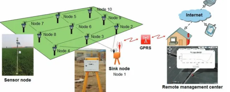
At the National Experimental Farm of Precision Agriculture, Beijing, China, a wireless sensor network was deployed for monitoring soil temperature in a wheat field in the summer of 2013. The network consisted of nine sensor nodes, a sink node and a remote management center (Figure 1). The sensor nodes were installed in a sampling grid pattern with a 60 m interval to satisfy the requirements of communication range and sampling range for WSNs[12]. Each sensor node was connected to a sensor for measuring soil temperature. The sink node was designed to collect data from all the sensor nodes. Consequently, the collected data were transformed to the remote management center through integrated GPRS module. The application server software running in the remote management center performed the functions of data display, storage, analysis and release. Users accessed and downloaded the monitored data with terminal computers or mobiles via the internet. Besides that, a weather station was installed in the same field to obtain the meteorological data including air temperature, relative humidity, precipitation, solar radiation and so on.

Figure 1 System architecture of the wireless sensor network for monitoring soil temperature

In this experiment, soil temperature was measured by the CG-3 sensor (Handan Qingsheng Electronics

November, 2016 Liu H, et al. Spatio-temporal variation analysis of soil temperature based on WSN Vol. 9 No.6 133

measurement, the sensor probe was placed horizontally in the soil, and the measurement accuracy was ±0.2°C. Since most of the soil ecosystem processes occurred within the top layers of soil, each soil temperature sensor was buried about 10 cm underground. This depth could better guarantee high stability and reliability of data acquisition over a long period in the rainy season. Soil temperature data of each sensor node was sampled once every 10 min.

2.2 Data analysis

2.2.1 Temporal variation analysis of each sensor node Soil temperature fluctuates daily due to variations of air temperature and solar radiation. Although the soil temperature changes more slowly than the air temperature, it still has a large temperature variation during single day. It is found that the soil temperature varied similarly each day[13]. The maximum and minimum values of the soil temperature appeared at similar times. A series of non-linear regressions was computed based on the daily soil temperature collected from different sensor nodes during the experiment. In this study, a sinusoidal non-linear model was proposed and utilized for data analysis. The applied model for measuring soil temperature at a certain depth is expressed as following:

( ) sin(2π / 1440)

T t = + ⋅T A ⋅t (1)

where, T(t) is the soil temperature at time t (min) in

1440 min a day, °C; T denotes the daily average soil

temperature, °C. As a parameter characterizing the

annual variation of soil temperature around the average value, is the fluctuation amplitude of daily soil temperature, which is calculated by:

max min

( ) / 2

A= T −T (2)

where, Tmax is the maximum soil temperature in a day, °C;

Tmin is the minimum of soil temperature, °C.

In the model, T

,

following statistical equations respectively:

1 1 ( ) n i i

T T t

n =

=

∑

max [ ( )]i

T =Max T t

min [ ( )]i

T =Min T t (5) where, T(ti) is the i-th observation of soil temperature

during a day among the total observations, °C.

Comparing with the daily soil temperature, more attention was paid on the long-term trends of soil temperature in a certain period. Daily average soil temperature is usually used to indicate the soil temperature condition at the sampling location in a day. Therefore, the daily average soil temperature data were calculated and demonstrated with time series of about 30 d in this study.

2.2.2 Spatial variation analysis for a certain day

As is known, most soil properties vary continuously in space. Spatial variation of soil properties was generally analyzed with the geo-statistics method. The goal of the geo-statistical analysis is to generate a spatial distribution map by interpolating the values of unobserved locations based on the neighboring measurements. As an advanced geo-statistical interpolation, kriging was described in many published books and papers. Kriging interpolation mainly includes simple kriging, ordinary kriging, universal kriging,

co-kriging and others[14]. The most robust and

commonly used method is the ordinary kriging, in which an unknown constant mean is assumed within the study

region[15]_{. In this study, a geo-statistical software}

package called ArcGIS Geostatistical Analyst Extension was selected for variogram analysis and ordinary kriging estimation.

In theory, the spatial distribution map of soil temperature at any sampling time can be generated. However, it is unnecessary to analyze soil properties at such a high frequency. Moreover, soil temperature at any sampling time is not typical for its daily fluctuation. In this study, the daily average soil temperature of all sensor nodes were used as input parameters for spatial variation analysis. In addition, the spatial distribution map of soil temperature was obtained for a certain required span time.

2.2.3 Spatio-temporal variation analysis

dynamics of landscape fragmentation[16,17]_{. MCDI is}

defined as following:

1 ( / )

n

i i

i

MCDI=

∑

where, A is the area of the study region, m2; n denotes the classification number of the spatial distribution, and Ai is

the area of the i-th monitored class, m2; Ci is the median

value of the i-th monitored class range.

According to the Equation (6), the value of MCDI is closer to the monitored class range with a larger spatial distribution area. To a certain extent, MCDI shows the ability to indicate the spatial distribution of soil temperature. To compare the spatial distribution variation over time in the certain period, spatial distribution map of various days is generated by the uniform classification standard of soil temperature. Quantified equation of the spatial distribution variation

over time ΔMCDI can be computed as:

ΔMCDI=MCDI(tj)−MCDI(tk) (7)

where, MCDI(tj) is the value of MCDI in j-th day and MCDI(tk) is the value of MCDI in k-th day during the

monitored period. ΔMCDI can be used to evaluate the variation degree of soil temperature in the entire region.

3 Results and discussion

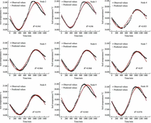
3.1 Temporal variation analysis of each sensor node The monitored data acquired from Node 2 to Node 10 in May 23, 2013 are showed in Figure 2. The average span of daily soil temperature was 4.18°C for all sensor nodes. The lowest temperature usually appeared in the morning during 05:00-07:00, and the highest temperature appeared in the afternoon during 15:00-18:00. The observed soil temperatures were compared with the predicted results by the model described in Equation (1).

November, 2016 Liu H, et al. Spatio-temporal variation analysis of soil temperature based on WSN Vol. 9 No.6 135

In these nine non-linear regressions, R2 values ranged from 0.941 to 0.979. Individual nodes, such as the 2nd,

3rd and 9th nodes, have relatively large prediction

differences due to the effect of topography. But in general one strong correlation was obviously found between the observed values and estimated values of the sinusoidal model at the designing depth in this study. The result indicated that the model well predicted the soil temperature at any time in a day. Moreover, appropriate sampling interval can be chosen according to the characteristics of sinusoidal function. As is known, the soil temperature is directly affected by the depth. However, the influence of the depth was not taken into

account in the model. Therefore, further study is needed to improve the model.

A case in point was the long-term trend analysis for the soil temperature data of Node 3 and Node 4 from May 22, 2013 to June 20, 2013 (Figure 3). In addition, the varied curve of daily average air temperature from the

weather station was plotted for comparison. It showed

similar trends with these curves over time. The result proved the effect of air temperature on the soil temperature. These results were consistent with previous study that daily average soil temperature was estimated by daily average air temperature with linear regression on regional scale[18]_.

Figure 3 Daily average soil temperature of node 3 and Node 4 versus daily average air temperature

3.2 Spatial variation analysis for a certain day

It was found that the spatial variability of soil temperature was weak according to the range of coefficient[19]_{. Daily average soil temperature of each}

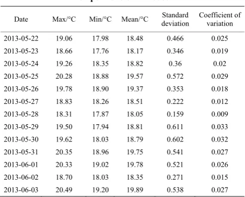
day was proved following a normal distribution before geo-statistics analysis. The statistical values of daily average soil temperature of all nodes for some days are showed in Table 1. The semivariogram curves for the spatial continuity were plotted from the experimental data of May 22, 2013 and June 3, 2013, as shown in Figure 4. The Gaussian model was selected for variogram analysis in the research. Daily average soil temperature of all sensor nodes in May 22, 2013 and June 3, 2013 were processed separately to obtain the corresponding spatial distribution maps (Figure 5) in ArcGIS Geostatistical Analyst Extension. The daily average soil temperature was divided into six distribution levels by using manual classification method aiming to compare the spatio-temporal variation. The threshold values of

levels were set according to the legend of classes. The colors from light to dark in the map represent the daily average soil temperature from low to high, respectively. It is obvious that the spatial distribution of daily average soil temperature fluctuated substantially over time.

Table 1 The statistical values of daily average soil temperature of all nodes

Date Max/°C Min/°C Mean/°C _deviationStandard Coefficient of _variation

2013-05-22 19.06 17.98 18.48 0.466 0.025

2013-05-23 18.66 17.76 18.17 0.346 0.019

2013-05-24 19.26 18.35 18.82 0.36 0.02

2013-05-25 20.28 18.88 19.57 0.572 0.029

2013-05-26 19.78 18.90 19.37 0.353 0.018

2013-05-27 18.83 18.26 18.51 0.222 0.012

2013-05-28 18.31 17.87 18.05 0.159 0.009

2013-05-29 19.50 17.94 18.81 0.611 0.033

2013-05-30 19.62 18.03 18.79 0.602 0.032

2013-05-31 20.35 18.96 19.75 0.541 0.027

2013-06-01 20.33 19.02 19.78 0.521 0.026

2013-06-02 18.70 18.03 18.35 0.271 0.015

a. May 22, 2013 b. June 3, 2013

Figure 4 Semivariogram curves of soil temperature

a. May 22, 2013 b. June 3, 2013

Figure 5 Spatial distribution of daily average soil temperature

3.3 Spatio-temporal variation analysis

The spatial interpolation map could be converted into the vector data, and the area of the various distribution levels were calculated and exported as attribute. Then,

MCDI value can be calculated according to Equation (6). In order to compare the values of MCDI in different days during the experiment, the uniform distribution standard with an equal interval of 0.5°C was used in the spatio-temporal variation analysis. The classes distribution of daily average soil temperatures in May 22 and June 3, 2013 are showed in Table 2. Let MCDI(t1)

denotes MCDI for the first day of this experiment (May

22, 2013), so MCDI for June 3, 2013 is denoted as

MCDI(t13). The values of MCDI(t1) and MCDI(t13) were

calculated as 18.48°C and 19.78°C by Equation (6), respectively. Such values above were found good indicators of daily average soil temperature in the entire region.

Table 2 Monitored classes of daily average soil temperature

Class Range Median

May 22, 2013 June 3, 2013

Area

/m2 Distribution _ratio/% Area _/m2 Distribution _ratio/%

1 (17.5-18.0] 17.75 253.575 1.72 0 0

2 (18.0-18.5] 18.25 7519.614 50.96 0 0

3 (18.5-19.0] 18.75 6967.395 47.22 0 0

4 (19.0-19.5] 19.25 14.969 0.10 4706.861 31.90

5 (19.5-20.0] 19.75 0 0.0 4339.332 29.41

6 (20.0-20.5] 20.25 0 0.0 5709.36 38.69

According to Equation (7), the spatial distribution variation over time ΔMCDI is computed as following:

13 1

( ) ( )

19.78 C 18.48 C 1.3 C

MCDI MCDI t MCDI t

Δ = −

= ° − ° = ° (8)

November, 2016 Liu H, et al. Spatio-temporal variation analysis of soil temperature based on WSN Vol. 9 No.6 137

indicator for planting dates decision-making. The

MCDI is calculated by weighted averaging of each spatial distribution area. It is more representative of the regional soil temperature compared with the usual measurements in single point. Therefore, the critical soil temperature for best planting dates could be real-time monitored by setting the threshold of MCDI or ΔMCDI. The MCDI value is consistently higher than the threshold for the required days, which can be indicated that the regional soil temperature is suitable for sowing.

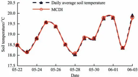
The comparison of the statistical daily average soil temperature of all nodes with the MCDI values from May 22, 2013 to June 3, 2013 is shown in Figure 6. It is found that the two curves are different but very similar at the same day. Thus, it is necessary to perform data validation over a longer period and wider region in the future work.

Figure 6 Comparison of MCDI and statistical daily average soil temperature of all nodes

4 Conclusions

An approach capable of analyzing continuous data from WSN applications is presented based on the classical statistics and geo-statistics in this paper. Three aspects, i.e. temporal variation analysis, spatial variation analysis and spatio-temporal variation analysis were conducted. Methods above were verified by analyzing results of the temporal variation, spatial distribution and spatio-temporal variation of real-time soil temperature data. Temporal variation analysis of each sensor node showed a sinusoidal variation of daily soil temperature and gave a long-term trend of daily average soil temperature in a certain period. The spatial distribution map of daily average soil temperature was provided within a study region by spatial variation analysis. The

changing process of spatial distribution over time was quantified with spatio-temporal variation analysis by

MCDI, an indicator proposed in this study. The

influence of the buried depth of sensors was not taken into account in the model, which need to be further studied to improve the model.

Acknowledgements

This study was supported by National Nature Science Foundation of China (Grant No. 31101078, 31571563, 31571564), National High Technology Research and Development Program of China (Grant No. 2013AA102308) and Scientific Research Common Program of Beijing Municipal Commission of Education (Grant No. KM201410028016).

[References]

[1] Prasad P V V, Boote K J, Thomas J M G, Jr L H A, Gorbet D W. Influence of soil temperature on seedling emergence and early growth of peanut cultivars in field conditions. Journal of Agronomy & Crop Science, 2006; 192(3): 168–177.

[2] Zhang N, Wang M, Wang N. Precision agriculture-a worldwide overview. Computers and Electronics in Agriculture, 2002; 36: 113–132.

[3] Amirinejad A A, Kamble K, Aggarwal P, Chakraborty D, Pradhan S, Mittal R B. Assessment and mapping of spatial variation of soil physical health in a farm. Geoderma, 2011; 160(3-4): 292–303.

[4] Ojha T, Misra S, Raghuwanshi N S. Wireless sensor networks for agriculture: The state-of-the-art in practice and future challenges. Computers & Electronics in Agriculture, 2015; 118: 66–84. DOI: 10.1016/j.compag.2015.08.011 [5] Zhang M, Wang W, Liu C, Gao H, Li M. Development of a

wireless sensor network for soil moisture monitoring in precision agriculture. American Society of Agricultural and Biological Engineers Annual International Meeting 2012, Dallas, Texas, July 29 - August 1, 2012.

[6] Dong X, Vuran M C, Irmak S. Autonomous precision agriculture through integration of wireless underground sensor networks with center pivot irrigation systems. Ad Hoc Networks, 2013; 11(7): 1975–1987.

[7] Li Z, Wang N, Franzen A, Taher P, Godsey C, Zhang H, et al. Practical deployment of an in-field soil property wireless sensor network. Computer Standards & Interfaces, 2014; 36(2): 278–287.

al. Wireless sensor network deployment for monitoring soil moisture dynamics at the field scale. Procedia Environmental Sciences, 2013; 19: 426–435

[9] Vuran M C, Akan O B, Akyildiz I F. Spatio-temporal correlation: theory and applications for wireless sensor networks. Computer Networks, 2004; 45: 245–259.

[10] Heathman G C, Cosh M H, Han E, Jackson T J, McKee L, McAfee S. Field scale spatiotemporal analysis of surface soil moisture for evaluating point scale in situ networks, Geoderma, 2012; 170: 195–205

[11] Zhang M, Li M, Wang W, Liu C, Gao H. Temporal and spatial variability of soil moisture based on WSN. Mathematical & Computer Modelling, 2013; 58(3-4): 826–833.

[12] Liu H, Meng Z J, Xu M, Shang Y Y. Sensor nodes deployment based on regular patterns in farmland environmental monitoring. Transactions of the CSAE, 2011; 27(8): 265–270. (in Chinese with English abstract)

[13] Rains G C, Thomas D L, Vellidis G. Soil-sampling issues for precision management of crop production. Applied Engineering in Agriculture, 2001; 17(6): 769–775.

[14] Webster R, Oliver M A. Chapter 4. Characterizing spatial

processes: The Covariance and Variogram. Geostatistics for Environmental Scientists, Second Edition. John Wiley & Sons, Ltd, 2008; pp. 47–76.

[15] Fischer M M. Handbook of Applied Spatial Analysis Handbook of applied spatial analysis: Springer, 2010; pp. 27–41.

[16] Cui X W, Zhang L, Zhu L, Song G, Wu B. Changes of landscape pattern and its characteristics in Kaixian county before and after impoundment of Three Gorges Dam Project. Transactions of the CSAE, 2012; 28(4): 227–234. (in Chinese with English abstract)

[17] Zeng Y N, Jin W P, Wang H M, Zhang H. Simulation of land-use changes and landscape ecological assessment in eastern part of Qinghai Plateau. Transactions of the CSAE, 2014; 30(4): 185–194.

[18] Awe G O, Reichert J M, Wendroth O O. Temporal variability and covariance structures of soil temperature in a sugarcane field under different management practices in southern Brazil. Soil & Tillage Research, 2015; 150: 93–106.