Munich Personal RePEc Archive
A new test for deficit sustainability and
its application to US data
Hatzinikolaou, Dimitris and Simos, Theodore
University of Ioannina
14 August 2011
ACCEPTED BY EMPIRICAL ECONOMICS
A new test for deficit sustainability and its application to US data
Dimitris Hatzinikolaou
and Theodore Simos*
Abstract In this paper, we define deficit sustainability by requiring formally that
both the discounted debt vanish asymptotically and the undiscounted debt be bounded. Thus, a new necessary condition and a new testing procedure emerge. We propose a new test statistic and prove that its limiting distribution is standard normal,
N(0, 1). Its finite- sample distribution differs from N(0, 1), however, mainly because it has fat tails, so we derive empirical critical values using simulations. Using the new test and United States (US) quarterly data, the conclusions of three earlier papers that fail to reject the sustainability of the US budget or current-account deficit are reversed.
Keywords Undiscounted debt, budget, current account, sustainable.
JEL Classification E62, H62, H63.
1
1 Introduction
Many economists consider the budget deficit to be “too large,” and therefore
unsustainable, not only when the government´s intertemporal budget constraint (IBC)
is violated, but also when the IBC is satisfied, but for each dollar of government
spending (inclusive of interest payments) revenue rises by less than one dollar
(Hakkio and Rush 1991, p. 433; Tanner and Liu 1994, p. 514; Haug 1995, p. 106;
Quintos 1995, p. 410; and Payne 1997, p. 777). In that case, it is argued, the
government may have difficulty in marketing its debt in the long-run, and may thus
have an incentive to default on it or use inflationary finance. The reason is that,
although the present discounted value of the debt tends to zero (and so the IBC is
satisfied), the undiscounted value of the debt may tend to infinity. The same argument
is used in the case of the current-account deficit (Husted 1992, footnote 2; Wu et al.
1996, p. 194; Wu et al. 2001, p. 220; and Holmes 2006, p. 629). Surprisingly,
however, although this argument imposes a testable condition, the only conditions
tested formally in the literature are those implied by the IBC.
This paper defines sustainability by requiring formally that both the discounted
debt converge to zero and the undiscounted debt be bounded. Thus, a new necessary
condition and a new testing procedure emerge. We propose a new test statistic and
prove that its limiting distribution is standard normal, N(0, 1). For sample sizes
encountered in practice, however, its distribution differs from N(0, 1), mainly because
it has fat tails, so we derive empirical critical values using Monte-Carlo simulations.
The proposed test is more stringent than the standard one, as it requires that an
additional condition be satisfied. It seems appropriate, however, in view of Bohn´s
(2007) criticism that “standard unit root and cointegration tests are incapable of
2
imposes very weak econometric restrictions” (p. 1846). That is, according to this
criticism, the traditional tests for sustainability, which exploit only the conditions
implied by the IBC, e.g., Wilcox (1989), Hakkio and Rush (1991), and Trehan and
Walsh (1991), reject sustainability less often than they should.
After setting up the model (Section 2), we derive the new condition and the new
test (Section 3), and explain how we obtain the empirical critical values by Monte-
Carlo simulations (Section 4). Using this approach and United States (US) quarterly
data, Section 5 demonstrates that the conclusions of three papers that fail to reject the
sustainability of the US budget or current-account deficit are reversed. In particular,
using the alternative sample periods and deficit measures considered in these papers,
the new test rejects sustainability in almost every case. Interestingly, however, when
we use our own sample period, 1947.1-2010.1, the test does not reject sustainability
of the US current-account deficit. Section 6 concludes the paper.
2 The model
Following Hakkio and Rush (1991), we begin by considering the government´s
one-period budget constraint in real terms:
Gt + itBt-1–Rt = ΔΒt, (1)
where Gt = government purchases of goods and services plus transfer payments, Rt =
revenue, it = interest rate, Bt = market value of the debt, and ΔΒt = Βt –Βt-1. Assuming
that the real interest rate is stationary around a constant mean, i; and adding and
3
Gt + (it – i)Bt-1 is “adjusted spending” (Bohn 2007, p. 1839). Solving this equation
forward and letting β = 1/(1+i) yields the IBC:1
j t j
j
j t j t j
j
t R A B
B 1
0 1
1 ( ) lim . (2)
The last term of Eq. (2) disappears after imposing the “no Ponzi game condition”
(NPG), i.e., lim[ + /(1+ ) +1]=0
j j
t
j→∞ B i , which says that the discounted debt must
converge to zero in the indefinite future. Thus, Eq. (2) essentially says that real
government debt outstanding equals the present value of (expected) future primary
surpluses.2 Note that a necessary and sufficient condition for the NPG condition to
hold is that the rate of growth of the numerator (Bt+j), denoted as gB, be smaller than i,
which is the rate of growth of the denominator, (1+i)j+1. As Cuddington (1997, p. 8)
notes, this condition (i.e., gB < i) is usually justified on the grounds that lenders would
presumably refuse to buy government debt if the government perpetually issued new
debt to pay its entire current interest obligation [i.e., if ΔΒt = itBt-1, hence Rt –Gt = 0,
using Eq. (1)], instead of running primary surpluses (Rt – Gt > 0). If lenders were
willing to buy such debt when Rt+j– Gt+j = 0 for all j, then Eq. (1) implies that gB =
ΔΒt/Bt-1 = i, not gB < i, and thus the NPG condition fails.
To derive testable restrictions, rewrite Eq. (2) as follows:3
h t h
h
h t h t h
h t
t R R A B
GG 1 ( ) (1 )lim , (3)
1 At this point, one might consider introducing expectations, as in Martin (2000, p. 85). By doing so,
however, the test statistic derived below would depend on expected deficits and, to make it operational, the deficit process would have to be modeled. For the purposes of the present paper, however, the expectations operator can be omitted, as the econometrician uses historical data in order to judge whether a sequence of realized deficits has been on a sustainable path. Note also that Hakkio and Rush (1991, p. 432, footnote 5) argue that it is not strictly correct to take expectations of an accounting identity, Eq. (1), in order to arrive at a stochastic version of the IBC, Eq. (2), since Eq. (1) must hold for all values of the variables, not just for the average ones.
2 Since R
t–At = Rt–Gt– (it–i)Bt-1 and, on average, it–i = 0 (because the mean of it is i), we have, on
average, that Rt–At = Rt–Gt. If Rt–Gt > 0 (< 0), this number is called primary surplus (deficit).
4
where GGt = Gt + itBt-1. Assuming that Rt and At are each a random walk with a drift,
i.e., Rt α1 Rt 1 ε1t and At 2 At 1 2t, and that the NPG condition is
satisfied, Eq. (3) leads to the following regression equation:
t t t α bGG ε
R , (4)
where a = (α2 – α1)/i and εt Σh 1βh(ε2t ε1t). The usual null hypothesis of deficit
sustainability is that εt is stationary, i.e., that Rt and GGt are cointegrated,4 and that
the systematic relationship between these two variables is one-to-one, i.e., b = 1; no
restrictions on a are tested.5
To obtain an expression for the undiscounted debt, substitute (4) into (1); assume
that it = i for all t; and rearrange, to get Bt (St εt) γBt 1, where γ = 1 + (1 – b)i
and St (1 b)Gt a. Iterating this difference equation for Bt forward yields6
1 1
, t
j j t j
t Ψ B
B , (5)
where
j
k t k t k
k j j
t S
Ψ , 0 ( ). (6)
Note that, from a pragmatic point of view, e.g., considering the marketability of
government debt, meeting the Maastricht conditions, etc., sustainability requires that
4 Bohn (2007) does not restrict the variables R
t and GGt to be I(1), and concludes that sustainability
does not require that these two variables be cointegrated. In this paper, the requirement that the two variables be cointegrated is retained for the cases where Rt and GGt are both I(1).
5 Martin (2000, p. 86) summarizes nicely the existing terminology regarding sustainability: The deficit
is said to be strongly sustainable if and only if there is cointegration in Eq. (4) and b = 1; it is only
weakly sustainable if there is cointegration and 0 < b < 1; and it is unsustainable if b 0.
6 An error that occurred in Hakkio and Rush (1991, p. 433) may be a source of confusion. Hakkio and
Rush substitute aˆ bˆGGt for Rt in Eq. (1) and iterate forward to obtain the undiscounted value of the
debt. Setting the actual value of Rt equal to its fitted value from regression (4), however, has the effect
of ignoring temporary changes in taxes, which are reflected in the residuals, et. That is, in the Hakkio
and Rush paper, the quantity St should be replaced by St– et. Here, we have St– εtinstead, as we
5
the undiscounted debt, given by Eq. (5), be bounded. Is this criterion stronger than the
NPG condition? Cuddington (1997, p. 13) answers yes, provided that the real interest
rate (i) exceeds the rate of growth of real GDP (gY), i.e., i > gY. He explains this by
assuming that i > gB > gY, where gB = ΔΒt/Bt-1. The first part of this inequality (i > gB)
is a requirement for the NPG condition to hold [see the discussion following Eq. (2)],
whereas the second part (gB > gY) can hold when fiscal policy dominates monetary
policy and the monetary authority tries to fight inflation, thus letting the real stock of
government debt held by the public grow (Sargent and Wallace 1981, p. 2). Under
these circumstances, since i > gB, the NPG condition is satisfied, but the debt-to-GDP
ratio is unbounded, as gB > gY. That is, the NPG condition does not imply boundedness
of the debt-to-GDP ratio. Next, suppose that the debt-to-GDP ratio is bounded, i.e., gB
≤ gY. Combining this condition with the condition i > gY (assumed above) yields i > gB,
which implies that the NPG condition is satisfied. Therefore, under the above
assumptions, the boundedness of the debt-to-GDP ratio is a stronger condition than
the NPG condition, as the former implies the latter, but not vice versa.
Hakkio and Rush (1991) argue that as j → ∞, Bt+j → ∞ when b < 1, apparently
because in that case γ > 1 [assuming i > 0 in γ = 1 + (1 –b)i], and thus the second term
on the right-hand side of Eq. (5) tends to infinity (assuming Bt-1 > 0). This argument
considers only the initial debt (Bt-1), however, and neglects subsequent deficits or
surpluses, which are included in the first term of Eq. (5), Ψt,j. The next section
6
3 A testing procedure
Consider the term St k t k in the definition of Ψt,j, Eq. (6). Since
a G b
St (1 ) t and t Rt a bGGt [Eq. (4)], where GGt Gt itBt 1; and
since we have assumed that it = i for all t; it follows that
) (
1 t t t
t
t ε biB R G
S . (7)
Thus, St εt is the difference between the part of the interest outlay that is returned
to the government as taxes,7 biBt 1,and the primary budget surplus, Rt Gt. Adding
and subtracting iBt 1 to the right of Eq. (7) yields
St εt (Gt iBt 1 Rt) (1 b)iBt 1. (8)
Thus, St εt is also the difference between the budget deficit (inclusive of interest),
,
1 t t
t iB R
G and the part of the interest outlay that does not accrue to the
government as taxes, (1 b)iBt 1.
In Appendix A, we prove the following proposition, which leads us to the testing
procedure expounded below.
Proposition: If we define deficit sustainability by requiring formally that both the
discounted debt vanish asymptotically and the undiscounted debt be bounded, then
(a) a necessary condition for sustainability is
0
,j t
Ψ ; (9)
(b) under cointegration and b = 1, (9) is also a sufficient condition;
(c) under cointegration and b = 1, another necessary and sufficient condition is a ≥ 0;
(d) under cointegration and b < 1,the condition a > 0 is necessary, but not sufficient.
7 The observation that the government´s interest payments become households´ income part of which
7
Remark 1: In part (c), necessity implies that if a is statistically significantly
negative, then we should reject sustainability. In some applications, however, there
might arise the issue of statistical versus practical significance: a small negative value
of a implies a positive value for Ψt,j (when b = 1), but this value may be too small to
realistically consider the undiscounted debt to be too large. Thus, we should test the
largeness of Ψt,j directly by testing (9), instead of testing the condition a≥ 0.
Remark 2: As the proof of part (d) makes clear (see Appendix A), when b < 1, the
additional condition for sustainability that should be tested is not a≥ 0, but Ψt,j 0.
Although the latter condition is not sufficient either when b < 1, it is nevertheless
more conclusive than the condition a≥ 0.
An intuitive explanation of condition (9) is as follows. Given the interpretation of
the difference St εt based on Eq. (7), condition (9) says that sustainability requires
that, on the average, the primary surplus be at least as great as the part of the interest
outlay that is returned to the government as taxes, so it can be used to finance part of
the interest payments on the debt. If so, the deficits may be considered sustainable and
the undiscounted debt bounded, thus attenuating expectations of default; and this
policy can go on for many years, without a need for the government to default on its
debt or to inflate.8
Note that the discussion so far refers to the budget deficit, but it can be adapted
easily for the case of the current-account deficit. In this case, the symbol GG may be
interpreted as real imports of goods and services plus income payments plus real taxes
8 This observation is consistent with McCallum´s (1984) famous theoretical result that in a
8
and transfers paid to the rest of the world (net), and R as real exports of goods and
services plus income receipts from the rest of the world.
The foregoing discussion suggests the following testing procedure. Using Eq. (4),
test the hypotheses of cointegration and H0: b = 1, a = 0 and consider the following
cases:
1. Cointegration and H0 are not rejected. In this case, do not reject sustainability.
2. Cointegration is rejected. In this case, reject sustainability.
3. Cointegration is not rejected, but H0 is rejected. In this case, test the following
two hypotheses separately: (i) H0: b≥ 1 against H1: b < 1; and (ii) H0: a ≥ 0
against H1: a < 0. There are three possible outcomes:
3a. If both hypotheses (i) and (ii) are rejected, reject sustainability.
3b. If (i) is not rejected, but (ii) is rejected, test condition (9); if it is rejected,
reject sustainability; but if it is not rejected, do not reject sustainability.
3c. If (i) is rejected, but (ii) is not rejected, test condition (9); if it is rejected, reject
sustainability; but if Ψt,j is significantly negative, do not reject sustainability.
In this procedure, it is crucial to take into account structural breaks, since they
affect both the test for cointegration and the tests on the values of the parameters a
and b. Wilcox (1989, p. 292 and 300), Trehan and Walsh (1991, pp. 215-216 and
220), Tanner and Liu (1994, pp. 513-517), and Husted (1992, pp. 163-165) report
evidence of structural breaks, so the choice of sample period is important.
To test condition (9), an appropriate test statistic (TS) must be constructed, whose
distribution can be approximated under the joint hypothesis of cointegration and H0: b
= 1, a = 0. In Appendix A, we prove the following theorem, which is the main
9
Theorem: Under the joint hypothesis of cointegration and H0: b = 1, a = 0, the
interest-inclusive real deficit, ds, is a zero-mean stationary process; if ds is also an
ergodic process satisfying “Gordin’s condition,” then
) 1 , 0 ( , N v T Ψ TS d j t
, (10)
where Ψt,j is defined in Eq. (6), T is the sample size, v j λj, and λjis the
autocovariance of ds between the dates s and s–j.
An important issue that needs to be addressed at the outset when implementing the
test statistic TS given in (10) is the estimation of the value of v j j. As is well
known, λj λ j, so v 0 2 j 1 j 2 sds(0), where 0 is the variance and
) 0 ( s
d
s is the spectrum of the series ds at frequency zero [Hamilton 1994, p. 153, Eq.
(6.1.6)]. Thus, letting a hat (^) denote an estimator, we obtain
) 0 (
ˆ
2
ˆ sds
v . (11)
In this paper, we use two estimators of sds(0) in Eq. (11), thus obtaining two
estimators of v. First, we use a popular estimator of the spectrum, which employs the
Bartlett kernel, so the estimator of sds(0) is given by
} ˆ )] 1 /( 1 [ 2 ˆ { ) 2 ( ) 0 (
ˆ 0 1
1 q
j j
s
d j q
s , (12)
where q is a suitably chosen number [Hamilton 1994, p. 167, Eq. (6.3.15)]. Here, we
adopt the choices q = T1/5, q = T1/3, and q = T2/5, as they have been found to be optimal
in certain settings (Xiao and Phillips 1998).
Our second estimator of v avoids the problem of choosing a value for q. In this
case, we estimate an ARMA(p, q) model for the stationary series ds,
q t q t t p t s p t s t
s c d d u u u
10
where ut is a white-noise process with variance σ2; obtain estimates of σ2, υ1, ..., υp,
θ1, ..., θq; calculate the value of sˆds(0) using the formula
2 1
2 1
2
)
ˆ
...
ˆ
1 (
)
ˆ
...
ˆ
1 ( 2 ) 0 (
ˆ
p q ds
s (14)
[Hamilton 1994, p. 155, Eq. (6.1.14)]; and substitute this value in (11).
4 Monte-Carlo simulations
A more important issue that also needs to be addressed is whether the finite-sample
distribution of TS is adequately approximated by the N(0, 1) distribution. Our
Monte-Carlo (MC) simulations (with 50,000 replications) show that, for the sample sizes
encountered in practice, the distribution of TS is symmetric in most cases, but always
exhibits kurtosis of various degrees, in most cases in the form of somewhat fatter tails
than those of the N(0, 1) distribution. For example, using Eq. (12) as an estimator of
the spectrum and the sample sizes considered in this paper (T = 253, 160, 104, 103,
and 92), in 68 percent of the MC experiments that we have carried out symmetry is
not rejected (at the 10-percent level), whereas kurtosis is strongly rejected (at the
1-percent level) in every case. Thus, the Jarque-Bera test strongly rejects normality (at
the 1-percent level) in every case, with values ranging from 100 to 12660. These
rejections are even stronger when we estimate the spectrum by Eq. (14), since in these
experiments symmetry is also strongly rejected in every case. Note also that we have
carried out some MC experiments with sample sizes larger than T = 253, e.g., T =
500, 1000, 1500, and 2000. In these cases, as the value of T increased, the empirical
distributions of the statistic TS approached the N(0, 1) distribution, but the
11
This evidence shows that, for realistic sample sizes, the critical values from the
N(0, 1) distribution are inappropriate, and we must compute empirical critical values
for TS by MC simulations. When doing so, we should bear in mind that the test is
right-sided. Note also that, as the following paragraphs will make clear, these critical
values are not generic, but depend on the specific data sets used in this paper.
Our MC simulations that use Eq. (12) as an estimator of the spectrum consist of
the following steps. First, we use actual data for the deficit series, for which we have
found evidence that it is I(0), to estimate a parsimonious ARMA(p, q) model that
includes a constant term, i.e., Eq. (13). We choose the “best” model using the
following criteria: (i) satisfaction of the standard stationarity conditions (Hamilton
1994, Chapter 3); (ii) statistically significant coefficients at conventional levels; (iii)
absence of serial correlation at the 10-percent level, according to the Ljung-Box test;
and (iv) maximization of 2
R by over-fitting and under-fitting autoregressive and
moving average terms.
Second, we use the estimates of σ2, υ1, ..., υp, θ1, ..., θq obtained from the first step
to generate 50,000 “samples” of size T for a zero-mean stationary series ds. Note that
T takes on the same values as those we have in our actual data, and that each “sample”
consists of T random numbers taken from the normal distribution with mean zero and
variance the estimate of σ2 obtained from the first step.
Third, for each “sample” we calculate the value of TS by substituting the values of
T
Ψ1, and ˆj obtained from this “sample.” Fourth, we construct the frequency
distribution of these 50,000 values of TS, from which we obtain the 1%, 5%, and 10%
empirical critical values as the 99%, 95%, and 90% fractiles of this distribution.
Alternatively, when we estimate the spectrum by Eq. (14), our MC simulations
12
from the generated zero-mean stationary series ds, we re-estimate the same ARMA(p,
q) model, with the restriction c = 0 imposed on Eq. (13), and then use the resulting
estimates of σ2, υ1, ..., υp, θ1, ..., θq in Eq. (14).
In Tables 4 and 5, we report the 1%, 5%, and 10% empirical critical values from
the MC simulations along with the estimated values of TS obtained from the actual
data. We do not report the critical values in a separate table, because, as we mentioned
earlier, they cannot be used generally, i.e., for other data sets.
5 Application of the new test to the US budget and current-account deficits
Using the new test and US quarterly data, 1947.1-2010.1 (see Appendix B), this
section shows that some of the existing results in the literature can be reversed if, in
addition to the standard restrictions for sustainability (implied by the IBC), we require
formally that the undiscounted debt be bounded. In particular, we consider the paper
by Tanner and Liu (1994) on the sustainability of the US budget deficit, and the
papers by Husted (1992) and Wu et al. (2001) on the sustainability of the US
current-account deficit. These authors use various deficit measures and sample periods.
For each deficit measure and sample period considered in these papers, we have
carried out our own unit-root and cointegration tests. As unit-root tests, we use the
following: (1) the ADF test of Dickey and Fuller (1981); (2) the KPSS test of
Kwiatkowski et al. (1992); (3) the MSB test of Ng and Perron (2001); and (4) the Lee
and Strazicich (2003, 2004) test, which allows for one or two structural breaks. Our
results from these tests differ somewhat from those of the above three papers, in that
some series, which were taken to be I(1) there, turn out to be I(0) here,9 mostly
9 Whenever there is evidence that the variables involved are I(0), a more appropriate term than
“cointegration” is a “levels relationship”; see Pesaran et al. (2001). Of course, the test has been derived
13
because we use the Lee-Strazicich test. For the purposes of the present paper,
however, we shall treat the results of the above three papers on unit roots as correct.
The main reason why we have carried out our own unit-root tests was to check the
assumption of deficit stationarity, which is necessary for the application of the test.
Please insert Tables 1 and 2 here
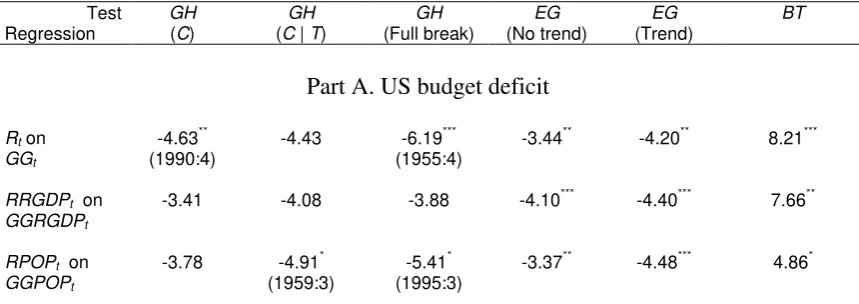
As cointegration tests, we use the following: (1) the Engle and Granger (1987)
test; (2) the Gregory and Hansen (1996a, 1996b) tests; and (3) the Pesaran et al.
(2001) “bounds test.” Our results are similar to those of the above authors, in that we
find cointegration in every sample period considered, although in a few cases the
evidence is weak. For space considerations, we report the results on unit-root and
cointegration tests only for the full-sample period, 1947.1-2010.1 (see Tables 1-3).10
Please insert Table 3 here
We now turn to the application of the new test to the sample periods used by the
three papers mentioned above as well as to the full-sample period. First, consider the
results of Tanner and Liu (1994) for the US budget deficit. By using the IBC criterion
and by allowing for a structural break in 1982:1, these authors cannot reject the
hypotheses of cointegration and b = 1 for the sample periods 1950-1989 and
1964-1989. Thus, they conclude that sustainability holds, despite the evidence that the value
of the parameter a has become significantly negative after 1982:1 (see their Table I).
assumed that they are AR(1) processes, i.e., Rt 1 1Rt 1 1t and At 2 2At 1 2t, where
| i | < 1, i = 1, 2, then, by adding Rt-1–Rt-1 = 0 to the first and At-1–At-1 = 0 to the second of these two
equations, we can write them as Rt 1 Rt 1 1*t and
* 2 1 2 t t
t A
A , where
1 1 1 *
1t t ( 1)Rt and 2*t 2t ( 2 1)At 1. The only effect on Eq. (4) is that its error term is
now defined as 1 [ 2t 1t ( 2 1) t 1 ( 1 1) t 1]
h h
t A R . This is a stationary variable, as ε1t,
ε2t, Rt, and At are all assumed to be stationary. To the extent that it is also a zero-mean and ergodic
process satisfying Gordin’s condition, the test is applicable.
10 The results for the sub-sample periods and for the alternative current-account deficit measures
14
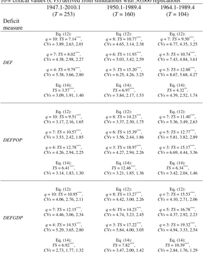
Using the new test procedure, however, the conclusion of the Tanner and Liu
(1994) paper, which falls into Case 3b, is reversed. For each of the two sample
periods used by these authors, as well as for the full-sample period, 1947.1-2010.1,
we calculate the value of the test statistic (10), TS, for the following three measures of
the real budget deficit (inclusive of interest), ds: (a) in levels (DEF), (b) in per capita
terms (DEFPOP), and (c) in percent of real GDP (DEFGDP). For each deficit
measure and each sample period, we use four estimates of the spectrum at frequency
zero to calculate the values of TS and empirical critical values by MC simulations
with 50,000 replications. Table 4 reports the results. For the three sample periods and
the three budget-deficit measures considered, sustainability is rejected in every case at
the 5-percent level, and in 35 out of 36 cases at the 1-percent level.
Please insert Table 4 here
Second, consider the results of Husted (1992) and Wu et al. (2001) on the
sustainability of the US current-account deficit. These authors report evidence
favoring the hypotheses of cointegration and b = 1 in Eq. (4). Thus, Wu et al. (2001,
p. 223) conclude explicitly that the US current-account deficit can be considered
sustainable, whereas Husted (1992) does so only implicitly, since he adopts the
Hakkio and Rush (1991) criteria for sustainability (see his footnote 2).
Using our test, sustainability is rejected, however, because there is evidence
against condition (9). Note that the results of Husted (1992) are more relevant, since
he uses time-series data from the US, 1967.1-1989.4, whereas Wu et al. (2001) use
panel data from the G7 countries for the period 1973.2-1998.4.11
11 Using the Hakkio and Rush (1991) criteria and panel data from 11 countries, including the US, for
15
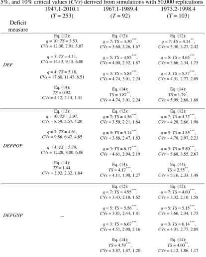
For each of the sample periods used in these two papers, as well as for the
full-sample period, 1947.1-2010.1, we calculate the values of TS for the following three
deficit measures: (a) in levels (DEF), in per capita terms (DEFPOP), and (c) in
percent of real GNP (DEFGNP), where the word “deficit” now means real current
-account deficit, inclusive of income receipts and payments as well as current taxes and
transfers to the rest of the world. Table 5 reports the results. For the sample periods
considered in the above two papers, 1967.1-1989.4 and 1973.2-1998.4, sustainability
can be rejected in every case. In particular, at the 1-percent level, it is rejected in 19
out of 24 cases; at the 5-percent level, it is rejected in 23 out of 24 cases; and at the
10-percent level, it is rejected in every case. Interestingly, however, sustainability is
not rejected for the full sample period, 1947.1-2010.1. Note also that for this sample
period we do not report results for DEFGNP, because the unit-root tests suggest that
this variable behaves as an I(1) process, so our test is not applicable.
Please insert Table 5 here
Note that the results reported in Table 2C of Husted (1992) are similar to those of
Tanner and Liu (1994) described earlier, so their interpretation should be the same.
By allowing for a structural break in 1983:4, Husted (1992) finds that the hypotheses
of cointegration and b = 1 cannot be rejected, but the value of the parameter a has
become significantly negative after 1983:4. Thus, Husted’s (1992) paper also falls
into Case 3b of the approach proposed here. Husted (1992, p. 165) concludes that
after 1983:4 “the long-run tendency of the current account balance has shifted from
zero to a deficit in excess of $100 billion per year,” but implicitly considers (along
16
with the cited literature) the deficit to be sustainable, since he adopts the Hakkio-Rush
criteria. The evidence presented here points to the opposite conclusion, however.
Finally, consider the evidence when the current-account deficit is measured as in
Husted (1992), i.e., by excluding income payments from imports and income receipts
from exports. For the sample period 1967.1989.4, sustainability is rejected at the
1-percent level in 11 out of 12 cases (alternative definitions of the deficit and alternative
estimates of the spectrum), and is rejected at the 5-percent level in every case. As for
the sample period 1973.2-1998.4, we obtain similar rejections only for the deficit
measures DEFPOP and DEFGNP, whereas for DEF we can reject sustainability only
when we estimate the spectrum by Eq. (14). For space considerations, however, we do
not report the values of TS and the empirical critical values for these alternative
current-account deficit measures.12
6 Summary and conclusions
The standard conditions tested in the literature on deficit sustainability emerge from
the requirement that the discounted debt vanish asymptotically. Econometric tests
usually confirm these conditions. But whenever each additional dollar of government
expenditure (inclusive of interest) is systematically accompanied by additional
revenue that is less than one dollar (i.e., whenever b < 1), researchers invoke
informally another criterion, namely, boundedness of the undiscounted debt, and
conclude that in these cases the deficit may not be sustainable.
This paper defines sustainability by requiring formally that both the discounted
debt vanish asymptotically and the undiscounted debt be bounded. This definition
gives rise to a new necessary condition for sustainability and a new testing procedure,
17
which is more stringent than the standard one, as it requires that an additional
condition be satisfied. We propose a new test statistic and prove that its limiting
distribution is standard normal, but in finite samples its distribution differs from the
standard normal, mainly because it has fat tails. Thus, we derive empirical critical
values using Monte-Carlo simulations with 50,000 replications.
Using this approach, the conclusions of three papers that fail to reject the
sustainability of the US budget or current-account deficit are reversed. Conclusions
against sustainability could potentially also be reversed if the hypothesis (i) H0: b≥ 1
is rejected, but the hypothesis (ii) H0: a ≥ 0 is not rejected and Ψt,j is significantly
negative (Case 3c of the proposed testing procedure).
This discussion points to the importance of Eq. (5), which shows how the
undiscounted debt is determined at a given point in time. The paper focuses on the
first term on the right-hand side of this equation, Ψt,j, which has been neglected in
the literature. This term can be positive and contribute to the largeness of the
undiscounted debt, independently of the second term, [1 + (1 – b)i]j+1Bt-1; or be
negative and mitigate (or even offset) the growth of the second term (when b < 1).
That is, the level of the initial debt (Bt-1) and the value of b are not the only factors
that should be taken into consideration by potential lenders who look at the value of
the undiscounted debt; it is also important to look at the value of Ψt,j. For example, if
Bt-1 > 0 and b < 1, and so the second term grows, but from period t onward the
government runs primary surpluses that are (on average) at least as great as the part of
the interest outlay that is returned to the government as taxes, it will be able to finance
part of the interest payments on the debt. Therefore, its lenders may consider the
deficits small and sustainable and the undiscounted debt bounded, thus continuing to
18
Appendix A: Proofs
Proof of the Proposition
(a) Suppose that (9) does not hold, and let Ψt,j be a statistically significant positive
number. Assume also that Bt-1 is positive and large, for otherwise no issue of
sustainability should arise. It follows from Eq. (5) that the undiscounted debt (Bt+j) is
a significantly large positive number, and thus the deficit is unsustainable. Thus, (9) is
necessary for sustainability.
(b) If in addition to cointegration and b = 1 in (4) condition (9) also holds, then the
undiscounted debt is bounded, because the first term on the right of Eq. (5) is either
zero or negative [in accordance with (9)] and the second term is not growing, as γ = 1
(since b = 1).
(c) To prove necessity, assume cointegration and b = 1, so Eqs. (4) and (8) yield
t t
t ε a ε
S , and suppose that a < 0. Since εt has mean zero, this equation
implies that the difference St εt will be systematically positive, hence Ψt,j 0, i.e.,
(9) will be violated. Thus, sustainability requires that a≥ 0.13, 14 To prove sufficiency,
assume cointegration and b = 1, and suppose that a ≥ 0. Using again the equation
t t
t ε a ε
S , where εt has mean zero, the restriction a ≥ 0 implies that St εt
will be a non-positive number, hence Ψt,j 0, i.e., the first term on the right of Eq.
(5) is either zero or negative. And since the second term is not growing, as γ = 1
(because b = 1), it follows that that the undiscounted debt is bounded.
13 It is obvious from Eq. (5) that if sustainability merely requires that the IBC be satisfied, but does not
require that the undiscounted debt be bounded, then the condition a ≥ 0 is not necessary; see also
Tanner and Liu (1994, p. 513).
14 The inequalities a≥ 0 and 0
,j t
19
(d) Assuming cointegration and b < 1, and substituting Eq. (4) into (8) yields
t t
t
t ε a ε b G
S (1 ) . From this equation it is clear that in order for the
difference St εt to be systematically negative, hence Ψt,j 0, it is necessary that a
> 0. In this case (i.e., when b < 1), the condition a > 0 is not sufficient, however. For
if the value of a is positive, so that –a < 0, but not large enough in size to outweigh
(on average) the positive term (1 – b)Gt, then it is possible that the difference St εt
might be systematically positive, hence Ψt,j 0, and sustainability might fail. This
completes the proof of the proposition.
Proof of the Theorem
Under the joint hypothesis, the interest-inclusive real deficit, ds = Gs+ iBs-1 –Rs, is a
zero-mean stationary process, since Eq. (4) reduces to ds εs and εs is a zero-mean
stationary (but likely to be highly autocorrelated) process. Let d be the sample mean
of ds. If the process {ds} is also ergodic satisfying “Gordin’s condition,”15 then by
Gordin’s central limit theorem for zero-mean ergodic stationary processes (Hayashi
2000, p. 404), we have that T d N(0,v),
d
and hence d/ v/T N(0,1)
d
. But,
under the joint hypothesis, γ = 1 and Ψt,j kj 0dt k [by Eq. (8)]. Re-indexing in the
last sum (by substituting t = 1, j = T, and s = k + 1) yields Ψ1, T1d Td,
s s
T and
thus d Ψ1,T /T. Substituting this in the above result yields Ψ1, / Tv N(0,1)
d
T ,
and the proof is complete.
15 A stationary process {y
t} is ergodic if any two of its elements that are sufficiently far apart in the
sequence are almost independent. Gordin’s condition consists of three parts: (a) the process {yt} has
finite second moments; (b) as m , assuming that the unconditional mean of yt is zero, E(yt) = 0, the
conditional expectation E(yt | yt-m) converges to zero in a mean squared error sense; and (c) shocks that
occurred in the distant past do not exert a large effect on the current value of the process, yt. See
20
Appendix B: The data
The data have been obtained from the US Department of Commerce: Bureau of
Economic Analysis, National Income and Product Accounts. They are expressed in
billions of dollars in constant prices of the year 2005 and are seasonally adjusted. In
the case of the budget deficit, the data refer to the Federal Government, where Gt =
purchases of consumption and investment goods and services (deflated by its own
price deflator) plus transfer payments (deflated by the GDP deflator), iBt-1 = interest
payments (deflated by the GDP deflator), and Rt = receipts (deflated by the GDP
deflator). The real budget deficit is defined as DEFt = Gt + iBt-1–Rt = GGt–Rt. In per
capita and in percent of real GDP (RGDP) terms, it is defined as DEFPOPt =
DEFt/POPt and DEFGDPt = DEFt/RGDPt, respectively, where POPt is US
population (in thousands, mid-period).
In the case of the current-account deficit, Mt = imports of goods and services plus
income payments plus net taxes and transfers to the rest of the world (deflated by a
price deflator for imports) and Xt = exports of goods and services plus income receipts
(deflated by a price deflator for exports). In this case, the real current-account deficit
is defined as DEFt = Mt – Xt, DEFPOPt = (Mt – Xt)/POPt, and DEFGNPt = (Mt –
Xt)/RGNPt, where RGNP is real GNP.
Acknowledgments An earlier version of the paper was presented at the Department
21
References
Bohn H (2007) Are stationarity and cointegration restrictions really necessary for
intertemporal budget constraint? J Monetary Econ 54:1837-1847
Box GEP, Jenkins GM (1976) Time series analysis: forecasting and control. Holden
Day, Oakland, CA
Cuddington JT (1997) Analyzing the sustainability of fiscal deficits in developing
countries. The World Bank, International Finance Division, Policy Research
Working Paper 1784
Dickey DA, Fuller WA (1981) Likelihood ratio statistics for autoregressive time-series
with a unit root. Econometrica 49:1057-72
Engle RF, Granger CWJ (1987) Cointegration and error correction: representation,
estimation, and testing. Econometrica 55:251-276
Gregory AW, Hansen BE (1996) Residual-based tests for cointegration in models with
regime shifts. J Econometrics 70:99-126(a)
Gregory AW, Hansen BE (1996) Tests for cointegration in models with regime and
trend shifts. Oxford B Econ Stat 58:555-560(b)
Hakkio CS, Rush M (1991) Is the budget deficit “too large?” Econ Inq 29:429-445 Hamilton JD (1994) Time Series Analysis. Princeton University Press, Princeton
Haug AA (1995) Has federal budget deficit policy changed in recent years? Econ Inq
33:104-118
Hayashi F (2000) Econometrics. Princeton University Press, Princeton
Holmes MJ (2006) How sustainable are OECD current account balances in the
long-run? Manch Sch 74:626-643
Husted S (1992) The emerging U.S. current account deficit in the 1980s: a
cointegration analysis. Rev Econ Stat 74:159-166
Kwiatkowski D, Phillips PCB, Schmidt P, Shin Y (1992) Testing the null hypothesis of
stationarity against the alternative of a unit root: how sure are we that economic
time series have a unit root? J Econometrics 54:159-178
Lee J, Strazicich MC (2003) Minimum Lagrange multiplier unit root test with two
structural breaks. Rev Econ Stat 85:1082-1089
Lee J, Strazicich MC (2004) Minimum LM unit root test with one structural break.
22
MacKinnon JG (1991) Critical values for cointegration tests. In: Engle RF, Granger
CWJ (eds) Long-run economic relationships: readings in cointegration. Oxford
University Press, Oxford, pp. 267-276
Martin GM (2000) US deficit sustainability: a new approach based on multiple
endogenous breaks. J Appl Econom 15:83-105
McCallum BT (1984) Are bond-financed deficits inflationary? a Ricardian analysis. J
Polit Econ 92:123-135
Ng S, Perron P (2001) Lag length selection and the construction of the unit root tests
with good size and power. Econometrica 69:1519-1554
Payne JE (1997) International evidence on the sustainability of budget deficits. Appl
Econ Lett 4:775-779
Pesaran MH, Shin Y, Smith RJ (2001) Bounds testing approaches to the analysis of
level relationships. J Appl Econom 16:289-326
Quintos CE (1995) Sustainability of the deficit process with structural shifts. J Bus
Econ Stat 13:409-417
Sargent TJ, Wallace N (1981) Some unpleasant monetarist arithmetic. Federal Reserve
Bank of Minneapolis Quarterly Review 5 (Fall):1-17
Tanner E, Liu P (1994) Is the budget deficit “too large”?: some further evidence. Econ
Inq 32:511-518
Trehan B, Walsh CE (1991) Testing intertemporal budget constraints: theory and
applications to U.S. Federal Budget and current account deficits. J Money Credit
Bank 23:206-223
Wilcox DW (1989) The sustainability of government deficits: implications of the
present-value borrowing constraint. J Money Credit Bank 21:291-306
Wu J-L, Chen S-L, Lee H-Y (2001) Are current account deficits sustainable? Evidence
from panel cointegration. Econ Lett 72:219-224
Wu J-L, Fountas S, Chen S-L (1996) Testing for the sustainability of the current
account deficit in two industrial countries. Econ Lett 52:193-198
Xiao Z, Phillips PCB (1998) Higher-order approximations for frequency domain time
Table 1 Unit-root tests on the series related to the US budget deficit: quarterly data, 1947.1-2010.1
Test
Series ADFμ ADFτ KPSSμ KPSSτ MSBμ MSBτ
LS one
crash
LS two
crashes
LS one
break
LS two
breaks
Decision
GGt 3.68 1.73 2.02*** 0.41*** 2.53 0.40 -1.33 -1.40 -2.48 -4.40 I(1)
Rt -0.55 -3.24* 1.96*** 0.38*** 0.97 0.20 -2.49 -2.65
-5.51*** (1995:4)
-7.14*** (1973:1, 1995:4)
I(0)
GGRGDPt -3.57*** -3.68*** 0.23 0.08 0.25* 0.19 -2.40 -2.46 -3.97 -4.97 I(0)
RRGDPt -2.96** -3.07 0.77*** 0.16** 0.16*** 0.16**
-3.93** (1975:2) -4.19** (1975:2, 2003:2) -6.21*** (1996:4) -6.56*** (1979:1, 1995:4) I(0)
GGPOPt 1.15 -0.82 2.03*** 0.15* 1.84 0.24 -2.29 -2.39 -3.32 -4.15 I(1)
RPOPt -0.87 -3.97** 1.98*** 0.16** 1.15 0.14*** -2.85 -3.11
-5.69*** (1996:4)
-6.79*** (1959:1, 1995:4)
I(0)
DEFt -2.49 -3.52** 0.79*** 0.07 0.32 0.06*** -2.61 -2.73
-6.19*** (1996:1)
-7.08*** (1996:1, 2003:2)
I(0)
DEFPOPt -0.57 -0.90 0.32 0.06 0.32 0.24 -2.22 -2.39
-5.54*** (1996:3)
-5.91** (1996:1, 2003:2)
I(0)
DEFGDPt -3.70*** -3.99*** 0.59** 0.06 0.23** 0.20 -2.49 -2.66
-4.46* (1998:1)
-5.58* (1955:3, 1996:1)
I(0)
Notes: (1) ***, **, * indicate significance at the 1%, 5%, and 10% level; (2) the “decisions” reported in the last column of the table are made by taking into consideration the fact that the applicability of the new test requires that the deficit be an I(0) process, so even weak evidence in favor of this hypothesis is considered sufficient to accept it; for the other variables, however, stronger evidence is required; for example, the series GGPOPt is considered to be an I(1) process, because the KPSSτ test rejects stationarity at the
10% level; (3) in the ADF and MSB tests, the subscripts μ and τindicate “intercept-but-no-trend” and “intercept-plus-trend,” whereas in the KPSS tests they indicate level and trend stationarity, respectively; (4) in the ADF regressions, the maximum lag length was 12, whereas the actual lag length was determined by the AIC criterion; (5) in the KPSS
Table 2 Unit-root tests on the series related to the US current-account deficit, inclusive of income payments and receipts: quarterly data, 1947.1-2010.1
Test
Series ADFμ ADFτ KPSSμ KPSSτ MSBμ MSBτ
LS one
crash
LS two
crashes
LS one
break
LS two
breaks
Decision
Mt 1.13 -1.23 1.66*** 0.45*** 1.01 0.46 -1.28 -1.36 -3.83
-5.88** (1983:3, 2001:4)
I(0)
Xt 1.56 -1.07 1.74*** 0.46*** 0.98 0.36 -1.06 -1.29 -4.05 -4.91 I(1)
MGNPt 0.64 -1.62 1.78*** 0.44*** 1.33 0.36 -1.77 -1.87 -3.85
-5.64* (1978:1, 1996:2)
I(1)
XGNPt 0.84 -2.90 1.88*** 0.44*** 0.81 0.40 -1.68 -1.77 -3.67 -4.76 I(1)
MPOPt 0.72 -1.55 1.71*** 0.45*** 1.02 0.43 -1.46 -1.66 -3.85
-5.78** (1978:3, 1996:2)
I(0)
XPOPt 0.90 -1.84 1.80*** 0.47*** 0.83 0.35 -1.09 -1.61
-4.72** (1987:3)
-5.27 I(0)
DEFt -1.30 -2.05 1.20*** 0.31*** 0.43 0.25 -2.75 -2.86
-5.09* (1996:4)
-6.91*** (1992:4, 2001:4)
I(0)
DEFPOPt -1.04 -2.15 1.18*** 0.28*** 0.67 0.22 -2.88 -3.04
-4.82** (1996:4)
-6.25** (1992:4, 2001:4)
I(0)
DEFGNPt -2.10 -2.21 0.99*** 0.23*** 0.53 0.25 -2.97 -3.13 -3.42 -4.59 I(1)
Notes: (1)-(10), see the Notes to Table 1; (11) MGNPt = Mt/RGNPt, XGNPt = Xt/RGNPt, MPOPt = Mt/POPt, XPOPt = Xt/POPt, DEFt = Mt–Xt, DEFPOPt = (Mt–Xt)/POPt,
and DEFGNPt = (Mt–Xt)/RGNPt, where Mt = real imports (inclusive of income payments, taxes, and transfers to the rest of the world), Xt = real exports (inclusive of income
Table 3 Three cointegration tests on pairs of variables related to the US budget and current-account deficits, 1947.1-2010.1 (T = 253)
Test Regression
GH
(C)
GH
(C | T)
GH (Full break) EG (No trend) EG (Trend) BT
Part A. US budget deficit
Rt on
GGt
-4.63** (1990:4)
-4.43 -6.19***
(1955:4)
-3.44** -4.20** 8.21***
RRGDPt on
GGRGDPt
-3.41 -4.08 -3.88 -4.10*** -4.40*** 7.66**
RPOPt on
GGPOPt
-3.78 -4.91*
(1959:3)
-5.41* (1995:3)
-3.37** -4.48*** 4.86*
Part B. US current-account deficit (inclusive of income payments and receipts)
Xt on
Mt
-4.54* (1998:1)
-4.56 -4.63 -4.42*** -4.80*** 20.38***
XGNPt on
MGNPt
-3.60 -3.64 -3.67 -3.07* -3.59* 7.95***
XPOPt on
MPOPt
-4.74** (1999:1)
-4.59 -4.65 -4.06*** -4.38** 9.18***
Notes: (1) In all three tests, the null hypothesis (H0) is “no cointegration”; (2) ***, **, * indicate rejection
of H0 at the 1%, 5%, and 10% level; (3) GH (C), GH (C | T), and GH (Full break) stand for the
standard Gregory and Hansen’s (1996a, 1996b) “level shift,” “level shift with trend,” and “full break” models, where maximum lag length was set to equal 16; (4) in Part B, in some of the GH regressions where the value of the test statistic was not significant, it became significant when the roles of the dependent and the explanatory variable were reversed; for example, in the regression of Xt on Mt, the
values -4.54* (1998:1) and -4.56, become -5.01** (1998:1) and -5.09** (1998:1), respectively; (5) EG
(No trend) and EG(Trend) stand for Engle and Granger’s (1987) residual-based test for cointegration, where the maximum lag length was set equal to 16 and insignificant lags were dropped; at the 5% level, there is no evidence for serial correlation in these regressions; critical values were obtained from
Mackinnon’s (1991) response surfaces; (6) BT stands for the Pesaran et al. (2001) “bounds test” for a
“levels relationship,” where the maximum lag length was set equal to 8 and insignificant lags were
dropped; standard errors are robust to heteroscedasticity and serial correlation; critical values are obtained from Table CI(iii) Case III of Pesaran et al. (2001, p. 300); (7) these BT regressions do not include trend, but include the dummy variable D98t, defined as D98t = 1 for t ≥ 1998.1, and 0
otherwise, which allows for a level shift; the break date (1998:1) is suggested by the GH test (see Note 4 above); it is assumed that the presence of the dummy D98t in these regressions does not affect the
critical values of the “bounds test,” since the fraction of the observations where D98t = 1 is less than
26
Table 4 Values of the test statistic (10) for three budget-deficit measures, three
sample periods, and two estimates of v, based on Eqs. (12) and (14); and 1%, 5%, and 10% critical values (CVs) derived from simulations with 50,000 replications
Deficit measure
1947.1-2010.1 (T = 253)
1950.1-1989.4 (T = 160)
1964.1-1989.4 (T = 104)
DEF
Eq. (12): q = 10: TS = 7.14***,
CVs = 3.89, 2.63, 2.01
q = 7: TS = 8.02***,
CVs = 4.38, 2.98, 2.27
q = 4: TS = 9.79***,
CVs = 5.38, 3.66, 2.80
Eq. (12): q = 8: TS = 10.77***,
CVs = 4.65, 3.14, 2.38
q = 6: TS = 11.93***,
CVs = 5.03, 3.42, 2.59
q = 3: TS = 15.20***,
CVs = 6.25, 4.26, 3.25
Eq. (12): q = 7: TS = 9.50***,
CVs = 6.77, 4.35, 3.25
q = 5: TS = 10.74***,
CVs = 7.43, 4.84, 3.61
q = 3: TS = 12.88***,
CVs = 8.67, 5.68, 4.27
Eq. (14):
TS = 3.57***,
CVs = 3.09, 1.91, 1.40
Eq. (14):
TS = 6.97***,
CVs = 3.84, 2.17, 1.53
Eq. (14):
TS = 4.32**,
CVs = 4.39, 2.52, 1.74
DEFPOP
Eq. (12): q = 10: TS = 9.51***,
CVs = 3.17, 2.16, 1.65
q = 7: TS = 10.57***,
CVs = 3.53, 2.42, 1.85
q = 4: TS = 12.78***,
CVs = 4.26, 2.94, 2.25
Eq. (12): q = 8: TS = 14.23***,
CVs = 3.37, 2.30, 1.75
q = 6: TS = 15.39***,
CVs = 3.56, 2.44, 1.86
q = 3: TS = 18.97***,
CVs = 4.27, 2.94, 2.26
Eq. (12): q = 7: TS = 11.40***,
CVs = 5.36, 3.49, 2.63
q = 5: TS = 12.77***,
CVs = 5.81, 3.82, 2.89
q = 3: TS = 15.17***,
CVs = 6.69, 4.44, 3.36
Eq. (14):
TS = 6.41***,
CVs = 3.14, 1.83, 1.30
Eq. (14):
TS = 12.46***,
CVs = 3.21, 1.85, 1.36
Eq. (14):
TS = 6.34***,
CVs = 3.42, 2.04, 1.46
DEFGDP
Eq. (12): q = 10: TS = 10.95***,
CVs = 4.06, 2.76, 2.11
q = 7: TS = 12.15***,
CVs = 4.46, 3.06, 2.34
q = 4: TS = 14.53***,
CVs = 5.29, 3.65, 2.80
Eq. (12): q = 8: TS = 13.27***,
CVs = 4.42, 3.00, 2.26
q = 6: TS = 14.23***,
CVs = 4.74, 3.23, 2.45
q = 3: TS = 17.22***,
CVs = 5.84, 4.00, 3.05
Eq. (12): q = 7: TS = 15.53***,
CVs = 4.10, 2.71, 2.06
q = 5: TS = 16.78***,
CVs = 4.37, 2.92, 2.23
q = 3: TS = 19.32***,
CVs = 4.94, 3.33, 2.54
Eq. (14):
TS = 6.92***,
CVs = 2.73, 1.77, 1.32
Eq. (14):
TS = 7.82***,
CVs = 3.47, 2.00, 1.42
Eq. (14):
TS = 10.39***,
CVs = 2.84, 1.76, 1.29
Notes: (1) *** and ** denote significance at the 1% and at the 5% level, respectively; (2) the sample periods 1950.1-1989.4 and 1964.1-1989.4 are used by Tanner and Liu (1994); (3) DEF, DEFPOP, and
DEFGDP are measures of the real budget deficit (inclusive of interest) in levels, in per capita terms, and in per cent of real GDP, respectively; (4) the assumption that the series DEF, DEFPOP, and
[image:28.595.89.504.106.624.2]27
Table 5 Values of the test statistic (10) for three current-account deficit measures,
three sample periods, and two estimates of v, based on Eqs. (12) and (14); and 1%, 5%, and 10% critical values (CVs) derived from simulations with 50,000 replications
Deficit measure
1947.1-2010.1 (T = 253)
1967.1-1989.4 (T = 92)
1973.2-1998.4 (T = 103)
DEF
Eq. (12): q = 10: TS = 3.53,
CVs = 12.30, 7.91, 5.87
q = 7: TS = 4.11,
CVs = 14.13, 9.15, 6.80
q = 4: TS = 5.18,
CVs = 17.60, 11.43, 8.51
Eq. (14):
TS = 0.92,
CVs = 4.12, 2.14, 1.41
Eq. (12): q = 7: TS = 4.30***,
CVs = 3.60, 2.26, 1.67
q = 5: TS = 4.85***,
CVs = 4.00, 2.52, 1.87
q = 3: TS = 5.84***,
CVs = 4.74, 3.01, 2.24
Eq. (14):
TS = 3.87**,
CVs = 4.74, 3.01, 2.24
Eq. (12): q = 7: TS = 4.14**,
CVs = 5.30, 3.27, 2.42
q = 5: TS = 4.65***,
CVs = 3.66, 2.34, 1.75
q = 3: TS = 5.57***,
CVs = 4.31, 2.77, 2.09
Eq. (14):
TS = 1.79*,
CVs = 5.99, 2.68, 1.68
DEFPOP
Eq. (12): q = 10: TS = 3.97,
CVs = 8.59, 5.57, 4.20
q = 7: TS = 4.61,
CVs = 9.86, 6.42, 4.85
q = 4: TS = 5.79,
CVs = 12.28, 8.00, 6.06
Eq. (14):
TS = 1.44,
CVs = 3.92, 2.32, 1.64
Eq. (12): q = 7: TS = 4.56***,
CVs = 3.50, 2.21, 1.64
q = 5: TS = 5.14***,
CVs = 3.88, 2.47, 1.83
q = 3: TS = 6.17***,
CVs = 4.61, 2.94, 2.19
Eq. (14):
TS = 4.17***,
CVs = 4.11, 1.98, 1.27
Eq. (12): q = 7: TS = 4.32***,
CVs = 4.28, 2.66, 1.98
q = 5: TS = 4.85***,
CVs = 4.78, 2.97, 2.23
q = 3: TS = 5.80***,
CVs = 5.68, 3.55, 2.67
Eq. (14):
TS = 2.55**,
CVs = 5.16, 2.33, 1.48
DEFGNP –
Eq. (12): q = 7: TS = 4.95***,
CVs = 3.43, 2.18, 1.62
q = 5: TS = 5.56***,
CVs = 3.81, 2.44, 1.81
q = 3: TS = 6.67***,
CVs = 4.51, 2.90, 2.16
Eq. (14):
TS = 4.59***,
CVs = 3.87, 1.87, 1.20
Eq. (12): q = 7: TS = 4.60***,
CVs = 3.32, 2.10, 1.58
q = 5: TS = 5.15***,
CVs = 3.66, 2.34, 1.75
q = 3: TS = 6.14***,
CVs = 4.31, 2.77, 2.09
Eq. (14):
TS = 4.00**,
CVs = 4.12, 1.86, 1.17
Notes: (1) ***, **, and * denote significance at the 1%, 5%, and 10% level; (2) the sample periods 1967.1-1989.4 and 1973.2-1998.4 are used by Husted (1992) and Wu et al. (2001), respectively; (3)
[image:29.595.89.504.103.619.2]