M E T H O D O L O G Y
Open Access
The non-negative matrix factorization toolbox
for biological data mining
Yifeng Li
*and Alioune Ngom
Abstract
Background: Non-negative matrix factorization (NMF) has been introduced as an important method for mining
biological data. Though there currently exists packages implemented in R and other programming languages, they either provide only a few optimization algorithms or focus on a specific application field. There does not exist a complete NMF package for the bioinformatics community, and in order to perform various data mining tasks on biological data.
Results: We provide a convenient MATLAB toolbox containing both the implementations of various NMF techniques
and a variety of NMF-based data mining approaches for analyzing biological data. Data mining approaches implemented within the toolbox include data clustering and bi-clustering, feature extraction and selection, sample classification, missing values imputation, data visualization, and statistical comparison.
Conclusions: A series of analysis such as molecular pattern discovery, biological process identification, dimension
reduction, disease prediction, visualization, and statistical comparison can be performed using this toolbox.
Keywords: Non-negative matrix factorization, Clustering, Bi-clustering, Feature extraction, Feature selection,
Classification, Missing values
Background
Non-negative matrix factorization (NMF) is a matrix decomposition approach which decomposes a non-negative matrix into two low-rank non-non-negative matrices [1]. It has been successfully applied in the mining of biological data.
For example, Ref. [2,3] used NMF as a clustering method in order to discover the metagenes (i.e., groups of similarly behaving genes) and interesting molecular patterns. Ref. [4] applied non-smooth NMF (NS-NMF) for the biclus-tering of gene expression data.Least-squares NMF (LS-NMF) was proposed to take into account the uncertainty of the information present in gene expression data [5]. Ref. [6] proposed kernel NMF for reducing dimensions of gene expression data.
Many authors indeed provide their respective NMF implementations along with their publications so that the interested community can use them to perform the same data mining tasks respectively discussed in those publi-cations. However, there exists at least three issues that
*Correspondence: [email protected]
School of Computer Science, University of Windsor, Windsor, Ontario, Canada
prevent NMF methods from being used by the much larger community of researchers and practitioners in the data mining, biological, health, medical, and bioinformat-ics areas. First, these NMF softwares are implemented in diverse programming languages, such as R, MATLAB, C++, and Java, and usually only one optimization algo-rithm is provided in their implementations. It is inconve-nient for many researchers who want to choose a suitable NMF method or mining task for their data, among the many different implementations, which are realized in different languages with different mining tasks, control parameters, or criteria. Second, some papers only pro-vide NMF optimization algorithms at a basic level rather than a data mining implementation at a higher level. For instance, it becomes hard for a biologist to fully investigate and understand his/her data when performing cluster-ing or bi-clustercluster-ing of his data and then visualize the results; because it should not be necessary for him/her to implement these three data mining methods based on a basic NMF. Third, the existing NMF implementations are application-specific, and thus, there exists no system-atic NMF package for performing data mining tasks on biological data.
There currently exists NMF toolboxes (which we dis-cuss in this paragraph), however, none of them addresses the above three issues altogether.
NMFLAB[7] is MATLAB toolbox for signal and image processing which provides a user-friendly interface to load and process input data, and then save the results. It includes a variety of optimization algorithms such as multiplicative rules, exponentiated gradient, projected gradient, conjugate gradient, and quasi-Newton meth-ods. It also provides methods for visualizing the data signals and their components, but does not provide any data mining functionality. Other NMF approaches such as semi-NMF and kernel NMF are not implemented within this package.
NMF:DTU Toolbox[8] is a MATLAB toolbox with no data mining functionalities. It includes only five NMF optimization algorithms, such as multiplicative rules, projected gradient, probabilistic NMF, alternating least squares, and alternating least squares withoptimal brain surgery(OBS) method.
NMFN: Non-negative Matrix Factorization[9] is an R package similar to NMF:DTU but with few more algo-rithms.
NMF: Algorithms and framework for Nonnegative Matrix Factorization [10] is another R package which implements several algorithms and allows parallel compu-tations but no data mining functionalities.
Text to Matrix Generator (TMG)is a MATLAB toolbox for text mining only.
Ref. [11] provides a NMF plug-in for BRB-ArrayTools. This plug-in only implements the standard NMF and semi-NMF and for clustering gene expression profiles only.
Coordinated Gene Activity in Pattern Sets (CoGAPS) [12] is a new package implemented in C++ with R interface. In this package, the Bayesian decomposition (BD) algorithm is implemented and used in place of the NMF method for factorizing a matrix. Statisti-cal methods are also provided for the inference of biological processes. CoGAPS can give more precise results than NMF methods [13]. However, CoGAPS uses a Markov chain Monte Carlo (MCMC) scheme for estimating the BD model parameters, which is slower than the NMFs optimization algorithms imple-mented with the block-coordinate gradient descent scheme.
In order to address the lack of data mining functionali-ties and generality of current NMF toolboxes, we propose a general NMF toolbox in MATLAB which is imple-mented in two levels. The basic level is composed of the different variants of NMF, and the top level consists of the diverse data mining methods for biological data. The contributions of our toolbox are enumerated in the following:
1. The NMF algorithms are relatively complete and implemented in MATLAB. Since it is impossible and unnecessary to implement all NMF algorithms, we focus only on well-known NMF representatives. This repository of NMFs allows users to select the most suitable one in specific scenarios.
2. Our NMF toolbox includes many functionalities for mining biological data, such as clustering,
bi-clustering, feature extraction, feature selection, and classification.
3. The toolbox also provides additional functions for biological data visualization, such as heat-maps and other visualization tools. They are pretty helpful for interpreting some results. Statistical methods are also included for comparing the performances of multiple methods.
The rest of this paper is organized as below. The imple-mentations of the basis level are first discussed in the next section. After that, examples of implemented data min-ing tasks at a high level are described. Finally, we conclude this paper and give possible avenues for future research directions.
Implementation
As mentioned above, this toolbox is implemented at two levels. The fundamental level is composed of sev-eral NMF variants and the advanced level includes many data mining approaches based on the fundamental level. The critical issues in implementing these NMF variants are addressed in this section. Table 1 summarizes all the NMF algorithms implemented in our toolbox. Users (researchers, students, and practitioners) should use the command help nmfrule, for example, in the com-mand line, for help on how to select a given funtion and set its parameters.
Standard-NMF
The standard-NMF decomposes a non-negative matrix
X ∈ Rm×ninto two non-negative factorsA ∈ Rm×kand
Y ∈Rk×n(wherek<min{m,n}), that is
X+=A+Y++E, (1)
where, E is the error (or residual) and M+ indicates the matrix M is non-negative. Its optimization in the Euclidean space is formulated as
min A,Y
1
2X−AY 2
F, subject to ,A,Y≥0. (2)
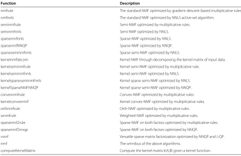
Table 1 Algorithms of NMF variants
Function Description
nmfrule The standard NMF optimized by gradient-descent-based multiplicative rules.
nmfnnls The standard NMF optimized by NNLS active-set algorithm.
seminmfrule Semi-NMF optimized by multiplicative rules.
seminmfnnls Semi-NMF optimized by NNLS.
sparsenmfnnls Sparse-NMF optimized by NNLS.
sparsenmfNNQP Sparse-NMF optimized by NNQP.
sparseseminmfnnls Sparse semi-NMF optimized by NNLS.
kernelnmfdecom Kernel NMF through decomposing the kernel matrix of input data.
kernelseminmfrule Kernel semi-NMF optimized by multiplicative rule.
kernelseminmfnnls Kernel semi-NMF optimized by NNLS.
kernelsparseseminmfnnls Kernel sparse semi-NMF optimized by NNLS.
kernelSparseNMFNNQP Kernel sparse semi-NMF optimized by NNQP.
convexnmfrule Convex-NMF optimized by multiplicative rules.
kernelconvexnmf Kernel convex-NMF optimized by multiplicative rules.
orthnmfrule Orth-NMF optimized by multiplicative rules.
wnmfrule Weighted-NMF optimized by multiplicative rules.
sparsenmf2rule Sparse-NMF on both factors optimized by multiplicative rules.
sparsenmf2nnqp Sparse-NMF on both factors optimized by NNQP.
vsmf Versatile sparse matrix factorization optimized by NNQP andl1QP.
nmf The omnibus of the above algorithms.
computeKernelMatrix Compute the kernel matrix k(A,B) given a kernel function.
A is thus abasis vector. The interpretation is that each data point is a (sparse) non-negative linear combination of the basis vectors. It is well-known that the optimization objective is a non-convex optimization problem, and thus, block-coordinate descentis the main prescribed optimiza-tion technique for such problem. Multiplicative update rules were introduced in [14] for solving Equation (2). Though simple to implement, this algorithm is not guar-anteed to converge to a stationary point [15]. Essentially the optimizations above, with respect toAandY, are non-negative least squares(NNLS). Therefore we implemented the alternating NNLS algorithm proposed in [15]. It can be proven that this algorithm converges to a stationary point. In our toolbox, functionsnmfruleandnmfnnlsare the implementations of the two algorithms above.
Semi-NMF
The standard NMF only works for non-negative data, which limits its applications. Ref. [16] extended it to s emi-NMFwhich removes the non-negative constraints on the data X and basis matrix A. It can be expressed in the following equation:
min A,Y
1
2X−AY 2
F, subject toY≥0. (3)
Semi-NMF can be applied to the matrix of mixed signs, therefore it expands NMF to many fields. How-ever, the gradient-descent-based update rule proposed in [16] is slow to converge (implemented in function seminmfrulein our toolbox). KeepingY fixed, updat-ingAis a least squares problem which has an analytical solution
A=XYT(Y YT)−1=XY†, (4)
where Y† = YT(Y YT)−1 is Moore-Penrose pseudoin-verse. Updating Y while fixing A is a NNLS problem essentially as above. Therefore we implemented the fast NNLS based algorithm to optimize semi-NMF in function seminmfnnls.
Sparse-NMF
solu-tions and also and enhance interpretability of the NMF results. Thesparse-NMF proposed in [3] is expressed in the following equation
min A,Y
1
2X−AY 2 F+
η 2A
2 F+ λ 2 n
i=1
yi21 (5)
subject toA,Y ≥0,
where, yi is the i-th column of Y. From the Bayesian perspective, this formulation is obtained from the log-posterior probability under the assumptions of Gaussian error, Gaussian-distributed basis vectors, and Laplace-distributed coefficient vectors. Keeping one matrix fixed and updating the other matrix can be formulated as a NNLS problem. In order to improve the interpretabil-ity of the basis vectors and speed up the algorithm, we implemented the following model instead:
min A,Y
1
2X−AY 2 F+λ
n
i=1
yi1 (6)
subject toA,Y ≥0,
ai22=1, i=1,· · ·,k.
We optimize this using three alternating steps in each iteration. First, we optimize the following task:
min Y
1
2X−AY 2 F+λ
n
i=1
yi1 (7)
subject toY ≥0.
then,Ais updated as follows:
min A
1
2X−AY 2
F (8)
subject toA≥0.
and then, the columns ofAare normalized to have unitl2 norm. The first and second steps can be solved using non-negative quadratic programming(NNQP), whose general formulation is
min Z
n
i=1 1 2z
T
iHzi+gTi zi+ci (9)
subject toZ≥0,
where,ziis thei-th column of the variable matrixZ. It is easy to prove that NNLS is a special case of NNQP. For example, Equation (7) can be rewritten as
min Y
n
i=1 1 2y
T
i(ATA)yi+(λ−ATxi)Tyi+xTi xi
(10)
subject toY ≥0.
The implementations of the method in [3] and our method are given in functions sparsenmfnnls and
sparseNMFNNQP, respectively. We also implemented the sparse semi-NMF in functionlsparseseminmfnnls.
Versatile sparse matrix factorization
When the training data X is of mixed signs, the basis matrix A is not necessarily constrained to be non-negative; this depends on the application or the inten-tions of the users. However, without non-negativity, A
is not sparse any more. In order to obtain sparse basis matrixAfor some analysis, we may usel1-norm onAto induce sparsity. The drawback of l1-norm is that corre-lated variables may not be simultaneously non-zero in the l1-induced sparse result. This is becausel1-norm is able to produce sparse but non-smooth results. It is known that l2-norm is able to obtain smooth but non-sparse results. When both norms are used together, then corre-lated variables can be selected or removed simultaneously [18]. When smoothness is required on Y, we may also usel2-norm on it in some scenarios. We thus generalize the aforementioned NMF models into a versatile form as expressed below
min
A,Yf(A,Y)= 1
2X−AY 2
F+ k
i=1 (α2
2 ai 2 2
+α1ai1)+
n
i=1 (λ2
2yi 2
2+λ1yi1) (11)
subject to
A≥0 i.e., ift1=1
Y ≥0 i.e., ift2=1 ,
where, parameters: α1 ≥ 0 controls the sparsity of the basis vectors; α2 ≥ 0 controls the smoothness and the scale of the basis vectors;λ1 ≥ 0 controls the sparsity of the coefficient vectors; λ2 ≥ 0 controls the smoothness of the coefficient vectors; and, parameters t1 andt2 are boolean variables (0: false, 1: true) which indicate if non-negativity needs to be enforced onAor Y, respectively. We can call this model versatile sparse matrix factor-ization (VSMF). It can be easily seen that the standard NMF, semi-NMF, and the sparse-NMFs are special cases of VSMF.
We devise the following multiplicative update rules for the VSMF model in the case oft1=t2=1 (implemented in functionsparsenmf2rule):
⎧ ⎨ ⎩
A=A∗ XYT
AY YT+α2A+α1
Y =Y∗ ATX
ATAY+λ2Y+λ1
, (12)
for VSMF (implemented in function vsmf). When t1(ort2) = 1,A (or Y) can be updated by NNQP (this case is also implemented insparsenmf2nnqp). When t1(ort2)=0,A(orY) can be updated using 11QP.
Kernel-NMF
Two features of a kernel approach are that i) it can rep-resent complex patterns, and ii) the optimization of the model is dimension-free. We now show that NMF can also be kernelized.
The basis matrix is dependent on the dimension of the data, and it is difficult to represent it in a very high (even infinite) dimensional space. We notice that in the NNLS optimization, updatingY in Equation (10) needs only the inner products ATA, ATX, and XTX. From Equation (4), we obtain ATA = (Y†)TXTXY†, ATX =
(Y†)TXTX. Therefore, we can see that only the inner product XTX is needed in the optimization of NMF. Hence, we can obtain the kernel version,kernel-NMF, by replacing the inner product XTX with a kernel matrix K(X,X). Interested readers can refer to our recent paper [6] for further details. Based on the above derivations, we implemented the kernel semi-NMF using multiplica-tive update rule (inkernelseminmfrule) and NNLS (in kernelseminmfnnls). The sparse kernel semi-NMFs are implemented in functions kernelsparse-seminmfnnls and kernelSparseNMFNNQP which are equivalent to each other. The kernel method of decom-posing a kernel matrix proposed in [19] is implemented in kernelnmfdecom.
Other variants
Ref. [16] proposed the Convex-NMF, in which the columns of A are constrained to be the convex combi-nations of data points in X. It is formulated as X± =
X±W+Y+ + E, where M± indicates that matrix M is
of mixed signs. XW = A and each column of W
contains the convex coefficients of all the data points to get the corresponding column of A. It has been demonstrated that the columns of A obtained with the convex-NMF are close to the real centroids of clus-ters. Convex-NMF can be kernelized as well [16]. We implemented the convex-NMF and its kernel version inconvexnmfrule andkernelconvexnmf, respec-tively.
The basis vectors obtained with the above NMFs are non-orthogonal. Alternatively, orthogonal NMF (ortho-NMF) imposes the orthogonality constraint in order to enhance sparsity [20]. Its formulation is
X=ASY+E (13)
subject toATA=I, Y YT=I, A,S,Y ≥0,
where, the input X is non-negative,Sabsorbs the mag-nitude due to the normalization of A and Y. Func-tion orthnmfrule is its implementation in our tool-box. Ortho-NMF is very similar with the non-negative sparse PCA (NSPCA) proposed in [21]. The disjoint property on ortho-NMF may be too restrictive for many applications, therefore this property is relaxed in NSPCA. Ortho-NMF does not guarantee the maximum-variance property which is also relaxed in NSPCA. However NSPCA only enforces non-negativity on the basis vectors, even when the training data have neg-ative values. We plan to devise a model in which the disjoint property, the maximum-variance prop-erty, the non-negativity and sparsity constraints can be controlled on both basis vectors and coefficient vec-tors.
There are two efficient ways of applying NMF on data containing missing values. First, the missing values can be estimated prior to running NMF. Alternatively, weighted-NMF [22] can be directly applied to decom-pose the data. Weighted-NMF puts a zero weight on the missing elements and hence only the non-missing data contribute to the final result. An expectation-maximization (EM) based missing value estimation dur-ing the execution of NMF may not be efficient. The weighted-NMF is given in our toolbox in function wnmfrule.
Results and discussion
Based on the various implemented NMFs, a number of data mining tasks can be performed via our toolbox. Table 2 lists the data mining functionalities we provide in this level. These mining tasks are also described along with appropriate examples.
Clustering and bi-clustering
NMF has been applied for clustering. Given dataXwith multivariate data points in the columns, the idea is that, after applying NMF onX, a multivariate data point, say
xiis a non-negative linear combination of the columns of
A; that is xi ≈ Ayi = y1ia1+ · · · +ykiak. The largest coefficient in the i-th column of Y indicates the clus-ter this data point belongs to. The reason is that if the data points are mainly composed with the same basis vec-tors, they should therefore be in the same group. A basis vector is usually viewed as a cluster centroid or proto-type. This approach has been used in [2] for clustering microarray data and in order to discover tumor subtypes. We implemented functionNMFClusterthrough which various NMF algorithms can be selected. An example is provided in exampleCluster file in the folder of our toolbox.
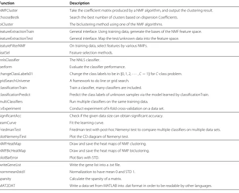
Table 2 NMF-based data mining approaches
Function Description
NMFCluster Take the coefficient matrix produced by a NMF algorithm, and output the clustering result.
chooseBestk Search the best number of clusters based on dispersion Coefficients.
biCluster The biclustering method using one of the NMF algorithms.
featureExtractionTrain General interface. Using training data, generate the bases of the NMF feature space.
featureExtractionTest General interface. Map the test/unknown data into the feature space.
featureFilterNMF On training data, select features by various NMFs.
featSel Feature selection methods.
nnlsClassifier The NNLS classifier.
perform Evaluate the classifier performance.
changeClassLabels01 Change the class labels to be in{0, 1, 2,· · ·,C−1}forC-class problem.
gridSearchUniverse A framework to do line or grid search.
classificationTrain Train a classifier, many classifiers are included.
classificationPredict Predict the class labels of unknown samples via the model learned by classificationTrain.
multiClassifiers Run multiple classifiers on the same training data.
cvExperiment Conduct experiment of k-fold cross-validation on a data set.
significantAcc Check if the given data size can obtain significant accuracy.
learnCurve Fit the learning curve.
FriedmanTest Friedman test with post-hoc Nemenyi test to compare multiple classifiers on multiple data sets.
plotNemenyiTest Plot the CD diagram of Nemenyi test.
NMFHeatMap Draw and save the heat maps of NMF clustering.
NMFBicHeatMap Draw and save the heat maps of NMF biclustering.
plotBarError Plot Bars with STD.
writeGeneList Write the gene list into a .txt file.
normmean0std1 Normalization to have mean 0 and STD 1.
sparsity Calculate the sparsity of a matrix.
MAT2DAT Write a data set from MATLAB into .dat format in order to be readable by other languages.
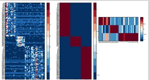
rows and columns of matrixX. This is bi-clustering and the interested readers can refer to [23] for an excellent survey on clustering algorithms and to [4] for a bi-clustering method based on NMF. We implemented a bi-clustering approach based on NMF in biCluster function. The bi-clusters can be visualized via the function NMFBicHeatMap. We applied NMF to simultaneously grouping the genes and samples of a leukemia data set [2] which includes tumor samples of three subtypes. The goal is to find strongly correlated genes over a subset of samples. A subset of such genes and a subset of such sam-ples form a bi-cluster. The heat-map is shown in Figure 1. Readers can find the script inexampleBiClusterfile of our toolbox.
Basis vector analysis for biological process discovery We can obtain interesting and detailed interpretations via an appropriate analysis of the basis vectors. When applying NMF on a microarray data, the basis vectors
are interpreted as potential biological processes [3,13,24]. In the following, we give one example for finding bio-logical factors on gene-sample data, and two examples on time-series data. Please note they only serve as sim-ple examsim-ples. Fine tuning of the parameters of NMF is necessary for accurate results.
First example
28 30 31 32 33 34 35 36 37 38 10 20 21 22 23 24 25 26 27 1 2 3 4 5 6 7 8 9 11 12 13 14 15 16 17 18 19 29 4701 4679 4495 4243 4111 3984 3948 3867 3662 3634 3308 3281 3277 3270 3208 3160 2994 2990 2654 2604 2429 2421 2365 2197 1930 1787 1668 1666 1618 1488 1374 1244
1218 941
885 873 626 322 190 91 39 2 4831 4794 4531 4286 4264 4018 3291 3035 2310 2308 2256 2224 1260 4870 4828 4812 4809 4516 4458 4454 4120 4017 4003 3987 3960 3930 3640 3584 3474 3400 3346 3271 3126 3082 3060 3051 3000 2961 2936 2926 2882 2339 2072 2010 1555 1412 1386 1338 1274
1137 802
731 254 214 202 94
1 2 3
4701 4679 4495 4243 4111 3984 3948 3867 3662 3634 3308 3281 3277 3270 3208 3160 2994 2990 2654 2604 2429 2421 2365 2197 1930 1787 1668 1666 1618 1488 1374 1244
1218 941
885 873 626 322 190 91 39 2 4831 4794 4531 4286 4264 4018 3291 3035 2310 2308 2256 2224 1260 4870 4828 4812 4809 4516 4458 4454 4120 4017 4003 3987 3960 3930 3640 3584 3474 3400 3346 3271 3126 3082 3060 3051 3000 2961 2936 2926 2882 2339 2072 2010 1555 1412 1386 1338 1274
1137 802
731 254 214 202 94
28 30 31 32 33 34 35 36 37 38 10 20 21 22 23 24 25 26 27 1 2 3 4 5 6 7 8 9 11 12 13 14 15 16 17 18 19 29
3 2 1 −1 −0.5 0 0.5 1 −0.5 0 0.5 1 0 1 2 3 4 5
Figure 1Heat map of NMF biclustering result.Left: the gene expression data where each column corresponds to a sample. Center: the basis matrix. Right: the coefficient matrix.
tools, such as MIPS [26], GOTermFinder [27], and DAVID [28,29].
Second example
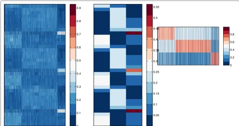
We used NMF to cluster a time-series data of yeast metabolic cycle in [30]. Figure 2 shows the heat-map of NMF clustering, and Figure 3 shows the three basis vec-tors. We usednmfnnlsfunction to decompose the data and NMFHeatMap to plot the heat-map. The detailed script is given in the exampleBioProcessTSYeast file in the toolbox. We can clearly see that the three peri-odical biological processes corresponds exactly to the Ox (oxidative), R/B (reductive, building), and R/C (reductive, charging) processes discovered in [30].
Third example
We used NMF to factorize a breast cancer time-series data set, which includes wild type MYCN cell lines and mutant MYCN cell lines [31]. The purpose of this exam-ple is to show that NMF is a potential tool to finding cancer drivers. One basic methodology is in the follow-ing. First, basis vectors are produced applying NMF on a time-series data. Then factor-specific genes are identified by computational or statistical methods. Finally, the reg-ulators of these factor-specific genes are identified from any prior biological knowledge. This data set has 8 time points (0, 2, 4, 8, 12, 24, 36, 48 hr.). The zero time point is untreated and samples were collected at the subsequent
time points after treatment with 4-hydroxytamoxifen (4-OHT). In our computational experiment, we use our VSMF implementation (functionvsmf). We set k = 2. Because this data set has negative values we sett1 = 0 andt2 = 1. We setα1 = 0.01,α2 = 0,λ1 = 0, and λ2 = 0.01. The basis vectors of both wild-type and mutant data are compared in Figure 4. From the wild-type time-series data, we can successfully identify two patterns. The rising pattern corresponds to the induced signature and the falling pattern corresponding to the repressed signature in [31]. It is reported in [31] that the MYC target genes contributes to both patterns. From the mutant time-series, we can obtain two flat pro-cesses, which are reasonable. The source code of this example can be found in exampleBioProcessMYC. We also recommend the readers to see the meth-ods based on matrix decompositions which are proposed in [13,32] and devised for identifying signaling pathways.
Basis vector analysis for gene selection
Table 3 Gene set enrichment analysis using Onto-Express for the factor specific genes identified by NMF
Factor 1 Factor 2 Factor 3
biological process p-value biological process p-value biological process p-value
reproduction (5) 0 response to stimulus (15) 0.035 regulation of bio. proc. (226) 0.009
metabolic process (41) 0 biological regulation (14) 0.048 multi-organism proc. (39) 0.005
cellular process (58) 0 biological regulation (237) 0.026
death (5) 0
developmental process (19) 0
regulation of biological process (19) 0
idea is to conduct gene selection on the metasamples. The reason is that the discovered biological processes via NMF are biologically meaningful for class discrim-ination in disease prediction, and the genes expressed differentially across these processes contribute to bet-ter classification performance in bet-terms of accuracy. In Figure 1 for example, three biological processes are discovered and only the selected genes are shown. We have implemented the information-entropy-based gene selection approach proposed in [3] in function featureFilterNMF. We give an example on how to call this function in fileexampleFeatureSelection. It has been reported that it can select meaningful genes, which has been verified with gene ontology analysis. Fea-ture selection based on supervised NMF will also be implemented.
Feature extraction
Microarray data and mass spectrometry data have tens of thousands of features but only tens or hundreds of samples. This leads to the issues of curse of dimen-sionality. For example, it is impossible to estimate the parameters of some statistical models since the number of their parameters grow exponentially as the dimension increases. Another issue is that biological data are usually noisy; which crucially affects the performances of clas-sifiers applied on the data. In cancer study, a common hypothesis is that only a few biological factors (such as the oncogenes) play a crucial role in the development of a given cancer. When we generate data from control and sick patients, the high-dimensional data will contain a large number of irrelevant or redundant information. Orthogonal factors obtained with principal component
0 0.2 0.4 0.6 0.8
0.05 0.1 0.15 0.2 0.25 0.3 0.35 0.4 0.45 0.5 0.55
0 0.1 0.2 0.3 0.4 0.5 0.6 0.7 0.8 0.9
5 10 15 20 25 30 35 0
0.1 0.2 0.3 0.4 0.5 0.6 0.7
Time Point
Intensity
cluster 1 cluster 2 cluster 3
Figure 3Biological processes discovered by NMF on yeast metabolic cycle time-series data.
0 5 10 15 20 25 30 35 40 45
−0.8 −0.6 −0.4 −0.2 0 0.2 0.4 0.6
Time Point
Gene Expression Level
Rising(Wide−Type) Falling(Wide−Type) Flat(Mutant) Flat(Mutant)
analysis(PCA) orindependent component analysis(ICA) are not appropriate in most cases. Since NMF generates non-orthogonal (and non-negative) factors, therefore it is much reasonable to extract important and interesting fea-tures from such data using NMF. As mentioned above, training dataXm×n, withmfeatures andnsamples, can be decomposed intokmetasamplesAm×kandYk×n, that is
X≈AYtr, subject toA,Ytr≥0, (14)
where, Ytr means that Y is obtained from the training data. The k columns of A span the k-dimensional fea-ture spaceand each column ofYtr is the representation of the corresponding original training sample in the fea-ture space. In order to project the punknown samples
Sm×pinto this feature space, we have to solve the following non-negative least squares problem:
S≈AYuk, subject toYuk≥0, (15)
where,Yukmeans the Y is obtained from the unknown samples. After obtaining Ytr andYuk, the learning and prediction steps can be done quickly in thek-dimensional feature space instead of them-dimensional original space. A classifier can learn overYtr, and then predicts the class
labels of the representations of unknown samples, that is
Yuk.
From the aspect of interpretation, the advantage of NMF over PCA and ICA is that the metasamples are very useful in the understanding of the underlying biological processes, as mentioned above.
We have implemented a pair of functions feature-ExtractionTrain and featureExtractionTest including many linear and kernel NMF algorithms. The basis matrix (or, the inner product of basis matrices in the kernel case) is learned from the training data via
the function featureExtractionTrain, and the
unknown samples can be projected onto the feature space via the function featureExtractionTest.
We give examples of how to use these
func-tions in files exampleFeatureExtraction and
exampleFeatureExtractionKernel.
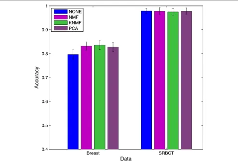
Figure 5 shows the classification performance of SVM without dimension reduction and SVM with dimension reduction using linear NMF, kernel NMF with radial basis function (RBF) kernel, and PCA on two data sets, SRBCT [33] and Breast [34]. Since ICA is computation-ally costly, we did not include it in the comparisons.
Breast SRBCT
0.4 0.5 0.6 0.7 0.8 0.9 1
Data
Accuracy
NONE NMF KNMF PCA
The bars represent the averaged 4-fold cross-validation accuracies usingsupport vector machine (SVM) as clas-sifier over 20 runs. We can see that NMF is compara-ble to PCA on SRBCT, and is slightly better than PCA on Breast data. Also, with only few factors, the perfor-mance after dimension reduction using NMF is at least comparable to that without using any dimension reduc-tion. As future work, supervised NMF will be investi-gated and implemented in order to extract discriminative features.
Classification
If we make the assumption that every unknown sam-ple is a sparse non-negative linear combination of the training samples, then we can directly derive a classi-fier from NMF. Indeed, this is a specific case of NMF in which the training samples are the basis vectors. Since the optimization process within NMF is a NNLS problem, we call this classification approach the NNLS classifier [35]. A NNLS problem is essentially a quadratic program-ming problem as formulated in Equation (9), therefore, only inner products are needed for the optimization. We thus can naturally extend the NNLS classifier to kernel
version. Two features of this approach are that: i) the spar-sity regularization help avoid overfitting the model; and ii) the kernelization allows a dimension-free optimiza-tion and also linearizes the non-linear complex patterns within the data. The implementation of the NNLS classi-fier is in filennlsClassifier. Our toolbox also pro-vides many other classification approaches including SVM classifier. Please see file exampleClassification for demonstration. In our experiment of 4-fold cross-validation, accuracies of 0.7865 and 0.7804 are respec-tively obtained with linear and kernel (RBF) NNLS classifier on Breast data set. They achieved accura-cies of 0.9762 and 0.9785, respectively, over SRBCT data.
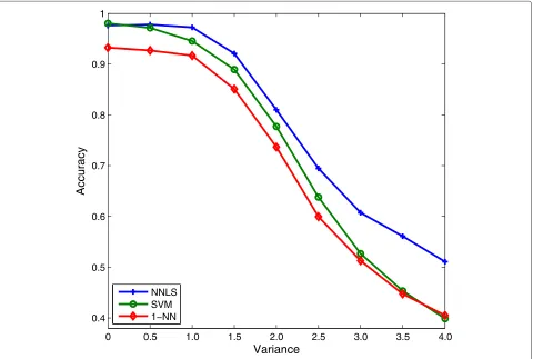
Biological data are usually noisy and sometimes contain missing values. A strength of the NNLS classifier are that it is robust to noise and to missing values, making NNLS classifiers quite suitable for classifying biological data [35]. In order to show its robustness to noise, we added a Gaussian noise of mean 0 and variance from 0 to 4 with increment 0.5 on SRBCT. Figure 6 illustrates the results of NNLS, SVM, and 1-nearest neighbor (1-NN) classifiers using this noisy data. It can be seen that as
0 0.5 1.0 1.5 2.0 2.5 3.0 3.5 4.0
0.4 0.5 0.6 0.7 0.8 0.9 1
Variance
Accuracy
NNLS SVM 1−NN
the noise increases, NNLS outperforms SVM and 1-NN significantly.
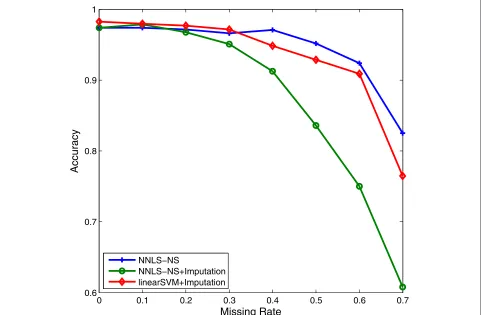
To deal with the missing value problem, three strategies are usually used: incomplete sample or feature removal, missing value imputation (i.e., estimation), and ignoring missing values. Removal methods may delete important or useful information for classification and particularly when there is a large percentage of missing values in the data. Imputation methods may create false data depend-ing on the magnitude of the true estimation errors. The third method ignores using the missing values during clas-sification. Our approach in dealing with the missing value problem is also to ignore them. The NNLS optimization needs only the inner products of pairs of samples. Thus, when computing the inner product of two samples, sayxi andxj, we normalize them to have unitl2-norm using only the features present in both samples, and then we take their inner product. As an example, we randomly removed between 10% to 70% of data values in STBCT data. Using such incomplete data, we compared our method with the zero-imputation method (that is, estimating all missing values as 0). In Figure 7, we can see that the NNLS
clas-sifier using our missing value approach outperforms the zero-imputation method in the case of large missing rate. Also, the more sophisticatedk-nearest neighbor imputa-tion (KNNimpute) method [36] will fail on data with in high percentage of missing values.
Statistical comparison
The toolbox provides two methods for statistical compar-isons and evaluations of different methods. The first is a two-stage method proposed in [37]. The importance of this method is that it can estimate the data-size require-ment for attaining a significant accuracy and extrapolate the performance based on the current available data. Generating biological data is usually very expensive and thus this method can help researchers to evaluate the necessity of producing more data. At the first stage, the minimum data size required for obtaining a sig-nificant accuracy is estimated. This is implemented in function significantAcc. The second stage is to fit the learning curve using the error rates of large data sizes. It is implemented in functionlearnCurve. In our experiments, we found that the NNLS classifier usually
0 0.1 0.2 0.3 0.4 0.5 0.6 0.7
0.6 0.7 0.8 0.9 1
Missing Rate
Accuracy
NNLS−NS
NNLS−NS+Imputation linearSVM+Imputation
0 20 40 60 80 100 120 140 160 180 200 0
0.05 0.1 0.15 0.2 0.25
Sample Size
Error Rate
NNLS Average NNLS 25% Quantile NNLS 75 Quantitle SVM Mean SVM 25% Quantitle SVM 75% Quantitle
Figure 8The fitted learning curves of NNLS and SVM classifiers on SRBCT data.
requires fewer number of samples for obtaining a sig-nificant accuracy. For example on SRBCT data, NNLS requires only 4 training samples while SVM needs 19 training samples. The fitted learning curves of NNLS and SVM classifiers are shown in Figure 8. We pro-vide an example of how to plot this figure in file exampleFitLearnCurve.
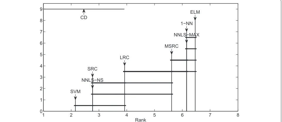
The second method is the nonparametric Friedman test coupled with post-hoc Nemenyi test to compare multiple classifiers over multiple data sets [38]. It is diffi-cult to draw an overall conclusion if we compare multiple approaches in a pairwise fashion. Friedman test has been recommended in [38] because it is simple, safe and robust, compared with parametric tests. It is implemented in
1 2 3 4 5 6 7 8
0 1 2 3 4 5 6 7 8 9
Rank SVM
NNLS−NS SRC
LRC
MSRC
NNLS−MAX 1−NN
ELM CD
function FriedmanTest. The result can be presented graphically using the crucial difference(CD) diagram as implemented in function plotNemenyiTest. CD is determined by significant levelα. Figure 9 is an example of the result of the Nemenyi test for comparing 8 classifiers over 13 high dimensional biological data sets. This exam-ple can be found in fileexampleFriedmanTest. If the distance of two methods is greater than the CD then we conclude that they differ significantly.
Conclusions
In order to address the issues of the existing NMF imple-mentations, we propose a NMF Toolbox written in MAT-LAB, which includes a basic NMF optimization level and an advanced data mining level. It enable users to analyze biological data via NMF-based data mining approaches, such as clustering, bi-clustering, feature extraction, fea-ture selection, and classification .
The following are the future works planned in order to improve and augment the toolbox. First, we will include more NMF algorithms such as nsNMF, LS-NMF, and supervised NMF. Second, we are very interested in imple-menting and speeding up the Bayesian decomposition method which is actually a probabilistic NMF intro-duced independently in the same period as the standard NMF. Third, we will include more statistical comparison and evaluation methods. Furthermore, we will investi-gate the performance of NMF for denoising and for data compression.
Availability and requirements
Project name:The NMF Toolbox in MATLAB
Project home page: https://sites.google.com/site/ nmftool and http://cs.uwindsor.ca/~li11112c/nmf Operating system(s):Platform independent
Programming language:MATLAB
Other requirements:MATLAB 7.11 or higher License:GNU GPL Version 3
Any restrictions to use by non-academics: Licence needed
Competing interests
The authors declare that they have no competing interests.
Authors’ contributions
YL did comprehensive survey on NMF, implemented the toolbox, and drafted this manuscript. AN supervised the whole project, provided constructive suggestions on this toolbox, and wrote the final manuscript. All authors read and approved the final manuscript.
Acknowledgements
This research has been partially supported by IEEE CIS Walter Karplus Summer Research Grant 2010, Ontario Graduate Scholarship 2011–2013, and Canadian NSERC Grants #RGPIN228117–2011.
Received: 30 November 2012 Accepted: 10 April 2013 Published: 16 April 2013
References
1. Lee DD, Seung S:Learning the parts of objects by non-negative matrix factorization.Nature1999,401:788–791.
2. Brunet J, Tamayo P, Golub T, Mesirov J:Metagenes and molecular pattern discovery using matrix factorization.PNAS2004, 101(12):4164–4169.
3. Kim H, Park H:Sparse non-negatice matrix factorization via alternating non-negativity-constrained least aquares for microarray data analysis.SIAM J Matrix Anal Appl2007,23(12):1495–1502. 4. Carmona-Saez P, Marqui RD, Tirado F, Carazo JM,
Pascual-Montano A:Biclustering of gene expression data by non-smooth non-negative matrix factorization.BMC Bioinformatics2006,7:78. 5. Wang G, Kossenkov A, Ochs M:LS-NMF: A modified non-negative matrix factorization algorithm utilizing uncertainty estimates. BMC Bioinformatics2006,7:175.
6. Li Y, Ngom A:A new kernel non-negative matrix factorization and its application in microarray data analysis.InCIBCB: IEEE CIS Society Piscataway: IEEE Press; 2012:371–378.
7. Cichocki A, Zdunek R:NMFLAB - MATLAB toolbox for non-negative matrix factorization.Tech. rep. 2006, [http://www.bsp.brain.riken.jp/ ICALAB/nmflab.html]
8. The NMF: DTU toolbox.Tech. rep., Technical University of Denmark, [http://cogsys.imm.dtu.dk/toolbox/nmf]
9. Liu S:NMFN: non-negative matrix factorization.Tech. rep., Duke University, 2011, [http://cran.r-project.org/web/packages/NMFN] 10. Gaujoux R, Seoighe C:A flexible R package for nonnegative matrix
factorization.BMC Bioinformatics2010,11:367. [http://cran.r-project. org/web/packages/NMF]
11. Qi Q, Zhao Y, Li M, Simon R:non-negative matrix factorization of gene expression profiles: A plug-in for BRB-ArrayTools.Bioinformatics2009, 25(4):545–547.
12. Fertig E, Ding J, Favorov A, Parmigiani G, Ochs M:CoGAPS: an R/C++ package to identify patterns and biological process activity in transcriptomic data.Bioinformatics2010,26(21):2792–2793. 13. Ochs M, Fertig E:Matrix factorization for transcriptional regulatory
network inference.InCIBCB, IEEE CIS Society. Piscataway: IEEE Press; 2012:387–396.
14. Lee D, Seung S:Algorithms for non-negative matrix factorization. InNIPS: Cambridge: MIT Press; 2001:556–562.
15. Kim H, Park H:Nonnegative matrix factorization based on alternating nonnegativity constrained least squares and active set method. SIAM J Matrix Anal Appl2008,30(2):713–730.
16. Ding C, Li T, Jordan MI:Convex and semi-nonnegative matrix factorizations.TPAMI2010,32:45–55.
17. Tibshirani R:Regression shrinkage and selection via the lasso.J R Stat Soc Ser B (Methodol)1996,58:267–288.
18. Zou H, Hastie T:Regularization and variable selection via the elastic Net.J R Stat Soc- Ser B: Stat Methodol2005,67(2):301–320.
19. Zhang D, Zhou Z, Chen S:Non-negative matrix factorization on kernels.LNCS2006,4099:404–412.
20. Ding C, Li T, Peng W, Park H:Orthogonal nonnegative matrix tri-factorizations for clustering.InKDD. New York: ACM; 2006:126–135. 21. Zass R, Shashua A:Non-negative sparse PCA.InNIPS. Cambridge: MIT
Press; 2006.
22. Ho N:Nonnegative matrix factorization algorithms and applications. PhD thesis. Louvain-la-Neuve: Belgium; 2008.
23. Madeira S, Oliveira A:Biclustering algorithms for biological data analysis: A survey.IEEE/ACM Trans Comput Biol Bioinformatics2004, 1:24–45.
24. Kim P, Tidor B:Subsystem identification through dimensionality reduction of large-scale gene expression data.Genome Res2003, 13:1706–1718.
25. Draghici S, Khatri P, Bhavsar P, Shah A, Krawetz S, Tainsky M:Onto-tools, the toolkit of the modern biologist: onto-express, onto-compare, onto-design and onto-translate.Nucleic Acids Res2003,
31(13):3775–3781.
26. Mewes H, Frishman D, Gruber C, Geier B, Haase D, Kaps A, Lemcke K, Mannhaupt G, Pfeiffer F, Schuller C, Stocker S, Weil B:MIPS: A database for genomes and protein sequences.Nucleic Acids Res2000,28:37–40. 27. Boyle E, Weng S, Gollub J, Jin H, Botstein D, Cherry J, Sherlock G:
information and finding significantly enriched gene ontology terms associated with a list of genes.Bioinformatics2004,20:3710–3715. 28. Huang D, Sherman B, Lempicki R:Systematic and integrative analysis
of large gene lists using DAVID Bioinformatics resources.Nature Protoc2009,4:44–57.
29. Huang D, Sherman B, Lempicki R:Bioinformatics enrichment tools: paths toward the comprehensive functional analysis of large gene lists.Nucleic Acids Res2009,37:1–13.
30. Tu B, Kudlicki A, Rowicka M, McKnight S:Logic of the yeast metabolic cycle: temporal compartmentalization of cellular processes.Science 2005,310:1152–1158.
31. Chandriani S, Frengen E, Cowling V, Pendergrass S, Perou C, Whitfield M, Cole M:A core MYC gene expression signature is prominient in basal-like breast cancer but only partially overlaps the core serum response.PloS ONE2009,4(5):e6693.
32. Ochs M, Rink L, Tarn C, Mburu S, Taguchi T, Eisenberg B, Godwin A: Detection of treatment-induced changes in signaling pathways in sastrointestinal stromal tumors using transcripttomic data.Cancer Res2009,69(23):9125–9132.
33. Khan J:Classification and diagnostic prediction of cancers using gene expression profiling and artificial neural networks.Nat Med 2001,7(6):673–679.
34. Hu Z:The molecular portraits of breast tumors are conserved across microarray platforms.BMC Genomics2006,7:96.
35. Li Y, Ngom A:Classification approach based on non-negative least squares.Neurocomputing2013, in press.
36. Troyanskaya O, Cantor M, Sherlock G, Brown P, Hastie T, Tibshirani R, Botstein D, Altman R:Missing value estimation methods for DNA microarrays.Bioinformatics2001,17(6):520–525.
37. Mukherjee S, Tamayo P, Rogers S, Rifkin R, Engle A, Campbell C, Golub T, Mesirov J:Estimating dataset size requirements for classifying DNA microarray data.J Comput Biol2003,10(2):119–142.
38. Demsar J:Statistical comparisons of classifiers over multiple data sets.J Mach Learn Res2006,7:1–30.
doi:10.1186/1751-0473-8-10
Cite this article as:Li and Ngom:The non-negative matrix factorization toolbox for biological data mining.Source Code for Biology and Medicine2013
8:10.
Submit your next manuscript to BioMed Central and take full advantage of:
• Convenient online submission
• Thorough peer review
• No space constraints or color figure charges
• Immediate publication on acceptance
• Inclusion in PubMed, CAS, Scopus and Google Scholar
• Research which is freely available for redistribution