A generalization of Profile Hidden Markov Model (PHMM) using one-by-one dependency between sequences

(1)

Progress in Biological Sciences / Vol. 6 (2) 2016

A generalization of Profile Hidden Markov Model (PHMM) using one-by-one dependency between sequences ... 117

Vahid Rezaei Tabar, Hamid Pezeshk

Neighborhood matrix: A new idea in matching of two dimensional gel images ... 129

Behrouz Alizadeh Savareh1, Azadeh Bashiri2, Mehrnaz Mostafavi

Optimization for high level expression of cold and pH tolerant amylase in a newly isolated Pedobacter sp. through Response Surface Methodology ... 139

Razie Ghazi-Birjandi, Bahar Shahnavaz, Maryam Mahjoubin-Tehran

Using petrochemical wastewater for production of cruxrhodopsin as an energy capturing nanoparticle by

Haloarcula sp. IRU1 ... 151

Mojtaba Taran, Mehran Alavi, Arina Monazah, Javad Zavar Reza

Radical scavengering of pigments from novel strains of Dietzia schimae and Microbacterium esteraromaticum ... 159

Sayyede Narjes Zamanian, Zahra Etemadifar

Degradation of naphthalene by bacterial isolates from the Gol Gohar Mine, Iran ... 171

Moslem Abarian, Mehdi Hassanshahian, Arastoo Badoei-Dalfard

Evaluation of growth inhibition activity of myxobacterial extracts against multi-drug resistant

Acinetobacter baumannii ... 181

Mona Dehhaghi, Fatemeh Mohammadipanah

Comparison of MAPK and thioredoxin gene expression in wheat seedlings exposed to silver nitrate and silver nanoparticle ... 189

Javad Karimi; Sasan Mohsenzadeh

Simple procedure for production of short DNA size markers of 100 to 2000 bp ... 199

Hamed Hekmatnezhad, Fatemeh Moradian, Seyed Hamidreza Hashemi-Petroudi

Changes in composition and antioxidant activities of essential oils in Phlomis anisodonta (Lamiaceae) at different stages of maturity ... 205

Hamzeh Amiri

Effects of culture medium and supplementation on seed germination, protocorm formation and regeneration of some Phalaenopsis hybrids ... 213

Golandam Sharifi, Masoud Mirmasoumi, Zahra Zahed

Subgeneric classification of Linaria (Plantaginaceae; Antirrhineae): molecular phylogeny and morphology revisited ... 229

Nafiseh Yousefi, Günther Heubl, Shahin Zarre

(2)

(3)

Progress in Biological Sciences

Vol. 6, Number 2, Summer / Autumn 2016/117-127 – DOI: 10.22059/PBS.2016.590014

A generalization of Profile Hidden Markov Model (PHMM)

using one-by-one dependency between sequences

Vahid Rezaei Tabar1,2

*, Hamid Pezeshk2,3

1

Department of Statistics, Faculty of mathematics and Computer Sciences, Allameh Tabataba'i University, Tehran, Iranz

2

School of Computer Science, Institute for Research in Fundamental Science (IPM), Tehran, Iran

3

School of Mathematics, Statistics and Computer Science, University of Tehran, Iran

Received: May 12, 2016; Accepted: December 10, 2016

The Profile Hidden Markov Model (PHMM) can be poor at capturing dependency between observations because of the statistical assumptions it makes. To overcome this limitation, the dependency between residues in a multiple sequence alignment (MSA) which is the representative of a PHMM can be combined with the PHMM. Based on the fact that sequences appearing in the final MSA are written based on their similarity; the one-by-one dependency between corresponding amino acids of two current sequences can be append to PHMM. This perspective makes it possible to consider a generalization of PHMM. For estimating the parameters of generalized PHMM (emission and transition probabilities), we introduce new forward and backward algorithms. The performance of generalized PHMM is discussed by applying it to the twenty protein families in Pfam database. Results show that the generalized PHMM significantly increases the accuracy of ordinary PHMM.

Keywords: Statistics; Multiple sequence alignment; Amino Acids; Protein families; Pfam database

Introduction

A hidden Markov model (HMM) is a statistical Markov model in which the system being modeled is assumed to be a Markov process with unobserved (hidden) states (1, 2, 3). It is used in almost all current speech recognition system, in numerous applications in computational molecular biology, in data com-pression, and in other areas of artificial and pattern recognition (4, 5, 6, 7). A Hidden Markov Model (HMM) can be presented as a specific type of

graphical model which is a directed acyclic graph (DAG) (Figure 1). Under the casual Markov assumption, the joint probability distribution of a HMM can be written as:

( ) ( ) ∏ ( | ) ( | ) {1}

in which ( | ) and ( | )indicate the transition and emission probabilities.

(4)

Figure 1. Structure of a HMM

Sonnhammer et al. (8) introduced an HMM architecture that was well suited for representing profiles of multiple sequence alignments (MSA). For each consensus column of the multiple alignment, a "Match" (M) state models the distribution of residues allowed in the column. An "Insert" (I) state and

"Delete" (D) state at each column allow for insertion one or more residues between that column and the next, or for deleting the consensus residues. Profile HMMs are strongly linear, left-right models. Figure 2 shows a profile HMM corresponding to the MSA.

Figure 2. Structure of a profile HMM

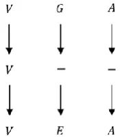
The Profile Hidden Markov Model (PHMM) can be poor at capturing dependency between observations because of the statistical assumptions it makes (1). For overcoming this problem, we consider the one-by-one dependency between two current residues. Based on the fact that with doing a MSA, the sequences are biologically related, we can use the MSA to find the areas of similarity between two current sequences. Therefore the one-by-one dependency between a residue and the corresponding residue located above it can be combined with the PHMM (i.e. Figure 3).

Figure 3. One-by-one dependency between sequences in MSA

This approach in spirit is similar to the works proposed by Holmes (9), Qian and Goldstein (10) and Siepel and Haussler (11) where a PHMM is augmented with phylogenetic trees. In their approach, the evolutionary information is appended to the PHMM. They considered the dependency between sequences based on the fact that all the current sequences are dependent upon their ancestral sequences and there is no dependency between two current sequences. But in our approach, the dependency between two current sequences based on the similarity between them can be appended to the PHMM.

When talking about PHMMs, there are generally three problems to be considered (12):

(5)

Vahid Rezaei Tabar, Hamid Pezeshk

Progress in Biological Sciences / Vol. 6 (2) 2016 / 117-127

119

Recognition: Given the observation sequence O={O_1,O_2,…,O_L} and a model λ, how do we choose a corresponding state sequence S={S_1,S_2,…,S_L} which is optimal in some sense, i.e., best explains the observations. For this problem the Viterbi algorithm is used (13).

Training: Given the observation sequence O={O_1,O_2,…,O_L}, how do we adjust the model parameters λ to maximize P(O|λ). For this purpose the Baum Welch (forward-backward) algorithm is considered (14).

In this paper, based on the one-by-one dependency between two current sequences, we introduce the new forward and backward algorithms. As a result, the Baum-Welch and Viterbi algorithms are generalized.

This paper organizes as follows: in section 2, we introduce the PHMM. In section 3, parameter estimation of PHMM is presented. More details of generalized Viterbi algorithm presented in section 4. We finally compare the performance of the generalized PHMM with the common one by applying them on twenty protein families in Pfam database which is a well-known database of protein families (15).

Materials and Methods

The PHMM

Profile hidden Markov model (PHMM) techniques are among the most powerful methods for protein homology detection (16). One of the advantages of using the PHMMs is that they provide a better method for dealing with gaps found in protein families. A profile HMM is a linear state machine consisting of a series of nodes, each of which corresponds roughly to a position (column) in the alignment from which it was built (17-19). In other words, the PHMM is a linear structure of three states Match (M), Delete (D), and Insert (I). The construction of the PHMM is shown in Figure 2. In PHMM, we need to decide how many states exist in a PHMM. In other words, we should determine the length of the PHMM (i.e., how many match states do we have in a profile?). Here we assume that n is the number of Match states (M) in the PHMM. So, the total number of states is 3n+3.

Delete, Start and End states are silent and they emit

no symbols. One heuristic method to set M, is to include those columns that have amino acids in at least half of the sequences using MSA (2). It should be noted that in each column, we have 20 amino acids or gap in which 20 amino acids are observed from Match and Insert states. A profile HMM has several types of probabilities associated with it. One type is the transition probability; the probability of transitioning from one state to another. There are also emissions probabilities associated with each Match or Insert state, based on the probability of a given residue existing at that position in the alignment.

Parameter Estimation of the Generalized

PHMM

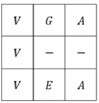
A major limitation of a PHMM is the assumption that given states, the observations, are independent. To overcome this limitation, the dependency between amino acids in a multiple sequence alignment (MSA) which is the representative of a PHMM can be appended to the PHMM. It is very important because we can generalize profile hidden Markov models using the on-by-one dependency. The sequences appearing in the final multiple sequence alignment are written based on their similarity (note that MSA is a representative of PHMM). So, the one-by-one dependency between corresponding amino acids of two current sequences can be combined with PHMM. Regarding MSA, we assume that protein sequences consisting of 21 observations (20 amino acids and one gap) have been placed on a regular lattice. In other words, each observation (residue) is arranged as a site (i.e. Figure 4).

(6)

Regarding the regular lattice, we can introduce the ingredients of the PHMM as follows:

1. Hidden state (S) takes on 3n+3 values

2. Observation (O) takes on 21 values (20 amino acids and gap)

3. Transition probability matrix _{( ) ( )} with following entries:

( ) ( | )

4. Emission probabilities _{( )} with the following entries:

( ) ( | )

.

This emission probability presents the probability of current observed variable given the current hidden state as well as observed variable located above it. It

should be noted that represents the amino acids

(20 types) at lattice point and is the amino acids

or one gap (21 types) located above .

5. A vector of initial state π with elements ( ) ( )

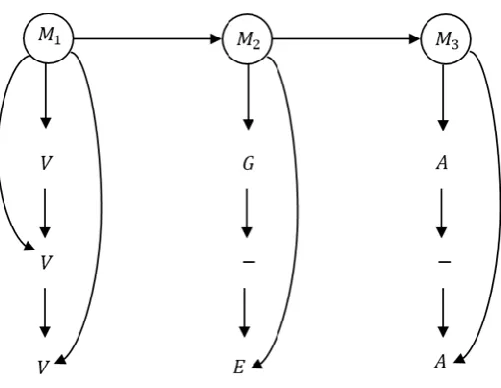
With consideration of the one-by-one dependency between residues, a PHMM can also be considered as a graphical model.

According to Figure 3, if we assume that the observations come from three hidden Match states (M1, M2 and M3), then the dependency between

Match states (from left to right), the dependency between residues (top to bottom), and the dependency between residues and hidden states can be shown in Figure 5.

Figure 5. A PHMM with consideration of the one-by-one dependency

Suppose that

[

]

, where is the

number of rows in MSA (Note that we arrange the observations on the regular lattice). For instance in Figure 4, we have [ ] [ ] [ ].)

Regarding one-by-one dependency between obser-vations, the likelihood of the parameters ( ) given the observations will be as follows:

( | ) ( | ) ∑ ( | ) ( | )

(7)

121

∑ ∏ ( ) ∏ ( ) ( | )

( )

Note that we consider ( ) ( | ) as

the new parameter. In other words, a vector of initial observation φ with elements ( ) ( | ) is added to the set of parameters . Taken together we have ( ). For estimating the set of parameter in a PHMM, we need to define the

new Forward and Backward algorithms which are to find out a recursive way to represent the variable sequence (20).

The Forward algorithm represents the probability of observations up to time t and in state i at time t, given the model λ;

( ) ( | )

Then we have:

( | ) ∑ ( | ) ∑ ( )

We can solve ( ) for inductively through the equation (Note that ):

( ) ( | )

∑ ( | )

∑ ( | ) ( | )

∑ ( ) ( | )

∑ ( ) ( | ) ( | )

∑ ( ) ( ) ( | ) ( | )

( | ) ( | ) ( | )

∑ ( ) ( ) ( | ) ∏ ( | )

∑ ( ) ( ) ( ) ∏ ( )

In a very similar manner, we define the backward variable as follows: ( ) ( | )

(8)

solve ( | ) by the following way:

( ) ( | )

∑ ( | )

∑ ( | ) ( | )

∑ ( | )

( )

∑ ( ) ( | ) ( ) ( | )

( )

∑ ( ) ( ) ( | ) ∏ ( | )

∑ ( ) ( ) ( ) ∏ ( )

Let ( ) be the probability of the PHMM being in state i at time t and making a transition to state j at time

t + 1, given the model ( ) and observation sequence O: ( ) ( | )

Using Bayes law and the independency assumption, it follows: ( ) ( | )

( | )

( | ) ( | )

( | )

( | ) ( | ) ( | )

( | )

( | ) ( | ) ( | ) ( | )

( | ) ( ) ( ) ( ) ∏ ( ) ( )

( | )

( ) ( ) ( ) ∏ ( ) ( )

( ) ( )

( ) ( ) ( ) ∏ ( ) ( )

( | ) ( | ) ( ) ( | ) ( | ) ( )

We also define the ( ) as the probability in state i at time t given the observation sequence O=

(9)

123

( ) ( | ) ( | ) ( | ) ( | ) ( | ) ( | ) ( ) ( ) ( | ) ( | ) ( ) ( | ) ( | ) ( )

Baum-Welch method is indeed an implementation of general EM (Expectation-Maximization) method (14). As indicated by its name, EM algorithm involves a two-step (E-step and M-step) procedure which will be recursively used (4). Baum-Welch works by maximizing a proxy to the log likelihood, and updating the current model to be closer to the optimal model. Each iteration of Baum-Welch is guaranteed to increase the log-likelihood of the data. In this paper Generalized Baum-Welch works in the following way for each sequence in the training set of sequences:

1. Calculate forward probabilities with the forward algorithm

2. Calculate backward probabilities with the backward algorithm

3. Calculate the contributions of the current sequence to the transitions of the model, calculate the contributions of the current sequence to the emission probabilities of the model.

4. Calculate the new model parameters (start probabilities, transition probabilities, emission probabilities)

5. Calculate the new log likelihood of the model 6. Stop when the change in log likelihood is

smaller than a given threshold or when a maximum number of iterations is passed.

Therefore the estimated emission and transition probabilities will be as follows (2):

̂ ( ) ∑ ( )

∑ ( )

̂ ( ) ∑ ( ) ∑ ( )

Generalization of Viterbi Algorithm

One of the most important problems in a hidden Markov model (HMM) is, given observations and the model , how we choose the states from 3n+3 possible states to maximize the probability of observing the sequence? (12). The Viterbi algorithm finds the single best state path for the given observations. In other words, the Viterbi algorithm provides overall most likely path.

In generalized Viterbi algorithm, we have to find the optimal state sequences which could best explain the given observations according to dependency between observations. The solutions for this problem rely on the optimality criteria we have chosen. The most widely used criterion is to maximize ( | ). It represents the probability (for discrete distribution) or likelihood (for continuous distribution) of observing observation sequence given their joint distribution. Therefore the probability of the state path and observation sequence given the model in a PHMM would be as follows:

( | ) ( | ) ( | ) ( ) ( ) ( ) ( ) ( ) Where ( ) ( | ) ( | ) ∏ ( | ) ( ) ∏ ( )

(10)

( ) ( ( | )) [ ( ) ∑ ( ( ) ( ))

]

Consequently,

( | ) ( )

This reformation now enables us to view terms - ( ( ) ( )) as the cost (or distance). The problem then can be seen as finding the shortest path via Viterbi Algorithm.

Let ( ) be the first t terms of U(S) and ( ) be the minimal accumulated cost when we are in state i

at time t,-

( ) ( ) ∑ ( ( ) ( ))

( )

Therefore, Viterbi algorithm then can be implemented by four steps: 1. Initialize the ( ) for all

( ) ( )

2. Inductively calculate the ( ) for all from time t = 1 to t = L:

( )

( ) ( ( ) ( )

3. Then we get the minimal vale of U(S):

( )

4. Finally we trace back the calculation to find the optimal state path

Results and Discussion

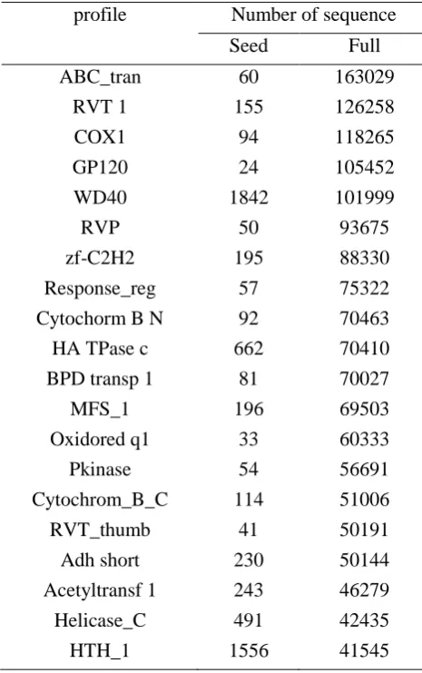
To evaluate the performance of generalized profile hidden Markov model, we use the top twenty protein families from the Pfam database (Table 1) which is a well-known database of protein families (15). Proteins are generally composed of one or more functional

(11)

125

Table 1. Top Twenty protein families in Pfam database profile Number of sequence

Seed Full

ABC_tran RVT 1 COX1 GP120 WD40 RVP zf-C2H2 Response_reg Cytochorm B N

HA TPase c BPD transp 1

MFS_1 Oxidored q1 Pkinase Cytochrom_B_C RVT_thumb Adh short Acetyltransf 1 Helicase_C HTH_1 60 155 94 24 1842 50 195 57 92 662 81 196 33 54 114 41 230 243 491 1556 163029 126258 118265 105452 101999 93675 88330 75322 70463 70410 70027 69503 60333 56691 51006 50191 50144 46279 42435 41545

There are two components in Pfam: Pfam-A and Pfam-B. The entries of the pfam-A have high quality and these twenty protein families belong to Pfam A. Pfam-A is the manually curated portion of the database. For each entry a protein sequence alignment and a hidden Markov model is stored. These hidden Markov models can be used to search sequence databases with the HMMER package written by Sean Eddy (2).

To assess the performance of the generalized PHMM, 20 sequences from each family are randomly removed. So we have 400 sequences removed in total. We consider these data as TEST sequences while the other sequences form the training set. Because of computational problem, we only repeat this procedure10 times.

Given the training sequences of twenty protein families, the transition matrix _{( ) ( )} and the emission matrix _{( )} are estimated using

generalized and common Baum-Welch algorithms. Then, each removed sequences (a sequence of TEST data) is returned to all families (not only that family which has been removed from). The log-likelihood value of each test sequence for all protein families is computed. Then the numbers of correctly assigned test sequences to the twenty protein families are counted (Table 2).

Table 2. The average numbers of correctly assigned sequences

Profiles Common

Baum-Welch

Generalized Baum-Welch

ABC_tran 10.6 18.7

RVT 1 14.3 18.8

COX1 12.5 16.0

GP120 18.3 18.3

WD40 14.0 16.2

RVP 12.0 18.7

zf-C2H2 6.3 18.9

Response_reg 14.8 16.3

Cytochorm B N 14.9 16.2

HA TPase c 14.0 18.4

BPD transp 1 14.0 16.4

MFS_1 16.5 16.1

Oxidored q1 16.3 16.9

Pkinase 6.1 14.4

Cytochrom_B_C 14.4 16.8

RVT_thumb 12.2 18.1

Adh short 10.6 14.6

Acetyltransf 1 12.7 18.1

Helicase_C 14.1 14.0

HTH_1 5.3 14.0

(12)

initial parameters carefully. We perform the algorithm with different initial parameters in a way that the transition probabilities into Match states are larger than transition probabilities into other states.

We also use the generalized Viterbi algorithm for determining the most probable path for each test sequence in corresponding protein family. Fort this purpose we use the following equation:

P( | ) ( ) ( ) or

( | ) ( ) ∑ ( ( ))

Equation 7 indicates the log-likelihood values of the optimal (most likely) sequence of hidden states for a test sequence. We calculate this score for all test sequences into each family using generalized and common Viterbi algorithm. We then normalized the log-likelihood values (scores) into each family. Figure 6 indicates that the average of normalized score for most probable path into each protein family obtained by considering the one-by-one dependency are higher than common Viterbi algorithm.

1. Rabiner, L.R., and Biing-Hwang, J. (1986) An introduction to hidden Markov models.

ASSP

Mag., IEEE

,

3 , 4-16.

2. Eddy, S.R. (1998) Profile hidden Markov models.

Bioinformatics

,

14 , 755-763.

3. Dymarski, P. (2011)

Hidden Markov Models, theory and applications

. InTech Open Access

Publishers.

4. Bilmes, J.A. (2003) Buried Markov models: A graphical-modeling approach to automatic speech

recognition.

Comput. Speech Lang.

,

17 , 213-231.

5. Bahl, L.R., Brown,

P.F., de Souza, P.V. and Mercer, R.L. (1986) Maximum mutual information

estimation of hidden Markov model parameters for speech recognition.

Proc. ICASSP

86, Pp. 49-52.

6. Selvaraj, L., and Ganesan, B. (2014) Enhancing speech recognition using improved particle

swarm optimization based Hidden Markov Model.

Scientific World J

. DOI:

10.1155/2014/270576

7. Shannon, M., Heiga Zen, H., and Byrne, W. (2013) Autoregressive models for statistical

parametric speech synthesis.

Audio, Speech, Lang. Proc., IEEE Trans.

,

21 , 587-597.

8. Sonnhammer, E.L.L, von Heijne, G. and Krogh, A. (1998) A hidden Markov model for

predicting transmembrane helices in protein sequences.

ISMB 98 Proceedings

,

Pp

. 1-8.

9. Holmes, I. (2003) Using guide trees to construct multiple-sequence evolutionary HMMs.

Bioinformatics

,

19 (suppl. 1), i147-i157.

10. Qian, B. and Goldstein, R.A. (2004) Performance of an iterated T-HMM for homology

detection.

Bioinformatics

,

20 , 2175-2180.

11. Siepel, A., and Haussler, D. (2004) Combining phylogenetic and hidden Markov models in

biosequence analysis.

J.Comput. Biol.

,

11 , 413-428.

12. Rabiner, L.R. (1989) A tutorial on Hidden Markov Models and selected applications in speech

recognition.

Proc. IEEE

,

77 , 257-285.

13. Viterbi, A.J. (1967) Error bounds for convolutional codes and an asymptotically optimum

decoding algorithm.

IEEE Transactions on

Information Theory

,

13 , 260-269.

(13)