A Max-Norm Constrained Minimization Approach to 1-Bit Matrix Completion

A Max-Norm Constrained Minimization Approach to 1-Bit Matrix

Completion

Tony Cai [email protected]

Statistics Department The Wharton School University of Pennsylvania Philadelphia, PA 19104, USA

Wen-Xin Zhou [email protected]

Department of Mathematics and Statistics University of Melbourne

Parkville, VIC 3010, Australia

Editor:Nathan Srebro

Abstract

We consider in this paper the problem of noisy 1-bit matrix completion under a general non-uniform sampling distribution using the max-norm as a convex relaxation for the rank. A max-norm con-strained maximum likelihood estimate is introduced and studied. The rate of convergence for the estimate is obtained. Information-theoretical methods are used to establish a minimax lower bound under the general sampling model. The minimax upper and lower bounds together yield the op-timal rate of convergence for the Frobenius norm loss. Computational algorithms and numerical performance are also discussed.

Keywords: 1-bit matrix completion, low-rank matrix, max-norm, trace-norm, constrained opti-mization, maximum likelihood estimate, optimal rate of convergence

1. Introduction

or negative rating. Similar problem also arises in analyzing incomplete survey designs containing simple agree/disagree questions in the analysis of survey data, and distance matrix recovery in multidimensional scaling that incorperates binary responses with incomplete data (Green and Wind, 1973; Spence and Demoney, 1974). See Davenport et al. (2012) for more discussions on potential applications.

Motivated by these applications, Davenport et al. (2012) considered the1-bit matrix completion problemof recovering an approximately low-rank matrix M∗_∈Rd1×d2 _{from a set of nnoise} cor-rupted sign (1-bit) measurements. In particular, they proposed a trace-norm constrained maximum likelihood estimator to estimateM∗, based on a small number of binary samples observed according to a probability distribution determined by the entries ofM∗. It was also shown that the trace-norm constrained optimization method is minimax rate-optimal under the uniform sampling model. This problem is closely connected to and in some respects more challenging than the1-bit compressed sensing, which was introduced and first studied in Boufounos and Baraniuk (2008). The 1-bit mea-surements are meant to model quantization in the extreme case, and a surprising fact is that when the signal-to-noise ratio is low, empirical evidence demonstrates that such extreme quantization can be optimal when constrained to a fixed bit budget (Laska and Baraniuk, 2012). See Plan and Vershynin (2013a) for the recent results and references on 1-bit compressed sensing.

To be more specific, consider an arbitrary unknownd1_×d2target matrixM∗with rank at most r. Suppose a subsetS=_{(i1,j1), ...,(in,jn)}of entries of a binary matrixY is observed, where the entries ofY depend onM∗in the following way:

Yi,j=

+1, ifM_i∗_,j+Zi,j≥0,

−1, ifM_i∗_,j+Zi,j<0.

Here Z = (Zi j)∈Rd1×d2 is a general noise matrix. This latent variable matrix model can been seen as a direct analogue to the usual 1-bit compressed sensing model, in which only the signs of measurements are observed. It is known that ans-sparse signal can still be approximately recovered fromO(slog(d/s))random linear measurements. See, for example, Jacques et al. (2011), Plan and Vershynin (2013a), Plan and Vershynin (2013b) and Ai et al. (2013).

Contrary to the standard matrix completion model and many other statistical problems, random noise turns out to be helpful and has a positive effect in the 1-bit case, since the problem is ill-posed in the absence of noise as described in Davenport et al. (2012). In particular, when Z=0 and M∗=uvT for some vectors u_∈Rd1_,v∈Rd2 _{having no zero coordinates, then the radically} disparate matrixMe=sign(u)signT_{(v) will lead to the same observationsY. Thus M andMe are} indistinguishable. However, it has been surprisingly noticed that the problem may become well-posed when there are some additional stochastic variations, that is,Z₆=0 is an appropriate random noise matrix. This phenomenon can be regarded as a “dithering” effect brought by random noise.

so-calledmax-norm(Linial et al., 2007), which is defined by

kM_kmax= min M=UVT

kU_k2,∞kVk2,∞ , (1)

where the infimum is over all factorizations M=UVT with _kU_k2,∞ being the operator norm of U :ℓk

2→ℓd∞1 and kVk2,∞ the operator norm ofV :ℓ₂k →ℓd∞2 (or, equivalently,VT :ℓd12 →ℓk2) and k=1, ...,min(d1,d2). It is not hard to check thatkUk2,∞is equal to the largestℓ2norm of the rows inU. Sinceℓ2is a Hilbert space,k·kmaxindeed defines a norm on the space of operators betweenℓd12 andℓd1

∞. Comparably, the trace-norm has a formulation similar to(1), as given below in Section 2.1. Foygel and Srebro (2011) first used the max-norm for matrix completion under the uniform sampling distribution. Their results are direct consequences of a recent bound on the excess risk for a smooth loss function, such as the quadratic loss, with a bounded second derivative (Srebro et al., 2010). Matrix completion under a non-degenerate random sampling model was studied in Cai and Zhou (2013), where it was shown that the max-norm constrained minimization method is rate-optimal and it yields a more stable approximate recovery guarantee, with respect to the sampling distributions, than trace-norm based approaches.

Davenport et al. (2012) analyzed 1-bit matrix completion under theuniform sampling model, where observed entries are assumed to be sampled randomly and uniformly. In such a setting, the trace-norm constrained approach has been shown to achieve minimax rate of convergence. However, in certain application such as collaborative filtering, the uniform sampling model is over idealized. In the Netflix problem, for instance, the uniform sampling model is equivalent to assuming all users are equally likely to rate every movie and all movies are equally likely to be rated by any user. In practice, inevitably some users are more active than others and some movies are more popular and thus rated more frequently. Therefore, the sampling distribution is in fact non-uniform. In this scenario, Salakhutdinov and Srebro (2010) showed that the standard trace-norm relaxation can behave very poorly, and suggested to use a weighted variant of the trace-norm, which takes the sampling distribution into account. Since the true sampling distribution is most likely unknown and can only be estimated based on the locations of those entries that are revealed in the sample, what commonly used in practice is the empirically-weighted trace norm. Foygel et al. (2011) pro-vided rigorous recovery guarantees for learning with the standard weighted, smoothed weighted and smoothed empirically-weighted trace-norms. In particular, they gave upper bounds on excess error, which show that there is no theoretical disadvantage of learning with smoothed empirical marginals as compared to learning with smoothed true marginals.

re-spect to the sampling distributions, while previously used approaches are based on different variants of the trace-norm which may sometimes seem artificial to practitioners.

When the noise distribution is Gaussian or more generally log-concave, the negative log-likelihood function forM, given the measurements, is convex, hence computing the max-norm constrained maximum likelihood estimate is a convex optimization problem. The computational effectiveness of this method is also studied, based on a first-order algorithm developed in Lee et al. (2010) for solving convex programs involving a max-norm constraint, which outperforms the semi-definite programming method used in Srebro et al. (2005). It will be shown in Section 4 that the convex optimization problem can be implemented in polynomial time as a function of the sample size and the matrix dimensions.

The rest of the paper is organized as follows. Section 2 begins with the basic notation and def-initions, and then states a collection of useful results on the matrix norms, Rademacher complexity and distances between matrices that will be needed throughout the paper. Section 3 introduces the 1-bit matrix completion model and the estimation procedure and investigates the theoretical proper-ties of the estimator. Both minimax upper and lower bounds are established. The results show that the max-norm constraint maximum likelihood estimator is rate-optimal over the parameter space. Section 3 also gives a comparison of our results with previous work. Computational algorithms are discussed in Section 4, and numerical performance of the proposed algorithm is presented in Section 5. The paper is concluded with a brief discussion in Section 6, and the proofs of the main results are given in Section 7.

2. Notations and Preliminaries

In this section, we introduce basic notation and definitions that will be used throughout the paper, and state some known results on the max-norm, trace-norm and Rademacher complexity that will be used repeatedly later.

2.1 Notation

For any positive integerd, we use[d]to denote the set of integers_{1,2, ...,d_}. For any pair of real numbersaandb, seta_∨b:=max(a,b)anda_∧b:=min(a,b). For a vectoru_∈Rdand 0<p<∞, denote itsℓp-norm bykukp= (∑di=1|ui|p)1/p. In particular,kuk∞=maxi=1,...,d|ui|is theℓ∞-norm. For a matrix M= (Mk,l)∈Rd1×d2, letkMkF =

q

∑d1

k=1∑ d2

l=1M2k,l be the Frobenius norm and let

kM_k∞=maxk,l|Mk,l|denote the elementwise ℓ∞-norm. Given two normsℓp andℓq on Rd1 and

Rd2 _{respectively, the corresponding operator normk · k}

p,q of a matrix M∈Rd1×d2 is defined by

kM_kp,q=sup_kxkp=1kMxkq. It is easy to verify thatkMkp,q=kMTkq∗_,p∗, where(p,p∗)and(q,q∗)

are conjugate pairs, that is, 1_p+_p1∗ =1 and 1_q+_q1∗ =1. In particular,kMk=kMk2,2is the spectral norm and_kMk2,∞=maxk=1,...,d1

q

∑d2

2.2 Max-Norm and Trace-Norm

For any matrixM∈Rd1×d2_{, itstrace-normis defined to be the sum of the singular values ofM(that} is, the roots of the eigenvalues ofMMT), and can also equivalently written as

kM_k∗=inf

∑

j

|σj|:M=

∑

j

σjujvTj,uj∈Rd1,vj∈Rd2 satisfyingkujk2=kvjk2=1

.

Recall the definition(1) of the max-norm, the trace-norm can be analogously defined in terms of matrix factorization as

kMk∗= min M=UVT

kUkFkVkF = 1

2U,V:minM=UVT kUk 2

F+kVk2F

.

Since theℓ1-norm of a vector is bounded by the product of itsℓ2-norm and the number of non-zero coordinates, we have the following relationship between the trace-norm and Frobenius norm

kM_kF ≤ kMk∗≤

p

rank(M)_{· k}M_kF.

By the elementary inequality_kMm×nkF≤√mkMm×nk2,∞, we see that

kM_k∗

√

d1d2 ≤ k

M_kmax. (2)

Furthermore, as was noticed in Lee et al. (2010), the max-norm, which is defined in(1), is compa-rable with a trace-norm more precisely in the following sense (Jameson, 1987):

kM_kmax (3)

≈inf

∑

j

|σj|:M=

∑

j

σjujvTj,uj∈Rd1,vj∈Rd2 satisfyingkujk∞=kvjk∞=1

,

where the factor of equivalence isKG∈(1.67,1.79), denoting the Grothendieck’s constant. What may be more surprising is the following bounds for the max-norm, in connection with element-wise

ℓ∞-norm (Linial et al., 2007):

kM_k∞≤ kMkmax≤

p

rank(M)_{· k}M_k1,∞≤

p

rank(M)_{· k}M_k∞. (4)

2.3 Rademacher Complexity

Considering matrices as functions from index pairs to entry values, a technical tool used in our proof involves data-dependent estimates of theRademacher complexityof the classes that consist of low trace-norm and low max-norm matrices. We refer to Bartlett and Mendelson (2002) for a detailed introduction of this concept.

Definition 1 Let

P

be a probability distribution on a set

X

. Suppose that X1, ...,Xnare independent samples drawn from

X

according to

P

, and set S=_{X1, ...,Xn}. For a class

F

of functions mapping from

X

toR, its empirical Rademacher complexity over the sample S is defined by

b

RS(

F

) = 2

|S_|Eε

h

sup f∈F

n

∑

i=1

εif(Xi)

whereε= (ε1, ...,εn)is a Rademacher sequence. The Rademacher complexity with respect to the distribution

P

is the expectation, over a sample S of_|S_|points drawn i.i.d. according to

P

, denoted by

R_|S_|(

F

) =ES∼P[RbS(

F

)].

The following properties regardingRbS(

F

)are useful.

Proposition 2 We have

1. If

F

⊆

G

,RbS(

F

)≤RbS(

G

).

2. RbS(

F

) =RbS(conv(

F

)) =RbS(absconv(

F

)), whereconv(

F

)is the class of convex combina-tions of funccombina-tions from

F

, andabsconv(

F

)denotes the absolutely convex hull of

F

, that is, the class of convex combinations of functions from

F

and₋

F

.

3. For every c_∈R,RbS(c

F

) =|c|RbS(

F

), where c

F

≡ {c f : f∈

F

}.

In particular, we are interested in calculating the Rademacher complexities of the trace-norm and max-norm balls. To this end, define for any radiusR>0 that

B∗(R) := M∈Rd1×d2:kMk∗≤R and

Bmax(R) :=

M∈Rd1×d2_:kMk

max≤R .

First, recall that any matrix with unit trace-norm is a convex combination of unit-norm rank-one matrices, and thus

B∗(1) =conv(

M

1), where

M

1:=uvT :u∈Rd1,v∈Rd2,kuk2=kvk2=1 . (5) Then RbS(B∗(1)) =RbS(

M

1). A sharp bound on the worst-case Rademacher complexity, defined as the supremum ofRbS(·) over all sample setsS with size |S|=n, is √2_n (See, expression (4) on page 551, Srebro and Shraibman, 2005). This bound, unfortunately, is barely useful in developing generalization error bounds. However, when the index pairs of a sampleSare drawn uniformly at random from[d1]×[d2](with replacement), Srebro and Shraibman (2005) showed that theexpected Rademacher complexity is low, and Foygel and Srebro (2011) have improved this result by reducing the logarithmic factor. In particular, they proved that for a sample sizen_≥d=d1+d2,

ES_∼unif,|S_|=n

_b

RS(B∗(1))≤ K

√

d1d2

r

dlog(d) n ,

whereK>0 denotes a universal constant.

The unit max-norm ball, on the other hand, can be approximately characterized as a convex hull. Due to the Grothendieck’s inequality, it was shown in Srebro and Shraibman (2005) that

conv(

M

_±)_⊂Bmax(1)⊂KG·conv(

M

±),

|

M

_±|=2d−1_{,d=d1+d2. For anyd1,d2>2 and any sample of size 2<|S| ≤d1d2, the empirical} Rademacher complexity of the unit max-norm ball is bounded by

b

RS Bmax(1)

≤12

s

d

|S_|. (6)

In other words, sup_S:|S|=nRbS(Bmax(1))≤12

q

d n.

2.4 Discrepancy

In order to get both upper and lower prediction error bounds on the weighted squared Frobenius norm between the proposed estimator, given by (13) below, and the target matrix described via model(9), we will need the following two concepts of discrepancies between matrices as well as their connections. In particular, we will focus on element-wise notion of discrepancy between two d1_×d2matricesPandQ.

First, for two matricesP,Q:[d1]_×[d2]_→[0,1]d1×d2_{, their Hellinger distance is given by}

d_H2(P;Q) = 1 d1d2₍

∑

_k,l)

d_H2(Pk,l;Qk,l),

whered_H2(p;q) = (√p₋√q)2_{+ (}√_1−p−√_1−q)2 _{for p,q∈[0,1]. Next, the Kullback-Leibler} divergence between two matricesP,Q:[d1]×[d2]→[0,1]d1×d2 is defined by

K(P_kQ) = 1

d1d2₍

∑

_k,l)K(Pk,lkQk,l),

whereK(p_kq) =plog(p_q) + (1₋p)log(1₁−_−qp), forp,q_∈[0,1]. Note thatK(P_kQ)is not a distance; it is sufficient to observe that it is not symmetric.

The relationship between the two “distances” is as follows. For any two scalarsp,q_∈[0,1], we have

d_H2(p;q)_≤K(p_kq), (7)

which in turn implies that, for any two matricesP,Q:[d1]_×[d2]_→[0,1]d1×d2_,

d2_H(P;Q)_≤K(P_kQ). (8)

The proof of(7)is based on the Jensen’s inequality and an elementary inequality that 1₋x_{≤ −}logx for anyx>0.

3. Max-Norm Constrained Maximum Likelihood Estimate

3.1 Observation Model

We consider 1-bit matrix completion under a general random sampling model. The unknown low-rank matrix M∗_∈Rd1×d2 _{is the object of interest. Instead of observing noisy entries M}∗

i,j+Zi,j directly inunquantized matrix completion, now we only observe with error the sign of a random subset of the entries ofM∗. More specifically, assume that a random sample

S=(i1,j1),(i2,j2), ...,(in,jn) ⊆ [d1]×[d2]

n

of the index set is drawn i.i.d. with replacement according to a general sampling distributionΠ=

{πkl}on[d1]×[d2]. That is,P{(it,jt) = (k,l)}=πkl, for allt and(k,l). Suppose that a (random) subset S of size _|S_|=n of entries of a sign matrixY is observed. The dependence of Y on the underlying matrixM∗is as follows:

Yi,j=

+1, ifM_i∗_,j+Zi,j≥0,

−1, ifM_i∗_,j+Zi,j<0,

(9)

whereZ= (Zi,j)∈Rd1×d2 is a matrix consisting of i.i.d. noise variables. LetF(·)be the cumulative distribution function of₋Z1,1, then the above model can be recast as

Yi,j=

+1, with probabilityF(M_i∗_,j),

−1, with probability 1₋F(M∗_i,j), (10)

and we observe noisy entries _{Yit,jt} n

t=1 indexed by S. More generally, we consider the model (10)with an arbitrary differentiable function F:R→[0,1]. Particular assumptions onF will be discussed below.

Instead of assuming the uniform sampling distribution as in Davenport et al. (2012), here we al-low a general sampling distributionΠ=_{πkl}, satisfying∑(k,l)∈[d1]×[d2]πkl=1, according to which we makenindependent random choices of entries. The drawback of the setting is that, with fairly high probability, some entries will be sampled multiple times. Intuitively it would be more practical to assume that entries are sampled without replacement, or equivalently, to samplenof thed1d2 bi-nary entries observed with noise without replacing. Due to the requirement that the drawn entries be distinct, thensamples are not independent. This dependence structure turns out to impede the tech-nical analysis of the learning guarantees. To avoid this complication, we will use the i.i.d. approach as a proxy for sampling without replacement throughout this paper. As has been noted in Gross and Nesme (2010) and Foygel and Srebro (2011), between sampling with and without replacement both in a uniform sense, that is, makingnindependent uniform choices of entries versus choosing a set Sof entries uniformly at random over all subsets that consist of exactlynentries, the latter can be theoretically as good as the former. See Section 7.4 below for more details.

Next we list three natural choices forF, or equivalently, for the distribution of_{Zi,j}.

3.1.1 EXAMPLES

1. (Logistic regression/Logistic noise): The logistic regression model is described by(10)with

F(x) = e x

1+ex,

2. (Probit regression/Gaussian noise): The probit regression model is described by(10)with

F(x) =Φx σ

,

whereΦdenotes the cumulative distribution function ofN(0,1), and equivalently by(9)with Zi,j i.i.d. followingN(0,σ2).

3. (Laplacian noise): Another interesting case is that the noise Zi,j are i.i.d. drawn from a Laplacian distribution Laplace(0,b), with

F(x) =

1

2exp(x/b), ifx<0, 1₋1₂exp(₋x/b), ifx_≥0,

whereb>0 is the scale parameter.

Davenport et al. (2012) have focused on approximately low-rank matrices recovery by consid-ering the following class of matrices

K_∗(α,r) =nM_∈Rd1×d2 _:kMk

∞≤α, k M_k∗

√

d1d2 ≤

α√ro, (11)

where 1_≤r_≤min(d1,d2)andα>0 is a free parameter to be determined. Clearly, any matrixM with rank at mostr satisfying _kM_k∞≤α belongs to K∗(α,r). Alternatively, using max-norm as a convex relaxation for the rank, we consider recovery of matrices with ℓ∞-norm and max-norm constraints defined by

Kmax(α,R):=nM_∈Rd1×d2 _:kMk

∞≤α,kMkmax≤R

o

. (12)

Here bothα>0 andR>0 are free parameters to be determined. IfM∗ is of rank at mostr and

kM∗_k∞≤α, then by(2)and(4)we haveM∗∈Bmax(α√r)and hence M∗_∈Kmax(α,α√r)_⊂K_∗(α,r).

3.2 Max-norm Constrained Maximum Likelihood Estimate Now, given a collection of observationsYS={Yit,jt}

n

t=1from the observation model(10), the nega-tive log-likelihood function can be written as

ℓS(M;Y) = n

∑

t=1

1_{Y

it,jt=1}log

₁

F(Mit,jt)

+1_{Y

it,jt=−1}log

₁

1₋F(Mit,jt)

.

Then we consider estimating the unknownM∗_∈Kmax(α,R)by maximizing the empirical likelihood function subject to a max-norm constraint:

b

Mmax= arg min

M∈Kmax(α,R)

ℓS(M;Y). (13)

matrix recovery problems by controlling thespikinessof the solution. Indeed, the measure of the “spikiness” of matrices is much less restrictive than the incoherence conditions imposed in exact low-rank matrix recovery. See, for example, Koltchinskii et al. (2011), Negahban and Wainwright (2012), Klopp (2012) and Cai and Zhou (2013).

As has been noted in Srebro et al. (2005), a large gap between the max-complexity (related to max-norm) and the dimensional-complexity (related to rank) is possible only when the underlying low-rank matrix has entries of vastly varying magnitudes. Also, in view of (3), the max-norm promotes low-rank decomposition with factors in ℓ∞ (ℓ2 for the trace-norm). Motivated by these features, max-norm regularization is expected to be reasonably effective for uniformly bounded data.

When the noise distribution is log-concave so that the log-likelihood is a concave function, the max-norm constrained minimization problem(13)is a convex program and we recommend a fast and efficient algorithm developed in Lee et al. (2010) for solving large-scale optimization problems that incorporate the max-norm. We will show in Section 4 that the convex optimization problem (13)can indeed be implemented in polynomial time as a function of the sample sizenand the matrix dimensionsd1andd2.

3.3 Upper Bounds

To establish an upper bound on the prediction error of estimatorMmaxb given by(13), we need the following assumption on the unknown matrixM∗as well as the regularity conditions on the function Fin(10).

3.3.1 CONDITIONU

Assume that there exist positive constantsRandαsuch that

(U1) M∗_∈Kmax(α,R);

(U2) FandF′ are non-zero in[₋α,α], and

(U3) both

Lα:= sup |x|≤α

|F′(x)_|

F(x)(1₋F(x)), and βα:=_|sup_x|≤α

F(x)(1₋F(x))

(F′_(x))2 (14) are finite.

In particular, under condition (U2), the quantity

Uα:= sup |x|≤α

log

1 F(x)(1₋F(x))

,

is well-defined. As prototypical examples, we specify below the quantities Lα, βα andUα in the cases of Logistic, Gaussian and Laplacian noise:

1. (Logistic regression/Logistic noise): ForF(x) =ex/(1+ex), we have

Lα≡1, βα= (1+e α₎2

eα and Uα=2 log(e

2. (Probit regression/Gaussian noise): For F(x) =Φ(x/σ), straightforward calculations show that

Lα≤ 4

σ

_α

σ+1

, βα≤πσ2exp{α2/(2σ2)} and Uα≤

_α

σ+1

2

. (15)

3. (Laplacian noise): For a Laplace(0,b)distribution function, we have

Lα= 2

b, βα=b 2 exp(α/b)−1

and Uα≤2

_α

b+log 2

.

Now we are ready to state our main results concerning the recovery of an approximately low-rank matrixM∗using the max-norm constrained maximum likelihood estimate. We write hereafter d=d1+d2for brevity.

Theorem 3 Suppose that Condition U holds and assume that the training set S follows a general weighted sampling model according to the distributionΠ. Then there exists an absolute constant C such that, for a sample size2<n_≤d1d2and for anyδ>0, the minimizerMmaxb of the optimization program(13)satisfies

kMmaxb −M∗k2 Π=

d1

∑

k=1

d2

∑

l=1

πkl{Mbmax−M∗}2k,l≤Cβα

LαR

r

d n+Uα

r

log(4/δ) n

, (16)

with probability at least 1₋δ. Here and below_{k · k}Π denotes the weighted Frobenius norm with respect toΠ, that is,

kM_kΠ=

v u u t

_∑

d1

k=1 d2

∑

l=1

πklM_k2_,l for all M∈Rd1×d2.

Remark 4 (i) While using the trace-norm to study this general weighted sampling model, it is common to assume that each row and column is sampled with positive probability (Klopp, 2012; Negahban and Wainwright, 2012), though in some applications this assumption does not seem realistic. More precisely, assume that there exists a positive constantµ_≥1 such that

πkl≥

1 µd1d2

, for all(k,l)_∈[d1]×[d2]. (17)

Then, under condition(17)and the conditions of Theorem 3,

1 d1d2k

b

Mmax₋M∗_k2_F≤Cµβα

LαR

r

d n+Uα

r

log(d) n

(18)

holds with probability at least 1₋4/d, whereC>0 denotes an absolute constant.

It is noteworthy that above results are directly comparable to those obtained in the case of ap-proximately low-rank recovery from unquantized measurements, also using max-norm regularized approach (Cai and Zhou, 2013). LetZ= (Zi,j)be a noise matrix consisting of i.i.d.N(0,σ2)entries for someσ>0, and assume we have observations on a (random) subsetS=_{(i1,j1), ...,(in,jn)}of entries ofYe=M∗+Z. Cai and Zhou (2013) studied the unquantized problem under a general sam-pling model using max-norm as a convex relaxation for the rank. In particular, for the max-norm constrained least squares estimator

e

Mmax= arg min

M∈Kmax(α,R) 1 n

n

∑

t=1

(Yeit,jt−Mi∗t,jt) 2_,

forKmax(α,R)as in(12), it was shown that for anyδ_∈(0,1)and a sample size 2<n_≤d1d2,

kMemax−M∗k2Π≤C′

(α_∨σ)R

r

d n+

α2_log(2/δ) n

(19)

holds with probability greater than 1₋exp(₋d)₋δ, whereC′>0 is a universal constant.

In 1-bit observations case whenZi,j i.i.d.

∼ N(0,σ2_{), it is equivalent that the functionF in model} (10)is given byF(_·) =Φ(_·/σ). According to(15), we have

kMmaxb ₋M∗_k2_Π≤Cexp

_α2

2σ2

(α+σ)R

r

d

n+ (α+σ) 2

r

log(4/δ) n

(20)

holds with probability at least 1₋δ.

Comparing the upper bounds in(19)and(20)and note thatα_∨σ_≤α+σ_≤2(α_∨σ), we see that there is no essential loss of recovery accuracy by discretizing to binary measurements as long as α_σ is bounded by a constant (Davenport et al., 2012). On the other hand, as the signal-to-noise ratio α_{σ ≥}1 increases, the error bounds deteriorate significantly. In fact, the caseα_≫σessentially amounts to the noiseless setting, in which it is impossible to recoverM∗based on any subset of the signs of its entries.

3.4 Information-Theoretic Lower Bounds

We now establish minimax lower bounds by using information-theoretic techniques. The lower bounds given in Theorem 5 below show that the rate attained by the max-norm constrained maxi-mum likelihood estimator is optimal up to constant factors.

Theorem 5 Assume that F′(x)is decreasing and F(x₍)(_F′1₍−_x))F2(x)) is increasing for x>0, and let S be any subset of[d1]×[d2]with cardinality n. Then, as long as the parameters(R,α)satisfy

max

2, 4

(d1∨d2)1/2

≤R

α ≤

(d1∧d2)1/2

2 ,

the minimax risk for estimating M over the parameter space Kmax(α,R)satisfies

inf b

M

max M∈Kmax(α,R)

₁

d1d2EkMb−Mk 2 F

≥₅₁₂1 min

α2_,

q

β_α/2

2 R

r

d n

Remark 6 In fact, the lower bound(21)is a special case of the following general result, which will be proved in Sect. 7.2. Letγ∗>0 be the solution of the following equation

γ∗=min

1 2,

R1/2

α

_β

(1−γ∗_)α

32 ·

d1∨d2 n

1/4

(22)

and assume that

max

2, 4

(d1_∨d2)1/2

≤R_α ≤(d1_∧d2)1/2γ∗. (23) Then the minimax risk for estimatingMover the parameter spaceKmax(α,R)satisfies

inf b

M

max M∈Kmax(α,R)

1 d1d2Ek

b

M₋M_k2_F

≥₅₁₂1 min

α2,

q

β(1−γ∗_)α

2 R r d n . (24)

To see the existence ofγ∗defined above, setting

h(γ) =γ and g(γ) =min

1 2,

R1/2

α

_β

(1₋γ)α

32 ·

d1_∨d2 n

1/4

,

then it is easy to see thath(γ)is strictly increasing andg(γ)is decreasing forγ_∈(0,1)withh(0) =0 andg(0)>0. Therefore, equation(22)has a unique solutionγ∗_∈(0,1₂]so thath(γ∗) =g(γ∗).

Assume thatµandαare bounded above by universal constants and let the functionF be fixed, so that both Lα and βα in (14) are bounded. Also notice that β(1−γ∗_)α≥β_α/2 since γ∗ ≤1/2.

Then comparing the lower bound (24) with the upper bound (18) shows that if the sample size

n_≥R 2_β

α/2

4α4 (d1+d2), the optimal rate of convergence isR

q

d1+d2

n :

inf b

M

sup M∈Kmax(α,R)

1

d1d2EkMb−Mk 2 F≍R

r

d1+d2 n ,

and the max-norm constrained maximum likelihood estimate (13) is rate-optimal. If the target matrixM∗is known to have rank at mostr, we can takeR=α√r, such that the requirement here on

the sample sizen_≥βα/2

4α2r(d1+d2)is weak and the optimal rate of convergence becomesα

q

r(d1+d2)

n .

3.5 Comparison to Prior Work

In this paper, we study a matrix completion model proposed in Davenport et al. (2012), in which it is assumed that a binary matrix is observed at random from a distribution parameterized by an unknown matrix which is (approximately) low-rank. It is noteworthy that some earlier papers on collaborative filtering or matrix completion, including Srebro et al. (2005) and references therein, also dealt with binary observations that are assumed to be noisy versions of the underlying matrix, in Logistic or Bernoulli conditional model. The goal there is to predict directly the quantized values, or equivalently, to reconstruct the sign matrix, instead of the underlying real values, therefore the non-identifiability issue could be avoided.

a proxy to rank, Davenport et al. (2012) have studied 1-bit matrix completion under theuniform sampling distributionover the parameter spaceK_∗(α,r)as given in(11), for someα>0 andr_≤ min_{d1,d2} is a positive integer. To recover the unknown M∗∈K∗(α,r), given a collection of observationsYSwhereSfollows a Bernoulli model, that is, every entry(k,l)∈[d1]×[d2]is observed independently with equal probability _dn

1d2, they propose the following trace-norm constrained MLE

b

Mtr= arg min M∈K∗(α,r)

ℓS(M;Y)

and prove that for a sample sizen_≥dlog(d),d=d1+d2, with high probability,

1 d1d2k

b

Mtr₋M∗_k2_F .βαLαα

r

rd

n. (25)

Comparing to (18) with R=α√r, it is easy to see that under the uniform sampling model, the error bounds in (rescaled) Frobenius norm for the two estimates Mmaxb and Mtrb are of the same order. Moreover, Theorem 3 in Davenport et al. (2012) and Theorem 5, respectively, provide lower bounds showing that both Mtrb andMmaxb achieve the minimax rate of convergence for recovering approximately low-rank matrices over the parameter spacesK_∗(α,r)andKmax(α,R)respectively.

As mentioned in the introduction, the uniform sampling distribution assumption is restrictive and not valid in many applications including the well-known Netflix problem. When the sampling distribution is non-uniform, it was shown in Salakhutdinov and Srebro (2010) that the standard trace-norm regularized method might fail, specifically in the setting where the row and column marginal distributions are such that certain rows or columns are sampled with very high probabil-ities. Moreover, it was proposed to use a weighted variant of the trace-norm, which incorporates the knowledge of the true sampling distribution in its construction, and showed experimentally that this variant indeed leads to superior performance. Using this weighted trace-norm, Negahban and Wainwright (2012) provided theoretical guarantees on approximate low-rank matrix completion in general sampling case while assuming that each row and column is sampled with positive probabil-ity (see condition(17)). In addition, requiring that the probabilities to observe an element from any row or column are of orderO((d1∧d2)−1), Klopp (2012) analyzed the performance of the trace-norm penalized estimators, and provided near-optimal (up to a logarithmic factor) bounds which are similar to the bounds in this paper.

Next we provide an analysis of the performance of the weighted trace-norm in 1-bit matrix completion. Given the knowledge of the true sampling distribution, we establish an upper bound on the error in recoveringM∗, which comparing to(25), includes an additional log1/2_{(d)factor. We do} not rule out the possibility that this logarithmic factor might be an artifact of the technical tools used in proof described below. The proof in Davenport et al. (2012) for the trace-norm regularization in uniform sampling case may also be extended to the weighted trace-norm method under the general sampling model, by using the matrix Bernstein inequality instead of Seginer’s theorem. The extra logarithmic factor, however, is still inevitable based on this argument. We will not pursue the details in this paper.

Given a sampling distributionΠ=_{πkl}on[d1]×[d2], define its row- and column-marginals as

πk·=

d2

∑

l=1

πkl and π·l=

d1

∑

k=1

respectively. Under the condition(17), we have

πk·≥

1 µd1

, π_·l ≥ 1 µd2

, for all(k,l)_∈[d1]_×[d2]. (26)

As in Salakhutdinov and Srebro (2010), consider the following weighted trace-norm with respect to the distributionΠ:

kM_kw,∗:=kMwk∗=diag(√π1·, ...,√πd1·)·M·diag(

√

π_·1, ...,√π·d2)

∗, (27)

where(Mw)k,l:=√πk_·π_·lMk,l. Notice that ifMhas rank at mostrandkMk∞≤α, then

kM_kw,∗≤√rkMkF=

√

r

d1

∑

k=1

d2

∑

l=1

πk·π·lM2k,l

1/2

≤α√r.

Analogously to the previous studied classK_∗(α,r), as given in(11), containing the low trace-norm matrices, define

KΠ,∗≡KΠ,∗(r,α) =

n

M_∈Rd1×d2_:kMk

w,∗≤α√r,kMk∞≤α

o

and consider estimating the unknownM∗_∈KΠ,∗by solving the following optimization problem:

b

Mw,tr=arg min M∈KΠ,∗

ℓS(M;Y). (28)

The following theorem states that the weighted trace-norm regularized approach can be nearly as good as the max-norm regularized estimator (up to logarithmic and constant factors), under a general sampling distribution that is not too far from uniform. The theoretical performance of the weighted trace-norm is first studied by Foygel et al. (2011) in the standard matrix completion problems under arbitrary sampling distributions.

Theorem 7 Suppose that Condition U holds but with M∗_∈KΠ,∗, and assume that the training set S follows a general weighted sampling model according to the distributionΠsatisfying(17). Then there exists an absolute constant C>0such that, for a sample size n_≥µmin_{d1,d2}log(d)and anyδ>0, the minimizerMbw,trof the optimization program(28)satisfies

kMbw,tr−M∗k2Π≤Cβα

Lαα

r

µrdlog(d) n +Uα

r

log(4/δ) n

, (29)

with probability at least1₋δ.

Since the construction of weighted trace-norm_{k · k}w,∗ highly depends on the underlying sam-pling distribution which is typically unknown in practice, the constraint M∗ ∈KΠ,∗ seems to be artificial. The max-norm constrained approach, on the contrary, does not require the knowledge of the exact sampling distribution and the error bound in weighted Frobenius norm, as shown in(16), holds even without prior assumption onΠ, for example, condition(17). Moreover, to ensure that the weighted trace-norm regularized method performs well, it is necessary that the marginals are not too small or equivalently that

µ=max

1 d1πk·∨

1 d2π_·l

:k,l_∈[d1]_×[d2]

is not too large. Otherwise, both the error bounds in (29) and the sample complexity µmin_{d1,d2_}log(d) would grow larger with µ when the marginals were far from uniform. We conjecture that the factorµwould also appear in the results that are extended from those in Daven-port et al. (2012). As evident in Theorem 3, using the max-norm based regularization does not lead to a deterioration in either the error bounds or the sample complexity when the sampling distribution was far from uniform.

To clarify the major difference between the principles behind (25) and (29), we remark that one of the key technical tools used in Davenport et al. (2012) is a bound of Seginer (2000) on the spectral norm of a random matrix with i.i.d. zero mean entries (corresponding to the uniform sampling distribution), that is, for anyh_≤2 log(max_{d1,d2}),

E[_kAkh_]≤Kh

E

h

max k=1,...,d1

kak·kh2

i

+_Eh max j=1,...,d2

ka_·lkh2

i

,

whereak· (resp. a·l) denote the rows (resp. columns) ofAandK is a universal constant. Under the non-uniform sampling model, we will deal with a matrix with independent entries that are not necessarily identically distributed, to which case an alternative result of Latala (2005) can be applied, that is,

E[_kA_k]_≤K′ max

k=1,...,d1Ek

ak_·k2+ max j=1,...,d2Ek

a_·lk2+

∑

k,l

Ea4_kl1/4i,

or instead, resorting to the matrix Bernstein inequality. Using either inequality would thus bring an additional logarithmic factor, appeared in(29).

It is also worth noticing that though the sampling distribution is not known exactly in practice, its empirical analogues are expected to be stable enough as an alternative. According to Foygel et al. (2011), given a random sampleS=_{(it,jt)}nt=1, consider the empirical marginals

b

πr(i) =#{t:it=i} n , bπ

c_{(j) =}#{t: jt= j}

n and bπi j=bπ

r_(i)bπc_(j),

as well as the smoothed empirical marginals

ˇ

πr_{(i) =}1 2(bπ

r_{(i) +1/d}

1), bπc(j) = 1 2(bπ

c_{(j) +1/d}

2) and ˇπi j=πˇr(i)πˇc(j).

The smoothed empirically-weighted trace-norm_{k · k}wˇ,∗ can be defined in the same spirit as in the definition (27) of weighted trace-norm, only with _{πi j} replaced by {πˇi j}. Then the unknown matrix can be estimated via regularization on the ˇπ-weighted trace-norm, that is,

ˇ

Mwˇ,tr=arg min

ℓS(M;Y):kMk∞≤α,kMkwˇ,∗≤α√r .

Adopting Theorem 4 in Foygel et al. (2011) to the current 1-bit problem will lead to a learning guarantee similar to(29).

4. Computational Algorithm

method (Lee et al., 2010). The first two are convex methods with guaranteed convergence rates to the global optimum, though can be slow in practice and might not scale to matrices with hundreds of rows or columns. We describe in this section a simple first order method due to Lee et al. (2010), which is a special case of a projected gradient algorithm for solving large-scale convex programs involving the max-norm. This method is non-convex, but as long as the size of the problem is large enough, it is guaranteed that each local minimum is also a global optimum, due to Burer and Monteiro (2003).

We start from rewriting the original problem as an optimization over factorizations of a matrix M_∈Rd1×d2_{into two termsM=UV}T_{, whereU∈R}d1×k_andV∈Rd2×k_{for some 1≤k≤d=d}

1+d2. More specifically, for any 1_≤k≤dfixed, define

M

k(R):=

n

UVT:U_∈Rd1×k_{,V ∈R}d2×k_,max{kUk2

2,∞,kVk22,∞} ≤R

o

.

Then the global optimum of(13)is equal to that of

minimize ℓ(M;Y)

subject to M_∈

M

k(R), kMk∞≤α. (30)

Here we writeℓ(M;Y) = 1

|S|ℓS(M;Y)for brevity. This problem is non-convex, come with no guaran-teed convergence rates to the global optimum. A surprising fact is that whenk_≥1 is large enough, this problem has no local minimum (Burer and Monteiro, 2003). Notice thatℓ(_·;Y)is differentiable with respect to the first argument, then(30)can be solved iteratively via the following updates:

U(τ) V(τ)

=

"

Ut₋√τ

t·∇f(U

t_(Vt₎T_;Y)Vt

Vt₋√τ

t ·∇f(U

t_(Vt₎T_;Y)T_Ut

#

,

whereτ>0 is a stepsize parameter andt=0,1,2, .... Next, we project (U(τ),V(τ))onto

M

k(R) according to

eUt+1

e

Vt+1

=

P

R

U(τ) V(τ)

.

This orthogonal projection can be computed by re-scaling the rows of the current iterate whoseℓ2 -norms exceedRso that their norms become exactlyR, while rows with norms already less thanR remain unchanged. If_kUet+1(Vet+1)T_k

∞>α, we replace

eUt+1

e

Vt+1

with

√

α

kUet+1_(Vet+1₎T_k1_∞/2

eUt+1

e

Vt+1

,

otherwise we keep it still. The resulting update is then denoted by(Ut+1_,Vt+1_).

(1) Choose an initial smallkand compute a local minimum(U,V)of(30), using above projected gradient method.

(2) Use an optimization technique to determine whether the injectionsUbofUintoRd1×(k+1)_and

b

V ofV intoRd2×(k+1)_{comprise a local minimum of(30)with the size increased tok+1.} (3) If(Ub,Vb) is a local minimum, then we can take M=UVT as the final solution; otherwise

compute a better local minimum (Ue,Ve) of (30) with size k+1 and repeat step (2) with (U,V) = (Ue,Ve)andk=k+1.

It was also suggested in Lee et al. (2010) that when dealing with extremely large data sets with S consisting of hundreds of millions of index pairs, one may consider using a stochastic gradient method based on the following decomposition forℓ, that is,

ℓ(UVT_{;Y) =} 1

|S_|(i,

∑

_j)∈Sg(u T

i vj;Yi,j) with

g(t;y) = 1_{y=1}log

1 F(t)

+1_{y=−1}log

1 1₋F(t)

,

where S_⊂[d1]_×[d2]is a training set of row-column indices, ui andvj denote the i-th row of U and j-th row of V, respectively. The stochastic gradient method says that att-th iteration, we only need to pick one training pair(it,jt)at random fromS, then updateg(uTitvjt;Yit,jt)via the previous procedure. More precisely, if_kuitk

2

2>R, we project it back so thatkuitk 2

2=R, otherwise we do not make any change (do the same forvjt). Next, if|u

T

itvjt|>α, replaceuit andvit with

√

αuit/|u T itvjt|

1/2 and√αvit/|u

T itvjt|

1/2_{respectively, otherwise we keep everything still. At thet-th iteration, we do} not need to consider any other rows ofUandV. This simple algorithm could be computationally as efficient as optimization with the trace-norm.

5. Numerical Results

In this section, we report the simulation results for low-rank matrix recovery based on 1-bit observa-tions. In all cases presented below, we solved the convex program(30)by using our implementation in MATLAB of the projected gradient algorithm proposed in Section 4 for a wide range of values of the step-size parameterτ.

We first consider a rank-2, d_×d target matrix M∗ with eigenvalues _{d/√2,d/√2,0, ...,0_}, so that _kM∗_kF/d =1. We choose to work with the Gaussian conditional model under uniform sampling. LetYSbe the noisy binary observations withS={(i1,j1), ...,(it,jt)}, that is, for(i,j)∈S,

Yi,j=

+1, with probabilityΦ(M_i∗_,j/σ), −1, with probability 1₋Φ(M_i∗_,j/σ),

and the objective function is given by

ℓS(M;Y) = 1

|S_|

∑

(i,j)∈Ω+

logh 1

Φ(Mi,j/σ)

i

+

_∑

(i,j)∈Ω−

logh 1

1₋Φ(Mi,j/σ)

i

,

500 1000 1500 2000 0.1

0.2 0.3 0.4 0.5 0.6 0.7 0.8

Sample size s

Average error

d=80 d=120 d=160

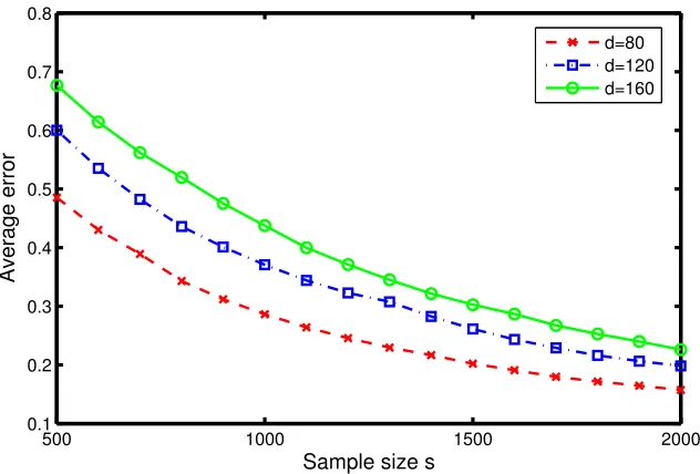
Figure 1: Plot of the average Frobenius error _kMb₋M∗_k2_F/d2 versus the sample size s for three different matrix sizesd_{∈ {}80,120,160_}, all with rankr=2.

dimension)_kMb₋M∗_k2_F/d2 versus a range of sample sizess=_|S_|, with the noise levelσtaken to beα/2, for three different matrix sizes,d_{∈ {}80,120,160_}. Naturally, in each case, the Frobenius error decays assincreases, although larger matrices require larger sample sizes, as reflected by the upward shift of the curves asdis increased.

Next, we compare the performance of the max-norm based regularization with that of the trace-norm using the same criterion as in Davenport et al. (2012). More specifically, the target matrixM∗ is constructed at random by generatingM=LRT, whereLandRared_×rmatrices with i.i.d. entries drawn from Uniform [₋1/2,1/2], so that rank(M∗_{) =r. It is then scaled such thatkM}∗_k∞=1, while in the last case,M∗is formed such that_kM∗kF/d=1. As before, we focus on the Gaussian conditional model but with noise levelσvaries from 10−3 to 10, and setd =500,r=1 ands= 0.15d2, which is exactly the same case studied in Davenport et al. (2012). We plot in Figure 2 the squared Frobenius norm of the error (normalized by the norm of the underlying matrixM∗) over a range of different values of noise levelσon a logarithmic scale. As evident in Figure 2, the max-norm based regularization performs slightly but consistently better than the trace-max-norm, except on the one point whereσ=log₁₀(0.25). Also, we see that for both methods, the performance is poor when the noise is either too little or too much.

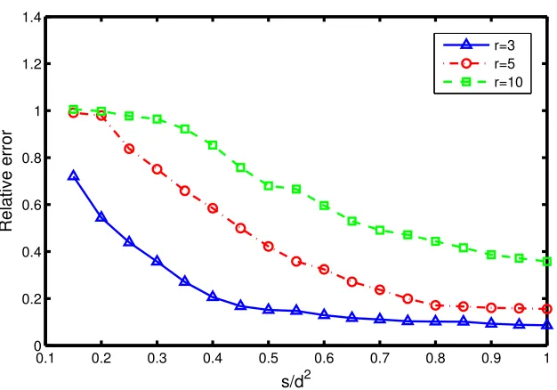
In the third experiment, we consider matrices with dimension d=200 and choose a moderate level of noise, that is, σ=log₁₀(₋0.75), according to previous experiences. Figure 3 plots the relative Frobenius norm of the error versus the sample sizesfor three different matrix ranks,r_∈

-30 -2.5 -2 -1.5 -1 -0.5 0 0.5 1 0.2

0.4 0.6 0.8 1 1.2 1.4

log 10(σ)

Relative error

max-norm

trace-norm

Figure 2: Plot of the relative Frobenius error _kMb₋M∗_k2_F/_kM∗_k2_F versus the noise level σ on a logarithmic scale, with rank r =1, using both max-norm and trace-norm constrained methods.

0.1 0.2 0.3 0.4 0.5 0.6 0.7 0.8 0.9 1

0 0.2 0.4 0.6 0.8 1 1.2 1.4

s/d2

Relative error

r=3 r=5 r=10

6. Discussion

This paper studies the problem of recovering a low-rank matrix based on highly quantized (to a single bit) noisy observation of a subset of entries. The problem was first formulated and analyzed by Davenport et al. (2012), where the authors consider approximately low-rank matrices in terms that the singular values belong to a scaled Schatten-1 ball. When the infinity norm of the unknown matrixM∗ is bounded by a constant and its entries are observed uniformly in random, they show thatM∗can be recovered from binary measurements accurately and efficiently.

Our theory, on the other hand, focuses on approximately low-rank matrices in the sense that unknown matrix belongs to certain max-norm ball. The unit max-norm ball is nearly the convex hull of rank-1 matrices whose entries are bounded in magnitude by 1, thus is a natural convex relaxation of low-rank matrices, particularly with bounded infinity norm. Allowing for non-uniform sampling, we show that the max-norm constrained maximum likelihood estimation is rate-optimal up to a constant factor, and that the corresponding convex program may be solved efficiently in polynomial time. An interesting question naturally arises that whether it is possible to push the theory further to cover exact low-rank matrix completion from noisy binary measurements.

The numerical study in Section 5 provides some evidence of the efficiency of the max-norm constraint approach in 1-bit matrix completion problem. More extensive experimental studies, ap-plications to real data, and numerical comparisons with empirically weighted trace-norm method in a non-uniform scenario will be left as future work.

In our previous work (Cai and Zhou, 2013), we suggest to use max-norm constrained least square estimation to study standard matrix completion (from observations where additive noise is present) under a general sampling model. Similar error bounds are obtained, which are tight to within a constant. Comparing both results in the case of Gaussian noise demonstrates that as long as the signal-to-noise ratio remains constant, almost nothing is lost by quantizing to a single bit.

7. Proofs

We provide the proofs of the main results in this section.

7.1 Proof of Theorem 3

The proof of Theorem 3 is based on general excess risk bounds developed in Bartlett and Mendelson (2002) for empirical risk minimization when the loss function is Lipschitz. We regard matrix recov-ery as a prediction problem, that is, consider a matrixM_∈Rd1×d2 _{as a function: [d1]×[d2]→R,} that is,M(k,l) =Mk,l. Moreover, define a functiong(x;y)R× {±1} 7→R, which can be seen as a loss function:

g(x;y) =1_{y=1}log

1 F(x)

+1_{y=−1}log

1 1₋F(x)

.

For a subsetS=_{(i1,j1), ...,(in,jn)} ⊆([d1]×[d2])n of the observed entries ofY, let

D

S(M;Y) = 1

n∑ n

t=1g(Mit,jt;Yit,jt) = 1

nℓS(M;Y)be the average empirical likelihood function, where the training setSis drawn i.i.d. according toΠ(with replacement) on[d1]_×[d2]. Then we have

D

Π(M;Y):=ES_∼Π[g(Mit,jt;Yit,jt)] =

∑

(k,l)∈[d1]×[d2]

Under condition (U3), we can considergas a function:[₋α,α]_{× {±}1_{} →R}, such that for any y_{∈ {±}1_}fixed,g(_·;y)is essentially anLα-Lipschitz loss function. Also notice that in the current case, Yi,j take ±1 values and appear only in indicator functions, 1{Yi,j =1} and 1{Yi,j =−1}. Therefore, a combination of Theorem 8, (4) of Theorem 12 from Bartlett and Mendelson (2002) as well as the upper bound(6)on the Rademacher complexity of the unit max-norm ball yields that, for anyδ>0, the following inequality holds with probability at least 1₋δover choosing a training setSof 2<n_≤d1d2index pairs according toΠ:

sup M∈Kmax(α,R)

EY

D

Π(M;Y)−EY

D

S(M;Y)

≤17LαR

r

d n+Uα

r

8 log(2/δ)

n :=Rn(α,r;δ). (31)

SinceMbmaxis optimal andM∗is feasible to the optimization problem(13), we have

D

S(Mbmax;Y)≤

D

S(M∗;Y) =

1 n

n

∑

t=1

g(M_i∗_t,jt;Yit,jt).

BecauseM∗has a fixed value which does not depend onS, the empirical likelihood term

D

S(M∗;Y) is an unbiased estimator of

D

Π(M∗;Y), that is,

ES∼Π[

D

S(M∗;Y)] =

D

Π(M∗;Y).

Next, we will derive an upper bound on the deviation

D

S(M∗;Y)−

D

Π(M∗;Y)that holds with high probability. To do this, let A1, ...,An be independent random variables taking values in[d1]×[d2] according to Π, that is, P[At = (k,l)] =πkl,t=1, ...,n, such that

D

S(M∗;Y) = 1_n∑tn=1g(MAt;YAt) and

D

S(M∗;Y)−

D

Π(M∗;Y) =

1 n

n

∑

t=1

g(M_A∗_t;YAt)−E[g(M∗At;YAt)]

.

Then we apply the Hoeffding’s inequality to the random variablesZAt:=g(MA∗t;YAt)−E[g(MA∗t;YAt)], conditionally onY. Observe that 0_≤g(M_A∗_t;YAt)≤Uαalmost surely for all 1≤t≤n, therefore for anyu>0, we have

PS∼Π

D

S(M∗;Y)−

D

Π(M∗;Y)>u ≤exp

−2nu

2 U2

α

, (32)

which in turn implies that that with probability at least 1₋δover choosing a subsetSaccording to

Π,

D

S(M∗;Y)−

D

Π(M∗;Y)≤Uα

r

log(1/δ)

2n . (33)

Putting pieces together, we get

EY

D

Π(Mbmax;Y)−

D

Π(M∗;Y)

= EY

D

Π(Mbmax;Y)−

D

S(M∗;Y)

+EY

D

S(M∗;Y)−

D

Π(M∗;Y)

≤ EY

D

Π(Mmaxb ;Y)−

D

S(Mmaxb ;Y)

+_EY

D

S(M∗;Y)−

D

Π(M∗;Y)

≤ sup

M∈Kmax(α,R)

EY[

D

Π(M;Y)]−EY[

D

S(M;Y)] (34)

+EY

Moreover, observe that the left-hand side of(34)is equal to

EY

D

Π(Mmax;Yb )−

D

Π(M∗;Y)

=

_∑

(k,l)∈[d1]×[d2]

πkl

F(M∗_k,l)log

_F(M∗

k,l) F((Mmax)b k,l)

+ (_F(M¯ ∗ k,l))log

_F(M¯ ∗

k,l) ¯

F((Mmax)b k,l)

,

which is the weighted Kullback-Leibler divergence between matricesF(M)andF(Mmax), denotedb byKΠ(F(M)kF(Mmax)), whereb

¯

F(_·):=1₋F(_·) and F(M):= (F(Mk,l))d1×d2.

This, combined with(31),(33)and(34)imply that for anyδ>0, the following inequality holds with probability at least 1₋δoverS:

KΠ(F(M∗)kF(Mbmax))≤Rn(α,r;δ/2) +Uα

r

log(2/δ)

2n . (35)

Together,(8),(35)and Lemma 8 below establish(16).

Lemma 8 (Lemma 2, Davenport et al., 2012) Let F be an arbitrary differentiable function, and s,t are two real numbers satisfying_|s_|,_|t_{| ≤}α. Then

d_H2(F(s);F(t))_≥ inf |x_|≤α

(F′(x))2

8F(x)(1₋F(x))·(s−t) 2

The proof of Theorem 3 is now completed.

7.2 Proof of Theorem 5

The proof for the lower bound follows an information-theoretic method based on Fano’s inequality (Cover and Thomas, 1991), as used in the proof of Theorem 3 in Davenport et al. (2012). To begin with, we have the following lemma which guarantees the existence of a suitably large packing set forKmax(α,R)in the Frobenius norm. The proof follows from Lemma 3 of Davenport et al. (2012) with a simple modification, see, for example, the proof of Lemma 3.1 in Cai and Zhou (2013).

Lemma 9 Let r= (R/α)2 _{andγ≤1 be such that r≤γ}2_{min(d1,d2) is an integer. There exists a} subset

S

(α,γ)_⊆Kmax(α,R)with cardinality

|

S

(α,γ)_|=

exp

rmax(d1,d2) 16γ2

+1

and with the following properties:

(i) For any N_∈

S

(α,γ),rank(N)_{≤ γ}r2 andNk,l∈ {±γα/2}, such that

kN_k∞=

γα

2 , 1 d1d2kNk

2 F=

γ2_α2

(ii) For any two distinctNk,Nl∈

S

(α,γ),

1 d1d2k

Nk₋Nl_k2_F>γ

2_α2

8 .

Then we construct the packing set

M

by letting

M

=nN+α(1₋γ/2)Ed1,d2:N∈

S

(α,γ)

o

, (36)

where Ed1,d2 ∈R

d1×d2 _{is such that the (d}

1,d2)th entry equals one and others are zero. Clearly,

|

M

|=_|

S

(α,γ)_|. Moreover, for anyM∈

M

,Mk,l∈ {α,(1−γ)α}by the construction of

S

(α,γ)and (36), and

kM_kmax=kN+α(1−γ/2)Ed1,d2kmax≤

α√r

2 +α(1−γ/2)≤α

√

r,

provided thatr_≥4. Therefore,

M

is indeed aδ-packing ofKmax(α,R)in the Frobenius metric with

δ2₌α2γ2d1d2

8 ,

that is, for any two distinctM,M′_∈

M

, we have_kM₋M′_kF ≥δ.

Next, a standard argument (Yang and Barron, 1999; Yu, 1997) yields a lower bound on the

k · kF-risk in terms of the error in a multi-way hypothesis testing problem. More concretely,

inf b

M

max M∈Kmax(α,R)

EkMb₋M_k2_{F ≥}δ

2 4 minMe P

(Me₆=M⋆),

where the random variableM⋆_∈Rd1×d2 _{is uniformly distributed over the packing set}

_M

_{, and the} minimum is carried out over all estimators Me taking values in

M

. Applying Fano’s inequality (Cover and Thomas, 1991) gives the lower bound

P(Me₆=M⋆)_≥1₋I(M

⋆_;Y

S) +log 2

log_|

M

| , (37)

whereI(M⋆;YS)denotes the mutual information between the random parameterM⋆in

M

and the observation matrixYS. Following the proof of Theorem 3 in Davenport et al. (2012), we could bound I(M⋆;YS)as follows:

I(M⋆;YS)≤ max

M,M′_∈M,M6=M′K(YS|MkYS|M

′₎

= max

M,M′_∈M,M6=M′

∑

(k,l)∈S

K(Yk,l|Mk,lkYk,l|Mk′,l)

≤ n[F(α)−F((1−γ)α)]

2 F((1₋γ)α)[1₋F((1₋γ)α)]≤

nα2_γ2

β₍1₋γ)α

,

where the last inequality holds provided thatF′(x)is decreasing on(0,∞). Substituting this into the Fano’s inequality(37)yields

P(Me₆=M⋆)_≥1₋ nα

2_γ2

β₍1₋γ)α

+log 2.r(d1∨d2) 16γ2

Recall thatγ∗_{>0 solves the equation(22):}

γ∗=min

1 2,

R1/2

α

_β

(1₋γ∗_)α(d₁∨d₂)

32n

1/4

.

Requiring

64 log(2)(γ∗)2

d1_∨d2 ≤r≤(d1∧d2)(γ ∗₎2_,

which is guaranteed by(23), to ensure that this probability is least 1/4. Consequently, we have

inf b

M

max M∈Kmax(α,R)

EkMb₋M_k2_{F ≥}α

2_(γ∗)2_d 1d2

128 ,

which in turn implies(24).

7.3 Proof of Theorem 7

The proof of Theorem 7 modifies the proof of Theorem 3, therefore we only summarize the key steps in the following. Let _{A1, ...,An}={(i1,j1), ...,(in,jn)} be independent random variables taking values in[d1]_×[d2]according toΠ, and recall that

ℓS(M;Y) = s

∑

t=1

h

1_{Y

At=1}log

₁

F(MAt)

+1_{Y

At=−1}log

₁

1₋F(MAt)

i

.

According to Srebro et al. (2005) and the proof of Theorem 3, it suffices to derive an upper bound on

∆:=Eh sup

M_∈KΠ,∗

n

∑

t=1

εt

√_π

it·π·jt (Mw)At

i

=Eh sup M∈K∗(α,r)

n

∑

t=1

εt

√_π

it·π·jt MAt

i

,

whereεt are i.i.d. Rademacher random variables. Then it follows from(5)that

∆_≤α√r_·Eh sup

kuk2=kvk2=1

n

∑

t=1

εt

√_π

it·π·jt uitvjt

i

= α√r·E

sup kuk2=kvk2=1

∑

i,j

∑

t:(it,jt)=(i,j)

εt

√_π

it·π·jt

uivj

= α√r_·Eh

n

∑

t=1

εt eite

T jt

√_π

it·π·jt

i.

An upper bound on the above spectral norm has been derived in Foygel et al. (2011) using a

recent result of Tropp (2012). Let Qt =εt e_iteT

jt √_π

it·π·jt ∈R

d1×d2 _{be i.i.d. random matrices with}

zero-mean, then the problem reduces to estimate_Ek∑st=1Qtk. Following the the proof of Foygel et al. (2011), we see that, under condition(26)

E n

∑

t=1

Qt

≤Cσ1

p

log(d) +σ2log(d)

with

σ1 = n·max

max k

∑

_l

πkl

πk·π·l

,max l

∑

_k

πkl

πk·π·l

≤µnmax_{d1,d2_},

σ2 = max

k,l 1

√_π

k_·π_·l ≤

µpd1d2.

Putting above estimates together, we conclude that

∆_≤Cα√rpµnmax_{d1,d2}log(d) +µ

p

d1d2log(d)

,

which in turn yields that for anyδ_∈(0,1), inequality

KΠ(F(M∗)kF(Mbw,tr))

≤ C

Lαα

r

µrmax_{d1,d2}log(d)

n +Uα

r

log(4/δ) n

holds with probability at least 1₋δ, provided thatn_≥µmin_{d1,d2_}log(d).

7.4 An Extension to Sampling Without Replacement

In this paper, we have focused on sampling with replacement. We shall show here that in the uniform sampling setting, the results obtained in this paper continue to hold if the (binary) entries are sampled without replacement. Recall that in the proof of Theorem 3, we letA1, ...,Anbe random variables taking values in[d1]×[d2],S={A1, ...,An}and assume theAt’s are distributed uniformly and independently, that is, S_∼Π=_{πkl} withπkl ≡ _d11_d2. The purpose now is to prove that the arguments remain valid when theAt’s are selected without replacement, denoted byS∼Π0. In this notation, we have

D

S=

1 n_(i,

∑

_j)

∈S

g(Mi,j;Yi,j) and

D

Π0=ES∼Π0[

D

S] = 1 d1d2₍

∑

_k,l)

g(Mk,l;Yk,l).

By Lemma 3 in Foygel and Srebro (2011) and(31), for anyδ>0,

sup M∈Kmax(α,R)

EY

D

Π0(M;Y)−EY

D

S(M;Y)

≤17LαR

r

d n+Uα

r

8(log(4n) +log(2/δ)) n

Eexp(λSX). According to the notion of negative association (Joag-Dev and Proschan, 1983), it is well-known thatmY(λ) =Eexp(λSY)≤mX(λ), which in turn gives a similar large deviation bound forSY. Therefore, inequalities(32)and(33)are still valid if Πis replaced byΠ0. Keep all other arguments the same, we get the desired result.

Acknowledgments

The authors would like to thank Yaniv Plan for helpful discussions and for pointing out the impor-tance of allowing non-uniform sampling. We also thank the Associate Editor and two referees for thorough and useful comments which have helped to improve the presentation of the paper. The research of Tony Cai was supported in part by NSF FRG Grant 0854973, NSF Grant DMS-1208982, and NIH Grant R01 CA127334. A part of this work was done when the second author was visiting the Wharton Statistics Department of the University of Pennsylvania. He wishes to thank the institution and particularly Tony Cai for their hospitality.

References

A. Ai, A. Lapanowski, Y. Plan and R. Vershynin. One-bit compressed sensing with non-Gaussian measurements. Linear Algebra and Its Applications, forthcoming, 2013.

P. Bartlett and S. Mendelson. Rademacher and Gaussian complexities: risk bounds and structural results. Journal of Machine Learning Research,3:463–482, 2002.

P. Biswas, T. C. Lian, T. C. Wang and Y. Ye. Semidefinite programming based algorithms for sensor network localization. ACM Transactions on Sensor Networks,2(2):188–220, 2006.

P. Boufounos and R. G. Baraniuk. 1-bit compressive sensing. InProceedings of the 42nd Annual Conference on Information Sciences and Systems, pages 16–21, Princeton, NJ, March 2008.

S. Burer and R. D. C. Monteiro. A nonlinear programming algorithm for solving semidefinite pro-grams via low-rank factorization. Mathematical Programming, Series B,95(2):329–357, Febru-ary 2003.

T. T. Cai and W.-X. Zhou Matrix completion via max-norm constrained optimization.arXiv preprint arXiv:1303.0341, 2013.

T. M. Cover and J. A. Thomas. Elements of Information Theory. John Wiley and Sons, New York, 1991.

M. A. Davenport, Y. Plan, E. van den Berg and M. Wooters. 1-bit matrix completion.arXiv preprint arXiv:1209.3672, 2012.

R. Foygel, R. Salakhuidinov, O. Shamir and N. Srebro. Learning with the weighted trace-norm un-der arbitrary sampling distributions. Advances in Neural Information Processing Systems (NIPS), 24, pages 2133–2141, 2011.