On the Behavior of Intrinsically High-Dimensional Spaces:
Distances, Direct and Reverse Nearest Neighbors, and
Hubness
Fabrizio Angiulli [email protected]
DIMES – Dept. of Computer, Modeling, Electronics, and Systems Engineering University of Calabria
87036 Rende (CS), Italy
Editor:Sanjiv Kumar
Abstract
Over the years, different characterizations of the curse of dimensionality have been pro-vided, usually stating the conditions under which, in the limit of the infinite dimensionality, distances become indistinguishable. However, these characterizations almost never address the form of associated distributions in the finite, although high-dimensional, case. This work aims to contribute in this respect by investigating the distribution of distances, and of direct and reverse nearest neighbors, in intrinsically high-dimensional spaces. Indeed, we derive a closed form for the distribution of distances from a given point, for the expected distance from a given point to itskth nearest neighbor, and for the expected size of the ap-proximate set of neighbors of a given point in finite high-dimensional spaces. Additionally, the hubness problem is considered, which is related to the form of the function Nk repre-senting the number of points that have a given point as one of their knearest neighbors, which is also called the number ofk-occurrences. Despite the extensive use of this function, the precise characterization of its form is a longstanding problem. We derive a closed form for the number of k-occurrences associated with a given point in finite high-dimensional spaces, together with the associated limiting probability distribution. By investigating the relationships with the hubness phenomenon emerging in network science, we find that the distribution of node (in-)degrees of some real-life, large-scale networks has connections with the distribution ofk-occurrences described herein.
Keywords: high-dimensional data, distance concentration, distribution of distances, nearest neighbors, reverse nearest neighbors, hubness
1. Introduction
Although the size and the dimensionality of collected data are steadily growing, traditional techniques usually slow down exponentially with the number of attributes to be considered and are often overcome by linear scans of the whole data. In particular, the term curse of dimensionality (Bellmann, 1961), is used to refer to difficulties arising whenever high-dimensional data has to be taken into account.
One of the main aspects of this curse is known as distance concentration (Demartines, 1994), which is the tendency for distances to become almost indiscernible in high-dimensional spaces. This phenomenon may greatly affect the quality and performances of machine learn-ing, data minlearn-ing, and information-retrieval techniques. This effect results because almost
c
all these techniques rely on the concept of distance, or dissimilarity, among data items in order to retrieve or analyze information. However, whereas low-dimensional spaces show good agreement between geometric proximity and the notion of similarity, as dimensional-ity increases, different counterintuitive phenomena arise that may be harmful to traditional techniques.
Over time, different characterizations of the curse of dimensionality and related phe-nomena have been provided (Demartines, 1994; Beyer et al., 1999; Aggarwal et al., 2001; Hinneburg et al., 2000; Fran¸cois et al., 2007). These characterizations usually state con-ditions under which, according to the limits of infinite dimensionality, distances become indistinguishable. However, almost never do these conditions address the form of associ-ated distributions in finite, albeit high-dimensional, cases.
This work aims to contribute in this area by investigating the distribution of distances and of some related measures in intrinsically high-dimensional data. In particular, the analysis is conducted by applying the central limit theorem to the Euclidean distance ran-dom variable to approximate the distance probability distribution between pairs of ranran-dom vectors, between a random vector and realizations of a random vector, and to obtain the expected distance from a given point to itskth nearest neighbor. It is then shown that an understanding of these distributions can be exploited to gain knowledge of the behavior of high-dimensional spaces, specifically the number of approximate nearest neighbors and the number of reverse nearest neighbors that are also investigated herein.
Nearest neighbors are transversal to many disciplines (Preparata and Shamos, 1985; Dasarathy, 1990; Beyer et al., 1999; Duda et al., 2000; Ch´avez et al., 2001; Shakhnarovich et al., 2006). In order to try to overcome the difficulty of answering nearest neighbor queries in high-dimensional spaces (Weber et al., 1998; Beyer et al., 1999; Pestov, 2000; Giannella, 2009; Kab´an, 2012), the concept of the-approximate nearest neighbor (Indyk and Motwani, 1998; Arya et al., 1998) has been introduced. The -neighborhood of a query point is the set of points located at a distance not greater than (1 +) times the distance separating the query from its true nearest neighbor.
Related to the notion of the -approximate nearest neighbor is the notion of neigh-borhood or query instability (Beyer et al., 1999): a query is said to be unstable if the -neighborhood of the query point consists of most of the data points. Although asymptotic results, such as that reported by Beyer et al. (1999), tell what happens when dimensionality is taken to infinity, nothing is said about the dimensionality at which the nearest neigh-bors become unstable. Pursuant to this scenario, this paper derives a closed form for the expected size of the-neighborhood in finite high-dimensional spaces, an expression that is then exploited to determine the critical dimensionality. Also, to quantify the difficulty of (approximate) nearest neighbor search, He et al. (2012) introduced the concept of relative contrast, a measure of separability of the nearest neighbor of the query point from the rest of the data, and provided an estimate which is applicable for finite dimensions. By leveraging the results concerning distance distributions, this paper derives a more accurate estimate for the relative contrast measure.
Muthukrishnan, 2000; Singh et al., 2003; Tao et al., 2007; Cheong et al., 2011; Yang et al., 2015), with uses having been proposed in the data mining and machine learning fields (Williams et al., 2002; Hautam¨aki et al., 2004; Radovanovic et al., 2009, 2010; Tomasev et al., 2014; Radovanovic et al., 2015; Tomasev and Buza, 2015), beyond being the objects of study in applied probability and mathematical psychology (Newman et al., 1983; Maloney, 1983; Tversky et al., 1983; Newman and Rinott, 1985; Yao and Simons, 1996).
Despite the usefulness and the extensive use of this construct, the precise characteri-zation of the form of the function Nk both in the finite and infinite dimensional cases is a longstanding problem. What is already known is that for the infinite limit of size and dimension, Nk must converge in its distribution to zero; however, this result and its inter-pretations seem to be insufficient to characterize its observed behavior in finite samples and dimensions. Consequently, this paper derives a closed form of the number ofk-occurrences associated with a given point in finite high-dimensional spaces, together with a generalized closed form of the associated limiting probability distribution that encompasses previous results and provides interpretability of its behavior and of the related hubness phenomenon. The results, which are first illustrated for independent and identically distributed data, are subsequently extended to independent non-identically distributed data satisfying certain conditions, and then, connections with non-independent real data are depicted. Finally, it is discussed how to potentially extend the approach to Minkowski’s metrics and, more generally, to distances satisfying certain conditions of spatial centrality.
Because hubness is a phenomenon of primary importance in network science, we also investigate if the findings relative to the distribution of the reverse nearest neighbors and the emergence of hubs in intrinsically high-dimensional contexts is connected to an analogous phenomenon occurring in the context of networks. The investigation reveals that for some real-life large-scale networks, the distribution of the incoming node degrees is connected to the herein-derived distribution of the infinite-dimensional k-occurrences function, which models the number of reverse k-nearest neighbors in an arbitrarily large feature space of independent dimensions. Hence, the provided distribution also appears to be suitable for modelling node-degree distributions in complex real networks.
The current study can be leveraged in several ways and in different contexts, such as in direct and reverse nearest neighbor searches, density estimation, anomaly and novelty detection, density-based clustering, and network analysis, among others. With regard to its possible applications, we can highlight approximations of measures related to distance distributions, worst-case scenarios for data analysis and retrieval techniques, design strate-gies that try to mitigate the curse of dimensionality, and models of complex networks. We refer to the concluding section for a more extensive discussion.
2. Related Work
As already noted, the term curse of dimensionality is used to refer to difficulties arising when high-dimensional data must be taken into account, and one of the main aspects of this curse is distance concentration. In this regard, Demartines (1994) has shown that the expectation of the Euclidean norm of independent and identically distributed (i.i.d.) random vectors increases as the square root of the dimension, whereas its variance tends toward a constant and, hence, does not depend on the dimensionality. Specifically:
Theorem 1 (Demartines, 1994, cf. Theorem 2.1) Let Xd be an i.i.d. d-dimensional
random vector with common cdf FX. Then
E[kXdk2] =
√
ad−b+O(1/d) and σ2(kX
dk2) =b+O(1/
√ d),
where aand bare constants depending on the central moments ofFX up to the fourth order
but do not depend on the dimensionality d.
Demartines noticed that, because the Euclidean distance corresponds to the norm of the difference of two vectors, the distance between the i.i.d. random vectors must also exhibit the same behavior. This insightful result explains why high-dimensional vectors appear to be distributed around the surface of a sphere of radiusE[kXdk] and why, because they seem to be normalized, the distances between pairs of high-dimensional random vectors tend to be similar.
The distance concentration phenomenon is usually characterized in the literature by means of a ratio between some measure related to the spread and some measure related to the magnitude of the norm, sometimes presented as the distance from a point located in the origin of the space. In particular, the conclusion is that there is a concentration of distances when the above ratio converges to 0 as the dimensionality tends to infinity.
Some authors have studied the concentration phenomenon by representing a data set as a set of n d-dimensional i.i.d. random vectors X(dj) (1 ≤ j ≤ n) with not-necessarily common pdfsfX(j). Specifically, thecontrast is defined as the difference between the largest
and the smallest observed norm, or rather the distance from a query point located at the origin, whereas therelative contrast is defined as
RCd=
maxjkX(dj)kp−minjkX(dj)kp minjkX(dj)kp
,
where k · kp denotes the p-normkxdkp =
Pd
i=1|xi|p
1/p
, is the contrast normalized with respect to the smallest norm/distance.
Theorem 2 (Adapted from Beyer et al., 1999, cf. Theorem 1)LetX(dj)(1≤j ≤n)
be n d-dimensional random vectors with common cdfs. If
lim d→∞σ
2 kX (j) d kp E[kX(dj)kp]
!
= 0, then, for any >0, lim
If the hypothesis is verified, that is, if the variance of the ratio between the norm of the vectors and their expected value vanishes as the dimensionality goes to infinity, then the relative contrast also becomes smaller and smaller, and all the vectors seem to be located at approximatively the same distance from the reference vector. That is, given a query point Qd, the distance from the nearest and the furthest neighbor become negligible:
lim d→∞P r
max
j kQd−X (j)
d kp ≤(1 +) minj kQd−X (j) d kp
= 1.
In (Beyer et al., 1999), it is shown that i.i.d. random vectors satisfy the above condition. Other authors have provided characterizations of the concentration phenomenon by providing upper and lower bounds to the relative contrast in the cases of Minkowski and fractional norms (Hinneburg et al., 2000; Aggarwal et al., 2001).
Subsequently, (Fran¸cois et al., 2007) posed the following problem: is the concentration phenomenon a side effect of theEmpty Space Phenomenon (Bellmann, 1961), just because we consider a finite number of points in a bounded portion of a high-dimensional space? To explore this problem, they studied the concentration phenomenon by taking the same perspective as Demartines, i.e., to refer to a distribution rather than to a finite set of points. The relative variance
RVd=
σ(kXdkp) E[kXdkp]
is a measure of concentration for distributions, corresponding to the ratio between the standard deviation and the expected value of the norm.
Theorem 3 (Adapted from Fran¸cois et al., 2007, cf. Theorem 5) Let Xd be an
i.i.d. d-dimensional random vector. Then
lim
d→∞RVd= 0.
From the above result, they conclude that the concentration of the norms in high-dimensional spaces is an intrinsic property of the norms and not a side effect of the finite sample size or of the Empty Space Phenomenon. Because it does not depend on the sample size, this can be regarded as an extension of Demartines’ results to allp-norms.
As a consequence of the distance concentration, the separation between the nearest neighbor and the farthest neighbor of a given point tend to become increasingly indistinct as the dimensionality increases.
Related to the analysis of i.i.d. data is the concept of intrinsic dimensionality. Although variables used to identify each datum could not be statistically independent, ultimately, the intrinsic dimensionality of the data is identified as the minimum number of variables needed to represent the data itself (van der Maaten et al., 2009). This corresponds in linear spaces to the number of linearly independent vectors needed to describe each point. As a matter of fact, an extensively used notion of intrinsic dimensionality, the correlation dimension
(Grassberger and Procaccia, 1983), is based on identifying the dimensionality D at which the Euclidean space is homeomorphic to the manifold containing the support of the data:
D= lim δ→0
where Fdst denotes the cumulative distribution function of pairwise distances, which for-malizes the notion that in the limit of small length-scales (δ→0) upon which the manifold the data lie, the manifold is homeomorphic to the Euclidean space of dimension D.
And, indeed, (Demartines, 1994) mentions that if random vector components are not independent, the concentration phenomenon is still present provided that the actual number
Dof “degrees of freedom” is sufficiently large. Thus, results derived for i.i.d. data continue to be valid provided that the dimensionalitydis replaced withD. Moreover, (Beyer et al., 1999) provided different examples of data presenting concentration, all of which share with the i.i.d. case a sparse correlation structure. (Durrant and Kab´an, 2009) noted that it is difficult to identify meaningful workloads that do not exhibit concentration, and showed that for the family of linear latent variable models, a class of data distributions having non-i.i.d. dimensions, the Euclidean distance will not become concentrated as long as the number of relevant dimensions grows no more slowly than the overall data dimensions do. This also confirms that weakly dependent data lead to concentration; however, they also noted that the condition to avoid concentration is not often met in practice.
Another aspect of the curse of dimensionality problem, closely related to the distance concentration and the nearest neighbor relationship, is the so called hubness phenomenon. This phenomenon has been previously observed in several applications (Doddington et al., 1998; Singh et al., 2003; Aucouturier and Pachet, 2007), has recently undergone to direct investigation (Radovanovic et al., 2009, 2010; Low et al., 2013), and has been subjected to several different proposed techniques for overcoming the phenomenon (Radovanovic et al., 2015; Tomasev, 2015).
Specifically, consider the number Nk(xd) of observed points that havexdamong theirk nearest neighbors. Nk is also called k-occurrences or the reversek-nearest neighbor count.
It is known that in low dimensional spaces, the distribution of Nk complies with the binomial one and, in particular, for uniformly distributed data in low dimensions, it can be modeled as node in-degrees in the k-nearest neighbor graph, which follows the Erd˝ os-R´enyi random graph model, with a binomial degree distribution (Erd˝os and R´enyi, 1959). However, it has been observed that as dimensionality increases, the distribution of Nk becomes skewed to the right, resulting in the emergence of hubs, which are points whose reversek-nearest neighbor counts tend to be meaningfully larger than that associated with any other point.
The distribution of Nkhas been explicitly studied in the applied probability and mathe-matical psychology communities (Newman et al., 1983; Maloney, 1983; Newman and Rinott, 1985; Tversky and Hutchinson, 1986; Yao and Simons, 1996). Almost all the results pro-vided concern a Poisson process that spreads the vectors uniformly over Rd, leading to
the conclusion that the limiting distribution of Nk converges to the Poisson distribution with mean k. The case of continuous distributions with i.i.d. components has been con-sidered in (Newman et al., 1983; Newman and Rinott, 1985), where the expression for the infinite-dimensional distribution of N1 is characterized as follows.
Theorem 4 (Newman et al., 1983, cf. Theorem 7) Let {X(0)d , X(1)d , . . ., X(dn)} be i.i.d. random vectors with a common continuous cdf having a finite fourth moment. Let
respect to the Euclidean distance is X(0)d . Then
lim
n→∞dlim→∞N n,d 1
D
−→0 and lim
n→∞dlim→∞σ 2(Nn,d
1 ) =∞.
The interpretation of the above result due to (Tversky et al., 1983) is that if the number of dimensions is large relative to the number of points, a large portion of points will have reverse nearest neighbor count equaling zero, whereas a small fraction (i.e., the hubs) will score large counts.
In order to provide an explanation for hubness, (Radovanovic et al., 2010) noticed that it is expected for points that are closer to the mean of the data distribution to be closer, on average, to all other points. However, empirical evidence indicates that this tendency is amplified by high-dimensionality, making points that reside in the proximity of the datas mean become closer to all other points than their low-dimensional analogues are. This tendency causes high-dimensional points that are closer to the mean to have increased probability of being selected as k-nearest neighbors by other points, even for small values of k.
In order to formalize the above evidence in finite-dimensional spaces, the authors con-sidered the simplified setting of normally distributed i.i.d. d-dimensional random vectors, for which the distribution of Euclidean distances, which are calculated as the square root of the sum of squares of i.i.d. normal variables, corresponds to a chi distribution with d
degrees of freedom (Johnson et al., 1994) and the random variable kxd−Ydk, represent-ing the distance from a fixed point xd to the rest of the data, follows the noncentral chi distribution withddegrees of freedom and noncentrality parameter λ=kxdk(Oberto and Pennecchi, 2006).
Theorem 5 (Radovanovic et al., 2010, cf. Theorem 1) Let λd,1 = µχ(d)+c1σχ(d)
and λd,2 = µχ(d) +c2σχ(d), where d ∈ N+, c1 < c2 ≤ 0, and µχ(d) and σχ(d) are the
mean and standard deviation of the chi distribution with ddegrees of freedom, respectively. Define ∆µd(xd,1,xd,2) =µχ(d,λd,2)−µχ(d,λd,1), where µχ(d,λ) is the mean of the noncentral chi distribution withddegrees of freedom and noncentrality parameterλ. Then, there exists
d0 ∈ N such that for every d > d0, ∆µd(λd,1, λd,2) > 0, and ∆µd+2(λd+2,1, λd+2,2) > ∆µd(λd,1, λd,2).
Intuitively, λd,1 and λd,2 represent two d-dimensional points whose norms are located atc1 andc2, resp., standard deviations from the expected value of the norm in the dimen-sionalityd, and for which ∆µd(λd,1, λd,2) is the distance between the expected value of the associated distribution of distances.
3. Notation
In the rest of this section, upper case letters, such asX,Y,Z,. . ., denote random variables (r.v.) taking values in R. fX (FX, resp.) denotes the probability density function (pdf) (probability distribution function (cdf), resp.) associated withX.
Boldface uppercase letters with d as a subscript, such as Xd, Yd, Zd, . . ., denote d -dimensional random vectors taking values in Rd. The components Xi (1 ≤ i ≤ d) of a random vector Xd = (X1, X2, . . . , Xd) are random variables having pdfs fXi = fi (cdf FXi = Fi). A d-dimensional random vector is said to be independent and identically
distributed (i.i.d. for short) if its random variables are independent and have common pdf
fX =fXi (cdf FX =FXi).
Boldface lowercase letters withdas a subscript, such asxd,yd,zd,. . ., denote a specific
d-dimensional vector taking value inRd. The components of a vector xd= (x1, x2, . . . , xd), denoted as xi (1≤i≤d), are real scalar values.
Given a random variable X, w.l.o.g. and for simplicity of treatment, sometimes it is assumed that the expected valueµ(orµX) offX isµ= 0. If that is not the case, to satisfy the assumption, it suffices to replace during the analysis the original random variable X
with the novel random variable ˆX=X−µX. Thus,Xˆddenotes the random vectorXd−µX.
σX orσ(X) (orσ alone, wheneverXis clear from the context) is the standard deviation of the random variableX. Byµk (ˆµk, resp.), orµX,k (ˆµX,k, resp.) wheneverX is not clear from the context, it is denoted the k-th moment (k-th central moment, resp.) (k > 0)
µk = E[Xk] (ˆµk = E[(X−µX)k], resp.) of the random variable X, where E[X] is the expectation of X. Clearly, whenµ=µ1= 0, µk coincides with ˆµk and µ2 =σ2.
Moments of a pdff (cdfF, resp.) are those associated with a random variableXhaving pdf fX = f (cdf FX = f, resp.). The moments of an i.i.d. random vector Xd are those associated with its cdf FX.
It is said that a distribution function has finite (central) moment µk, if there exists 0≤µtop<∞such that |µk| ≤µtop.
Whenever moments are employed during the proofs, we always assume that they exist and are finite. Moreover, if the random variable associated with a moment employed in a proof is not explicitly stated, we assume that the moment is relative to the common cdf of the random vector(s) occurring in the distribution reported in the statement of the theorem. Moreover, it is sometimes considered the case that µ3 = 0, a condition that is referred to as null skewness. It is known that odd central moments, provided they exist, are null if the pdf ofX is symmetric with respect to the mean (with examples of distributions having nullµ3 value being the Uniform and Normal distributions).
The notation N µ, σ2
represents the Normal distribution function with mean µ and variance σ2. By Φ (φ, resp.) one denotes the cdf (pdf, resp.) of the standard normal distribution, whereas by ΦX (φX, resp.) one denotes the cdf (pdf, resp.) of the normal distribution with meanµX and varianceσ2X.
Let X represent a univariate random variable that is defined in terms of a real-valued function of one or more d-dimensional random vectors. For example, X could be defined askXdk2. The notationX' N µX, σX2
is shorthand to denote the fact that, as d→ ∞, the distributionFbX of the standard score X
−µX
N(0,1). Thus, for large values of d, N(µX, σ2X) approximates the distribution probability
FX of X, andP r[X≤δ]≈Φ
δ−µX
σX
.
In the following,k · kdenotes theL2 norm, i.e.,kxdk=
q
Pd
i=1x2i. Moreover, dist(P, Q) denotes the Euclidean distancekP−Qkbetween (random) vector P and (random) vector
Q.
Let x∈R, and letX be a random variable. Then
zx,X =
x−µX
σX
represents the valuexstandardized with respect to the mean and the standard deviation of
X. For ad-dimensional vectorxd, which is the realization of a d-dimensional i.i.d. random vectorYd, the notationzxd is used as shorthand forzkxdk2,kYdk2, i.e.,
zxd =zkxdk2,kYdk2 =
kxdk2−µkYdk2 σkYdk2
.
Results in the following are derived by considering distributions. However, these results can be applied to a finite set of points by taking into account large samples. In order to deal with a finite set of points, {Yd}ndenotes a set of nrandom vectors {Y(1)d , . . . ,Y(dn)}, each one distributed as Yd.
Now we recall the Lyapunov Central Limit Theorem (CLT) condition. Consider the sequenceW1, W2, W3, . . .of independent, but not identically distributed, random variables, and let Vd=
Pd
i=1Wi. By the Lyapunov CLT condition (Ash and Dol´eans-Dade, 1999), if for someδ >0 it holds that
lim d→∞
1
s2+d δ
d
X
i=1 E
h
|Wi−E[Wi]|2+δ
i
= 0, where s2d= d
X
i=1
σW2i, (1)
then, as dgoes to infinity,
Ud−E[Ud]
σ(Ud) =
Pd
i=1Wi−Pdi=1E[Wi]
q
Pd
i=1σ2Wi
→ N(0,1),
i.e., the standard score (Vd−E[Vd])/σ(Vd) converges in distribution to a standard normal random variable.
In the following, when a statement involves a d-dimensional vector xd, we will usually assume that xdis the realization of a specificd-dimensional random vectorXd. Moreover, we will say that a result involving the realizationxd of a random vectorXd holdswith high
probability if the statement is true for all the realizations of Xd except for a subset which becomes increasingly less probable as the dimensionality dincreases.
4. Results
This section presents the results of the work concerning distribution of distances, nearest neighbors, and reverse nearest neighbors.
Specifically, Section 4.1, concerning the distribution of distances between intrinsically high-dimensional data, derives the expressions for the distance distribution between pairs of random vectors and between a realization of a random vector and a random vector, and analyzes the error associated with expressions.
Section 4.2 takes into account the distribution of distances from nearest neighbors, derives the expected size of the -neighborhood in high-dimensional spaces, and leverages it to characterize neighborhood instability. The section also derives a novel estimate of the relative contrast measure.
Section 4.3 addresses the problem of determining the number of k-occurrences and de-termines the closed form of its limiting distribution, showing that it encompasses previous results and provides interpretability of the associated hubness phenomenon.
Section 4.4 generalizes the results derived for the i.i.d. case to independent non-identically distributed data, depicting connections with the behavior in real data.
Section 4.5 discusses relationship to other distances, including Minkowski’s metrics and, in general, distances satisfying certain conditions of spatial centrality.
The first three sections deal with i.i.d. random vectors. In these sections, the synthetic data sets considered consist of data generated from a uniform distribution in [−0.5,+0.5], a standard normal distribution, and an exponential distribution with mean 1.
For the proofs that are not reported within the main text, the reader is referred to the Appendix.
4.1 On the Distribution of Distances for i.i.d. Data
First of all, the probability that two d-dimensional i.i.d. random vectors lie at a distance not greater than δ from one another is considered. The expression of Theorem 6 results from the fact that the distribution of the random variable kXd−Ydk2 converges towards the normal distribution for large dimensionalities.
Theorem 6 Let Xd andYd be twod-dimensional i.i.d. random vectors with common cdf
F. Then, for large values of d,
P r[dist(Xd,Yd)≤δ]≈Φ
δ2−2d(µ 2−µ2)
r
2dµ4+µ22+ 2µ µ(2µ2−µ2)−2µ3
.
Proof of Theorem 6. The statement follows from the property shown in Lemma 7.
Lemma 7 kXd−Ydk2 ' N 2d(µ2−µ2), 2d µ4+µ22+ 2µ µ(2µ2−µ2)−2µ3
.
Proof of Lemma 7. The squared norm kXd−Ydk2 can be written askXd−Ydk2 =
variables
kYdk2 = d
X
i=1
Y2
i and hXd,Ydi= d
X
i=1
XiYi.
The proof proceeds by showing that, as d → ∞, kXdk2, kYdk2, and hXd,Ydi are both normally distributed and jointly normally distributed and by determining their covariance, which is accounted for in Propositions 8, 9, 10, and 11, as reported in the following.
Proposition 8 kYdk2 ' N dµ2, d(µ4−µ22)
.
Proof of Proposition 8. Consider the random variable
kYdk2 = d
X
i=1
Yi2 = d
X
i=1
Wi,
where Wi = Yi2 is a novel random variable. Then, µW = E[Wi] = E[Yi2] = µ2, and
σ2
W =E[Wi2]−E[Wi]2 =E[Yi4]−µ22 =µ4−µ22.
Consider the sequence W1, W2, W3, . . . of i.i.d. random variables. By the Central Limit Theorem (CLT for short) (Ash and Dol´eans-Dade, 1999), the standard score of Wi is such that, asd→ ∞,
Pd
i=1√Wi−dµW
dσW
=
Pd
i=1Yi2−dµ2
p
d(µ4−µ22)
→ N(0,1),
from which the result follows.
Proposition 9 hXd,Ydi ' N dµ2, d(µ22−µ4)
.
Proof of Proposition 9. Because hXd,Ydi = Pdi=1XiYi = Pdi=1Wi is the sum of a sequence W1, W2, W3, . . . of i.i.d. random variables with mean E[Wi] = E[XiYi] = E[Xi]E[Yi] =µ2and varianceσ2[Wi] =E[Wi2]−E[Wi]2=E[Xi2Yi2]−(µ2)2 =E[Xi2]E[Yi2]−
µ4 =µ2
2−µ4, from the CLT the result follows.
Proposition 10 Asd→ ∞,kXdk2, kYdk2 andhXd,Ydi are jointly normally distributed. Proof of Proposition 10. The statement holds provided that all linear combinations
W =akXdk2+bkYdk2+chXd,Ydi are normal. Notice that
W =a
d
X
i=1
Xi2
!
+b
d
X
i=1
Yi2
!
+c
d
X
i=1
XiYi
!
= d
X
i=1
aXi2+bYi2+cXiYi
= d
X
i=1
Wi,
Proposition 11
cov kYdk2,hXd,Ydi
=dµ(µ3−µ2µ)
andcov kXdk2,hXd,Ydi
=dµ(µ3−µ2µ), for symmetry
.
Proof of Proposition 11. See the appendix.
Proof of Lemma 7 (continued). Because the random variables kXdk2, kYdk2, and
hXd,Ydi are jointly normally distributed (see Proposition 10), their linear combination
kXd−Ydk2 =kXdk2+kYdk2−2hXd,Ydiis normally distributed with meanµkXd−Ydk2 = µkXdk2 +µkYdk2−2µhXd,Ydi= 2d(µ2−µ
2), and variance
σ2
kXd−Ydk2 = 2σ
2
kYdk2+ (−2)
2σ2
hXd,Ydi+ 4(−2)cov(kYdk
2,hX
d,Ydi) = = 2d(µ4−µ22) + 4d(µ22−µ4)−8dµ(µ3−µ2µ) =
= 2dµ4+µ22+ 2µ µ(2µ2−µ2)−2µ3
.
Proof of Theorem 6 (continued). To conclude the proof: P r[dist(Xd,Yd)≤δ] =
P r
dist(Xd,Yd)2 ≤δ2
=P r
kXd−Ydk2≤δ2
≈ΦkXd−Ydk2(δ
2).
Note that, if Xd and Yd have a common pdf with null mean (µ= 0), kYdk2 (kXdk2 equivalently) andhXd,Ydiare uncorrelated, and being jointly normal distributed, they are also independent. In such a case, the parameters of the distribution can be expressed in the following simplified form.
Corollary 12 Let Xd and Yd be two d-dimensional i.i.d. random vectors with common
cdf FX having mean µ. Then
kXˆd−Yˆdk2' N 2dµˆ2, 2d(ˆµ4+ ˆµ22)
,
where Xˆd =Xd−µ (Yˆd =Yd−µ, resp.) and µˆk =E[(X−µ)k] (k >0) are the central
moments of fX (the moments of fXˆ, resp.).
Proof of Corollary 12. Immediate from Theorem 7.
The notability of the above expression also stems from the following fact.
Proposition 13 P r[dist(Xd,Yd)≤δ] =P r[dist(Xˆd,Yˆd)≤δ].
Proof of Proposition 13. Distances are not affected by translation.
Corollary 14 Let Xd and Yd be two d-dimensional i.i.d. random vectors with cdfs FX
and FY, respectively. Then kXd−Ydk2 ' N(µX,Y, σX,Y2 ), where
µX,Y = d(µX,2+µY,2−2µXµY), and
σ2
X,Y = d (µX,4−µ2X,2) + (µY,4−µ2Y,2) + 4µX,2µY,2+ 4µXµY µX,2+µY,2−µXµY
+
−4µXµY,3−4µYµX,3
.
Proof of Corollary 14. The expression can be obtained by following the same line of reasoning of Theorem 7.
To characterize more precisely distance distributions, it is of interest to consider the case in which one of the two vectors is held fixed. With this aim, the following Theorem 15 concerns the probability that a given d-dimensional vector xd and the realization of a
d-dimensional i.i.d. random vectorYdlie at a distance not greater thanδfrom one another. The result holds under the condition thatxditself is the realization of ad-dimensional i.i.d. random vectorXd, with the cdf FX ofXd not necessarily being identical to the cdf FY of
Yd.
Formally, Theorem 15 holds with high probability because it relies on a proof of con-vergence in probability exploited in Proposition 17. Although not all the realizations may comply with the condition of Proposition 17 (e.g., consider the casexi =ci withc6= 1), it holds anyway for almost all the realizations, except for a set of vanishing measure.
Theorem 15 Let xd denote a realization of a d-dimensional i.i.d. random vector Xd, and
let Yd be a d-dimensional i.i.d. random vector. Then, for large values of d, with high
probability
P r[dist(xd,Yd)≤δ]≈Φ
δ2− kx
dk2−dµ2+ 2µPdi=1xi
q
d(µ4−µ22) + 4(µ2−µ2)kxdk2−4(µ3−µµ2)Pdi=1xi
,
where moments are relative to the random vector Yd.
Proof of Theorem 15. The proof relies on the result of Lemma 16 considering the distribution of kxd−Ydk2.
Lemma 16 With high probability
kxd−Ydk2' N kxdk2+dµ2−2µ
d
X
i=1
xi, d(µ4−µ22) + 4(µ2−µ2)kxdk2−4(µ3−µµ2)
d
X
i=1
xi
! .
Proposition 17 LetXdbe ad-dimensional i.i.d. random vector having cdfFX. Moreover,
letpandq be positive integers, andβ0, β1, . . . , βp,α0, α1, . . . , αqbe real coefficients such that
βp 6= 0 and αq6= 0. Then, for any >0,
lim d→∞P r
Pd i=1 Pp
j=0βjX j i Pd i=1 Pq
j=0αjX j i 2 ≥
= 0.
Proof of Proposition 17. See the appendix.
Proposition 18 With high probability hxd,Ydi ' N µPdi=1xi, (µ2−µ2)kxdk2
.
Proof of Proposition 18. Consider the random variable hxd,Ydi:
hxd,Ydi= d
X
i=1
xiYi = d
X
i=1
Wi,
whereWi =xiYiis a novel random variable. Then,µWi =E[Wi] =E[xiYi] =xiE[Yi] =xiµ,
and σ2
Wi =E[W
2
i]−E[Wi]2=E[x2iYi2]−x2iµ2 =x2iµ2−x2iµ2= (µ2−µ2)x2i.
Consider the sequence W1, W2, W3, . . . of independent, but not identically distributed, random variables. If the Lyapunov CLT condition reported in Equation (1) holds, the standard score (hxd,Ydi−µhxd,Ydi)/σhxd,Ydiconverges in distribution to a standard normal
random variable as dgoes to infinity, i.e.,
hxd,Ydi −µhxd,Ydi σhxd,Ydi
=
Pd
i=1Wi−
Pd
i=1E[Wi]
Pd
i=1σW2i
=
Pd
i=1xiYi−µ
Pd
i=1xi
p
µ2−µ2kxdk
→ N(0,1).
Thus, consider the Lyapunov condition for δ= 2:
lim d→∞
Pd
i=1E
h
|Wi−E[Wi]|2+δ
i
s2+d δ
δ=2 = lim d→∞ Pd
i=1E
h
|xi(Yi−µ)|4
i
(µ2−µ2)2kxdk4 =
= µ4+µ(6µµ2−4µ3−3µ 3) (µ2−µ2)2
· lim d→∞
Pd
i=1x4i
Pd
i=1x2i
2 = 0.
The above limit converges in probability for the r.v. Xdby Proposition 17.
Proposition 19 Asd→ ∞, with high probabilitykYdk2 andhxd,Ydi are jointly normally
distributed.
Proposition 20 cov kYdk2,hxd,Ydi
= (µ3−µµ2) d
X
i=1
xi.
Proof of Proposition 20. See the appendix.
Proof of Lemma 16 (continued). To conclude the proof of Lemma 16, because the random variables kYdk2, and hxd,Ydi are jointly normally distributed, then the random variablekxd−Ydk2 is normally distributed with mean
µkxd−Ydk2 =µkxdk2 +µkYdk2 −2µhxd,Ydi=kxdk
2+dµ 2−2µ
d
X
i=1
xi,
and variance
σ2kx
d−Ydk2 = σ
2
kYdk2 + (−2)
2σ2
hxd,Ydi+ 2(−2)cov(kYdk
2,hx
d,Ydi).=
= d(µ4−µ22) + 4(µ2−µ2)kxdk2−4(µ3−µµ2) d
X
i=1
xi
!
.
Proof of Theorem 15 (continued). To conclude the proof: P r[dist(xd,Yd)≤δ] =
P r
dist(xd,Yd)2 ≤δ2
=P r
kxd−Ydk2≤δ2
= Φkxd−Ydk2(δ
2).
For distributions having null means, the above expressions can be simplified.
Corollary 21 Letxddenote a realization of ad-dimensional i.i.d. random vectorXd, and
letYdbe ad-dimensional i.i.d. random vector with cdfFY having null meanµY = 0. Then,
with high probability
kxd−Ydk2' N kxdk2+dµ2, d(µ4−µ22) + 4µ2kxdk2−4µ3 d
X
i=1
xi
!
,
where the moments are relative to the random vector Yd.
Proof of Corollary 21. The result follows by substituting µ=µY = 0 in the right-hand side of the statement of Lemma 16.
In order to quantify the error associated with the approximations of Theorem 6 and Theorem 15, the Kolmogorov-Smirnov statistic Dn is employed here as an error measure. This statistic is usually used for comparing a theoretical cumulative distribution function
F to a given empirical distribution function Gn fornobservations, and it is defined as
Dn(Gn, F) = sup δ∈R
In our case, given an empirical distribution functionGd,nfornobservations and a theoretical distribution functionFd, both related to the dimensionality parameterd, we define the error
errd(Gd,n, Fd) as Dn(Gd,n, Fd).
As for the approximation of Theorem 6,FkXd−Ydk2(δ) = Φ
δ−E[kX
d−Ydk2]
σ(kXd−Ydk2)
is employed as theoretical cdf Fd, whereas FkempX
d−Ydk2,n(δ), denoting the empirical distribution of the
squared distances, is employed as the empirical cdf Gd,n, and the error measured is ed =
errd
FkempX
d−Ydk2,n, FkXd−Ydk2
.
As the approximation of Theorem 15, given the realization xd of Xd, Fkxd−Ydk2(δ) =
Φδ−E[kxd−Ydk2]
σ(kxd−Ydk2)
is employed as a theoretical cdf, whereasFkempx
d−Ydk2,n(δ) denotes the
em-pirical cdf. Specifically, we considered three pointsp(di) (1≤i≤3) as instances ofxd. Each pointp(di)lieski(withk1= 0,k2 = 1, andk3 = 5) standard deviationsσkXdk2 away from the
meanµkXdk2 of the squared norm ofXd, i.e., each pointp
(i)
d is such thatzkp(di)k2,kX
dk2 =ki
(in particular, the generic coordinate of p(di) has value (µkXdk2 +ki·σkXdk2)/d
1/2
). The
error measured for each point ise(di)=errd
Femp
kp(di)−Ydk2,n , Fkp(i)
d −Ydk2
.
The empirical cdf FkempX
d−Ydk2,n has been obtained by generating n pairs (x
(j) d ,y
(j) d ) (1 ≤ j ≤ n) of realizations of the random vectors Xd and Yd, respectively, and then by computing FkempX
d−Ydk2,n(δ) =
1 n
Pn
j=1I[0,δ]
dist(x(dj),yd(j)), where IS denotes the in-dicator function (with S representing a generic set), such that IS(v) = 1, if v ∈ S, and
IS(v) = 0, otherwise. The empirical cdf Fkempxd−Ydk2,n, is obtained by generating n
realiza-tionsy(dj) (1≤j≤n) of the random vector Yd, and then by computing Fkempx
d−Ydk2,n(δ) =
1 n
Pn
j=1I[0,δ]
dist(xd,y(dj))
.
We note that, for any distance threshold δ ≥ 0, the value errd represents an upper bound to the error committed when the theoretical cdf of Theorem 6 (Theorem 15, resp.) is used to estimate the probabilityP r[kXd−Ydk ≤δ] (P r[kxd−Ydk ≤δ], resp.).
Figure 1 shows the above defined errors ed, e(1)d , e(2)d , and e(3)d (red curves), for dis-tributions FX = FY, uniform in [−0.5,+0.5] (Fig. 1a), standard normal (Fig. 1b), and exponential withλ= 1 (Fig. 1c), respectively.
Before commenting on the results, it must be pointed out that the error errd depends on the size n of the sample employed to build the empirical distribution. Thus, first we discuss the behavior for unbounded sample sizesn, and then take into account the effect of finite sample sizes. In order to simulate an unbounded sample size, the curves in the figures have been obtained for a very large sample sizen >1.5·108.
From Figures 1a, 1b, and 1c it can be seen that the error errd decreases with the dimensionality. The trend of the error curves is more regular for the uniform and normal distribution than for the exponential distribution, probably due to the skewness of the exponential distribution. The error ed associated with the cdf FkXd−Ydk2 is greater than
the errors e(di) associated with the cdf Fkxd−Ydk2. Intuitively, this can be explained since
100 101 102 103 104
Dimensionality [d]
10-4 10-3 10-2 10-1 100
Error [err
d
]
Uniform
n=102
n=103
n=104
n=105
n=106
n=107
ed ed(1)
ed(2)
ed(3)
(a)
100 101 102 103 104
Dimensionality [d] 10-4
10-3 10-2 10-1 100
Error [err
d
]
Normal
n=102
n=103
n=104
n=105
n=106
n=107
ed
ed(1)
ed(2)
ed(3)
(b)
100 101 102 103 104
Dimensionality [d]
10-4
10-3
10-2
10-1
100
Error [err
d
]
Exponential
n=102
n=103
n=104
n=105
n=106
n=107
ed ed(1)
ed(2)
ed(3)
(c)
Figure 1: [Best viewed in color.] Empirical evaluation of the approximation errors of Th. 6 and Th. 15, for dimensionalities d∈[100,104] and sample sizes n∈[102,107]. Errored(red solid line) is associated with the expression of Th. 6, whereas errors
increases towards the most largely populated regions of the space. Moreover, the larger the dimensionalityd, the closer the errorse(dj) toe(1)d .
As anticipated above, the error errd depends on the size n of the sample employed to build the empirical distribution. Specifically, differently from the case of unbounded n
values, for which the error decreases with the dimensionality, for any fixed sample size n, there exists a dimensionality d such that the error converges around a value en. Such a value en corresponds to the error Dn(Φempn ,Φ) between the empirical cdf Φempn associated with a random sample ofnelements of a (standard) normal distribution and the theoretical cdf Φ of a (standard) normal distribution.
Let K be a random variable having a Kolmogorov distribution. According to the Kolmogorov-Smirnov test, the null hypothesis that the sample of n observations having empirical distribution Gn comes from the hypothesized distribution F is rejected at level
α ∈(0,1) if the statistic √n·Dn(Gn, F) is greater than the value Kα, where Kα is such thatP r[K ≤Kα] = 1−α. It follows from the above that if, for a certainαand sample size
n, it holds that errd is smaller than eαn =Kα·n−1/2, then the hypothesis that the sample complies with the theoretical distribution can be accepted at the 1−αconfidence level, e.g., for α = 0.05, the value K0.05 is 1.3581. Moreover, the expected value en of Dn(Φempn ,Φ) approximately corresponds to Kα·n−1/2 withα = 0.44, i.e., toen≈0.8673·n−1/2.
Horizontal (blue) lines in Figures 1a, 1b, and 1c take into account the effect of the sample sizen. Each pair of dashed and dotted lines is associated with a different value of
n ∈ {102,103, . . . ,107}. Dashed lines are associated with the errors e0.05
n , whereas dotted lines are associated with the errorsen. Let nbe the actual sample size, and let d∗ be the dimensionality such that the value ed∗ of the particular curve ed is equal to en (dotted horizontal curve). Then, for d≥d∗, the expected value ofedtends toen. Thus, for d < d∗, the curve ofedis similar to the one reported in the figure, whereas ford > d∗, the curve ofed tends to be horizontal, with a value close toen. Moreover, if ed≤e0n.05 (dashed horizontal curve), then the hypothesis that the sample complies with the hypothesized distribution can be accepted at the 95% confidence level. Informally speaking, this means that in the latter case, the distribution hypothesized in Theorems 6 and 15 is indiscernible from the underlying distribution generating the observed inter-point distances.
In summary, as previously pointed out, because errd depends on the worst-case thresh-old value δ, it is an upper bound to the error committed when estimating probabilities by leveraging the results previously presented. The analysis with unbounded sample size high-lights that the worst-case error always decreases with the dimensionality. Moreover, let the effective error be defined as the difference between the observed error and the error expected when the data are generated according to the hypothesized distribution. The analysis of finite sample sizes highlights that, in practice, the effective error can become null.
For the distributionsFY having both a null mean and null skewness (µ3= 0), it follows from Propositions 19 and 20 that the random variables kYdk2 and hxd,Ydi are independent.
Moreover, the distribution defined in Corollary 21, in Theorem 15 and in Lemma 16, depend only on the squared norm kxdk2, whereas the actual value of xd does not matter. However, it can be shown that the same property holds also for skewed distributions, since the term (P
101 102 103 104 Dimensionality [d]
1.4 1.5 1.6 1.7
Ratio (
Σi
xi
)/(
Σi
xi
2))
Uniform
mean mean+std mean-std
(a)
101 102 103 104
Dimensionality [d] 0.4
0.45 0.5 0.55 0.6 0.65
Ratio (
Σi
xi
)/(
Σi
xi 2)
Normal mean mean+std mean-std
(b)
101 102 103 104
Dimensionality [d] 0.4
0.5 0.6 0.7 0.8 0.9
Ratio (
Σi
xi
)/(
Σi
xi 2)
Exponential
mean mean+std mean-std
(c)
Figure 2: Empirical validation of Proposition 22 on different distributions: (a) uniform (µ1/µ2 = 1.5), (b) normal (µ1/µ2 = 0.5), and (c) exponential (µ1/µ2 = 0.5). The red solid curve represents the expected value µW of the ratio W = (Pd
i=1Xi)/kXdk2, whereas the red dashed curves represent the valuesµW +σW andµW −σW, measured forn= 20,000 points andd∈[101,104].
Proposition 22 Let xd denote a realization of a d-dimensional i.i.d. random vector Xd
with cdfFX. Then, for large values of d, with high probability
Pd
i=1xi
kxdk2
→ µX
µX,2
.
Proof of Proposition 22. See the appendix.
Thus, the term (P
ixi) can be approximated by µX
µX,2kxdk
2.
Notice that the above result also states that for random vectors Xd having null mean, the term (P
ixi) becomes negligible with respect tokxdk2and, hence, that it can be ignored in the expression reported in Corollary 21, thus removing the dependence from the skewness of the distributionFY.
To empirically validate Proposition 22, the mean and the standard deviation of the ratio
W = (Pd
i=1Xi)/kXdk2 have been measured on distributions having non-null meanµ6= 0. Figure 2 reports the result of the experiment for d∈[10,104] and n= 20,000. Specifically, a uniform distribution with mean µ1 = 0.5 (µ2 = 0.333, µ3 = 0.25, and µ4 = 0.2) and ratio µ1/µ2 = 1.5 (Fig. 2a), a normal distribution with mean µ1 = 1 (µ2 = 2, µ3 = 4, and µ4 = 10) and ratio µ1/µ2 = 0.5 (Fig. 2b), and an exponential distribution with mean
4.2 On the Distribution of Nearest Neighbors for i.i.d. Data
Given a real number%∈[0,1], ad-dimensional vectorxdand ad-dimensional random vector
Yd, distnn%(xd,Yd) denotes the radius of the smallest neighborhood centered in xd con-taining at least the%fraction of the realizations ofYd. Moreover,nn%(xd,Yd), ornn%(xd) whenever Yd is clear from the context, also called %-th nearest neighbor of xd w.r.t. Yd, denotes an element of the set{yd∈Rd|fY(yd) >0 and dist(xd,yd) = distnn%(xd,Yd)}.1 NN%(xd,Yd), or NN%(xd) whenever Ydis clear from the context, denotes the set of points
{yd∈Rd|f
Y(yd)>0 and dist(xd,yd)≤dist(xd,nn%(xd,Yd))}.
In order to deal with finite sets of n points {Yd}n, the integer parameter k = %n (k ∈ {1, . . . , n}) has to be employed in place of %. Thus, given a positive integer k, distnnk(xd,{Yd}n) represents the radius of the smallest neighborhood centered inxd con-taining at least k points of {Yd}n. Moreover, nnk(xd,{Yd}n) or nnk(xd), also called
k-th nearest neighbor of xd in {Yd}n, denotes an element of the set {yd ∈ {Yd}n | dist(xd,yd) = distnnk(xd,{Yd}n)}.2 NNk(xd,{Yd}n), or NNk(xd,Yd), denotes the set of points {yd∈ {Yd}n|dist(xd,yd)≤dist(xd,nn%(xd,{Yd}n))}.
In the rest of the work, given a d-dimensional i.i.d. random vector Xd with cdf FX, representing the distribution of the query points, and ad-dimensional i.i.d. random vector Yd with cdf FY, representing the distribution of the data points, we assume w.l.o.g. that
FY has null meanµY. Indeed, if it is not the case, it is sufficient to replace them with the random vectors X0d=Xd−µY and Y0d= ˆYd=Yd−µY such that µY0 = 0. Moreover, a realizationxd ofXd can be replaced withx0d=xd−µY.
The following result considers the distance separating a vector from its %-th nearest neighbor w.r.t. ad-dimensional i.i.d. random vector.
Lemma 23 Letxd denote a realization of ad-dimensional i.i.d. random vectorXdhaving
cdf FX. Consider the %-nearest neighbor nn%(xd,Yd) of xd w.r.t. a d-dimensional i.i.d.
random vector Yd with cdf FY. Assume, w.l.o.g., that FY has null mean µY = 0. Then,
for large values of d, with high probability
dist(xd,nn%(xd,Yd))≈
v u u u
tkxdk2+dµ2+ Φ−1(%)
v u u
td(µ4−µ2
2) + 4µ2kxdk2−4µ3 d
X
i=1
xi.
Proof of Lemma 23. By definition, nn%(xd,Yd) is such that
P r[dist(xd,Yd)≤dist(xd,nn%(xd,Yd))] =%.
By Corollary 21,
P r[dist(xd,Yd)≤dist(xd,nn%(xd,Yd))]≈Φ
dist(xd,nn%(xd,Yd))2−E[kxd−Ydk2]
σ(kxd−Ydk2)
.
1. Because our interest is only in the fact thatnn%(xd,Yd) satisfies the property dist(xd, nn%(xd,Yd)) = distnn%(xd,Yd), it can be assumed thatnn%(xd) is randomly selected from the above set.
Hence, dist(xd,nn%(xd,Yd))2 ≈E[kxd−Ydk2] + Φ−1(%)σ(kxd−Ydk2).
It has been already pointed out that ifFY has null skewness (µ3 = 0), ifFX =FY, or ifFX has null meanµX = 0, the term 4µ3(Pixi) can be disregarded.
Due to the difficulty of answering nearest neighbor queries in high-dimensional spaces, different authors have proposed to consider approximate nearest neighbor queries (Indyk and Motwani, 1998; Arya et al., 1998), returning an-approximate nearest neighbor instead of the exact nearest neighbor: given point xd and ≥ 0, a point yd is an -approximate nearest neighbor ofxd if it holds that dist(xd,yd)≤(1 +)dist(xd, nn1(xd)).
Beyer et al. (1999) called a nearest neighbor query unstable for a given ≥ 0, if the distance from the query point to most data points is less than (1 +) times the distance from the query point to its nearest neighbor. Moreover, Beyer et al. (1999) have shown that in many situations, for any fixed >0, as dimensionality rises, the probability that a query is unstable converges to 1 (see Theorem 2).
Instability is undesirable because the points that fall in the enlarged query region, also called -neighborhood, are valid answers to the approximate nearest neighbor problem. Thus, the larger the expected number of data points falling within the-neighborhoods of the query points, the smaller the meaningfulness of the approximate query scenario.
Definition 24 Let NN
%(xd,Yd)denote the set of the -approximate%-nearest neighbors of
xd, also called -neighborhood, that are the realizations yd of Yd whose distance from xd is
within (1 +) times the distance separating xd from its%-th nearest neighbor nn%(xd,Yd),
i.e.,
NN%(xd,Yd) ={yd∈Rd|fY(yd)>0 and dist(xd,yd)≤(1 +) dist(xd,nn%(xd))}.
In order to quantify the meaningfulness of -approximate queries, it is sensible to com-pute the expected size of the-neighborhoods associated with query points with respect to the data population, which is the task pursued in the following.
Theorem 25 Let ≥ 0, let Xd be a d-dimensional i.i.d. random vector with cdf FX,
representing the distribution of the query points, and letYdbe ad-dimensional i.i.d. random
vector with cdfFY (not necessarily identical toFX), representing the distribution of the data
points. Assume, w.l.o.g., that FY has null meanµY = 0. Then, for large values of d,
E[|NNk(Xd,{Yd}n)|]≈
nΦ
(2+ 2)d(µ
X,2+µY,2) + (1 +)2Φ−1(kn)
r
dµY,4−µ2Y,2+ 4µY,2µX,2−4µY,3µX
r
dµY,4−µ2Y,2+ 4µY,2µX,2−4µY,3µX
+ (2+ 2)2d(µ
X,4−µ2X,2)
Proof of Theorem 25. Consider the probability (exploiting Corollary 21, Proposition 22 and Lemmas 16 and 23)
P r[dist(xd,Yd)≤(1 +) dist(xd,nn%(xd,Yd))] = = P r[dist(xd,Yd)2 ≤(1 +)2dist(xd,nn%(xd,Yd))2]≈
≈ Φ (1 +)
2 E[kx
d−Ydk2] + Φ−1(%)σ(kxd−Ydk2)
−E[kxd−Ydk2]
σ(kxd−Ydk2)
!
=
= Φ
(2+ 2)E[kx
d−Ydk2] + (1 +)2Φ−1(%)σ(kxd−Ydk2)
σ(kxd−Ydk2)
=
= Φ
(2+ 2)(kx
dk2+dµY,2) + (1 +)2Φ−1(%)
q
d(µY,4−µ2Y,2) + 4µY,2kxdk2−4µY,3µµX
X,2kxdk
2
q
d(µY,4−µ2Y,2) + 4µY,2kxdk2−4µY,3µµX
X,2kxdk
2
.
By taking into account the standard score ofxd
kxdk2 =zxdσkXdk2 +µkXdk2 =zxd
q
d(µX,4−µ2X,2) +dµX,2,
and by considering that for α, β, and z finite (note that φ(z) is practically negligible for |z| ≥ 5) and d growing, pαd+z√βd ≈ √αd, then the above probability can be approximated with Φ(ad,,%X,Y +bd,,%X,Yzxd), where
ad,,%X,Y =
(2+ 2) (dµ
X,2+dµY,2) + (1 +)2Φ−1(%)
q
d(µY,4−µ2Y,2) + 4dµY,2µX,2−4dµY,3µX
q
d(µY,4−µ2Y,2) + 4dµY,2µX,2−4dµY,3µX
,
bd,X,Y =
(2+ 2)qd(µ
X,4−µ2X,2)
q
d(µY,4−µ2Y,2) + 4dµY,2µX,2−4dµY,3µX
.
Consider now the expected value
E[|NN%(Xd)|] =
Z
Rd
P r[dist(xd,Yd)≤(1 +) dist(xd,nn%(xd,Yd))]·Pr[Xd=xd] dxd= =
Z zd,max
zd,min
Φad,,%X,Y +b d, X,Y zxd
φ(zxd) dzxd.
The statement then follows by leveraging the following equation (Owen, 1980)
Z +∞
−∞
Φ(a+bz)φ(z) dx= Φ
a √
1 +b2
, (2)
taking the limits of integration to infinity. Note that the extra domain of integration consid-ered is associated with a negligible probability becausezd,min = (µkXdk2−infkXdk
2)/σ kXdk2
and zd,max = (supkXdk2 −µkXdk2)/σkXdk2, are such that both φ(zd,min) and φ(zd,max)
rapidly approach zero.
10-3 10-2 10-1 100 Approximation,
10-4 10-3 10-2 10-1 100
E[|NN
k
|]
Uniform data (n=10000)
d=10K, k=1 (emp) d=10K, k=1 (theo) d=10K, k=10 (emp) d=10K, k=10 (theo) d=1K, k=1 (emp) d=1K, k=1 (theo) d=1K, k=10 (emp) d=1K, k=10 (theo)
∍
∍
10-3 10-2 10-1 100
Approximation, 10-4
10-3 10-2 10-1 100
E[|NN
k
|]
Normal data (n=10000)
d=10K, k=1 (emp) d=10K, k=1 (theo) d=10K, k=10 (emp) d=10K, k=10 (theo) d=1K, k=1 (emp) d=1K, k=1 (theo) d=1K, k=10 (emp) d=1K, k=10 (theo)
∍
∍
10-3 10-2 10-1 100
Approximation,
10-4 10-3 10-2 10-1 100
E[|NN
k
|]
Exponential data (n=10000)
d=10K, k=1 (emp) d=10K, k=1 (theo) d=10K, k=10 (emp) d=10K, k=10 (theo) d=1K, k=1 (emp) d=1K, k=1 (theo) d=1K, k=10 (emp) d=1K, k=10 (theo)
∍
∍
Figure 3: [Best viewed in color.] Comparison between the empirically estimated (x-marked curves) and the predicted by means of Th. 25 (o-marked curves) expected sizes of the-neighborhood, for n= 10,000, d= 1,000 and k= 1 (magenta dash-dotted line), d= 1,000 andk= 10 (green dotted line), d= 10,000 and k= 1 (red solid line), andd= 10,000 and k= 10 ( blue dashed line).
realizations of the random vectorYd. Results are averaged by considering ten different sets. In the experiment, it is assumed that FX = FY and that each point of the set is used in turn as a query point; thus, the size of the-neighborhood may vary betweenk andn−1. Figure 3 reports the results of this experiment for uniform, normal, and exponential i.i.d. data. The value E[|NNk(Xd,{Yd}n)|] empirically estimated as described above is compared with the value predicted by means of Theorem 25. The curves for the number of neighbors k ∈ {1,10} and the dimensionalities d ∈ {1,000,10,000} are reported. The curves confirm that the prediction follows the trend of the empirical evidence with the error vanishing as the dimensionality increases.
As already stated by Beyer et al. (1999), Theorem 2 only tells us what happens when we take the dimensionality to infinity, but nothing is said about the dimensionality at which do we anticipate nearest neighbors to become unstable, and the issue must be addressed through empirical studies.
The above dimensionality, called the critical dimensionality, can, however, be obtained as follows. Letθ∈[0,1] represent a fraction of the data elements; the critical dimensionality
d∗
%,,θfor the parameters% andat the threshold levelθ, also called selectivity, is such that
d∗%,,θ= min{d∈N+:E[|NN%(Xd,Yd)|]≥θ},
i.e., the dimensionality at which the expected size of the -neighborhood contains at least theθ fraction of the data points.
Figure 4 reports the critical dimensionality for varying in [0.001,1], thresholds θ ∈ {0.01,0.1,0.5},n= 10,000 and k= 1 (i.e. % =k/(n−1)≈0.0001), obtained by exploiting the expression reported in Theorem 25. For example, for θ = 0.1, the plot says that for dimensionalities below the bottom curve, -neighborhoods contain on the average 10% of the points (one hundred points for n = 10,000). Note that analogous predictions can be obtained in a very similar way for any other combination of the parameters%,θ, and, and distribution functionF.
10-3 10-2 10-1 100
Approximation,
101
102
103
104
105
106
107
Critical dimensionality, d
Uniform data (n=10000, k=1)
θ=0.5 θ=0.1 θ=0.01
10-3 10-2 10-1 100
Approximation, 101
102
103
104
105
106
107
Critical dimensionality, d
Normal data (n=10000, k=1)
θ=0.5
θ=0.1
θ=0.01
10-3 10-2 10-1 100
Approximation,
101
102
103
104
105
106
107
108
Critical dimensionality, d
Exponential data (n=10000, k=1)
θ=0.5 θ=0.1
θ=0.01
Figure 4: [Best viewed in color.] Critical dimensionality for∈[103,100],n= 10,000,k= 1, andθ= 0.01 (red solid line), θ= 0.1 (blue solid line), andθ= 0.5 (magenta solid line), predicted by exploiting Th. 25. The dashed curves represent the values of the critical dimensionality estimated empirically.
empirical one for decreasing and that the rate of convergence is directly proportional to
θ. Interestingly, it can be seen that in different cases, the reported critical dimensionality is quite high (e.g., consider = 0.01). Because approximate nearest neighbors must be as-sociated with small values ofθ (e.g., considerθ= 0.01) to be considered meaningful, it can be concluded that the notion of approximate nearest neighbor can be considered meaning-ful even in high-dimensional spaces provided that the approximation factoris sufficiently small.
Unfortunately, this does not imply that algorithms perform efficiently in these cases. To illustrate, the researchers have proposed different algorithms for (approximate) nearest neighbor search problems. Most of these algorithms are randomized; that is, they are associated with a failure probability δ. Specifically, the approximate near(est) neighbor search problem with failure probability δ is defined as the problem to construct a data structure over a set of points S ⊆ Rd such that, given any query point x ∈
Rd, with
probability 1−δ reports:
P1. somey∈S with dist(x, y)≤(1 +)r (-approximate r-near neighbor);
P2. somey∈Swith dist(x, y)≤(1+)·dist(x,nn(x, S)) (-approximate nearest neighbor);
P3. each pointy ∈S with dist(x, y)≤r (r-near neighbor reporting).
The proposed algorithms offer trade-offs between the approximation factor, the space and the query time (Andoni, 2009). From the practical perspective, the space used by an algorithm should be as close to linear as possible. In this case, the best-existing solutions are based on locality-sensitive hashing (LSH) (Indyk and Motwani, 1998; Har-Peled et al., 2012). The idea of the LSH approach is to hash the points in a way that the probability of collision is much higher for points that are close (with the distance r) to each other than for those that are far apart (with distance at least (1 +)r). Under different assumptions involving the parameters employed (Har-Peled et al., 2012), the LSH algorithm solves the
(a) (b)
Figure 5: Temporal complexity of the E2LSH algorithm on uniform data for different se-lectivity values, namelyθ= 0.1 (red solid line), θ= 0.01 (blue dashed line), and
θ = 0.001 (magenta dash-dotted line), and dimensions d ∈ [10,103], estimated by usingn = 10,000 data points and m =n query points. The plot on the left concerns the cost of reporting all the neighbors. The plot on the right concerns the cost of reporting just one neighbor. In the latter plot, dotted curves represent the complexity of sampling until a neighbor is retrieved.
and failure probabilityδ= 1/e+1/3.3 As for the value of the exponentρ
, for the Euclidean distance, it is possible to achieveρ= 1/(1 +)2+o(1) (Andoni and Indyk, 2006), and it is known this bound is tight.
For example, consider that if = 0.01, then ρ = 0.980. Because meaningfulness in intrinsically high-dimensional spaces requires smaller and smallervalues, this means that, if we wish to maintain a pre-defined level of selectivity θ, we expect that the efficiency of LSH-based schemes will diminish with the intrinsic dimensionality of the space.
To empirically illustrate the relationship among selectivityθ, the intrinsic dimensionality
d, and the temporal complexityγ of the search algorithm,4 we analyzed the performances of the E2LSH method as a function of the expected size θ of the r-neighborhood. The E2LSH package solves the randomized r-near neighbor reporting problem exploiting the basic LSH scheme.5 After preprocessing the data set, E2LSH answers queries, typically in
3. The failure probabilityδ can be made arbitrarily small, sayδ <1/n, by runningO(log(n+m)) copies of the basic LSH algorithm forP1, wheren andmdenote an upper bound on the number of points in the data structure and on the number of queries performed at any time. Moreover,P2 can be solved by using as building blocksO(logn) copies of an algorithm forP1, achieving failure probabilityO(δlogn) (Har-Peled et al., 2012). A similar strategy allows solving the nearest neighbor reporting problem (P3) by building on different data structures forP1 associated with increasing values ofr(Andoni and Indyk, 2008).
4. Thetemporal complexity is defined as the exponent γ ≥0 such that the total number of distancesD computed by the algorithm in order to report its answer is such thatD=nγ.
sub-linear time, with each near neighbor being reported with a certain probability 1−δ
(= 0.9 by default). As for the values of the other parameters employed, we used the values determined automatically by the algorithm.
Figure 5 reports the results of the experiments on a family of uniformly distributed data sets composed ofn= 10,000 points withd∈[10,103]. We usedm=ndifferent query points generated from the same distribution. We also varied the selectivity θin {0.001,0.01,0.1}
by determining the radiusr such that the expected fraction ofr-near neighbors of the query points isθ. In Figure 5a, it can be seen that the complexity of the procedure increases with
θ, and this can be explained by noting that the total number of points to be reported is directly proportional toθ. However, even ifθis held fixed, in all cases, the complexity of the algorithm for largedvalues tends to a linear scan of the data or to the cost γs of a random sampling procedure.6 In Figure 5b, the algorithm has been enforced to report at most one near neighbor; hence, it stops the search as soon as it retrieves a near neighbor. It can now be seen that the complexity of the procedure decreases with θ, and this can be explained by noting that the probability of retrieving a neighbor is directly proportional to θ. The dotted curves represent the complexityγsof the procedure consisting in randomly selecting points until a r-near neighbor is retrieved. Additionally, in this case, it can be observed that the complexity degrades towards that of the random sampling procedure irrespectively of the selectivity valueθ.7
The above analysis provides a picture of how much better an approximate search algo-rithm can perform than the pure random search, as a function of the selectivity and of the intrinsic dimensionality. Although the target neighborhood can be guaranteed to contain not too many points even in very large dimensional spaces, the best search algorithms may fail to perform better than random sampling. This can be explained by the poor separation of distances with the objects that are outside the approximate neighborhood.
In this regard, although the critical dimensionality is a construct with which to attempt to quantify the meaningless of a certain query, the relative contrast Cr (He et al., 2012) is a way to attempt to quantify its difficulty. Given a query pointxd, the relative contrast is a measure of separability of the nearest neighbor of xd from the rest of the data set points.
Definition 26 (Adapted from He et al., 2012) Let DS be a data set consisting of n
realizations of a random vector Yd. The relative contrast for the data set DS for a query
xd, being the realization of a random vector Xd, is defined as Crk(xd) = E[distnnE[dist(kx(dx,DSd,DS)])].
Taking expectations with respect to queries, the relative contrast for the data set DS is
Crk= E[dist(Xd, DS)] E[distnnk(Xd, DS)]
.
He et al. (2012) provided an estimate of the relative contrast for a data set valid for in-dependent dimensions and, moreover, provided bounds on the cost of LSH-based nearest neighbor search algorithms taking into account the relative contrast. They also noted that
6. Indeed, the expected numbernγs of points to be randomly picked in order to retrieve the 1−δ fraction of thenθdata points that arer-near neighbors of the query point isnγs=n(1−δ) andγ
s= 1 + log(1−
δ)/log(n). E.g., for 1−δ= 0.9,γs= 0.9886.
7. Note that, for a query having selectivityθ, the expected number of points to be randomly picked in order to retrieve exactly oner-near neighbor isnγs = 1/θand, hence,γ
![Figure 1: [Best viewed in color.] Empirical evaluation of the approximation errors of Th.6 and Th](https://thumb-us.123doks.com/thumbv2/123dok_us/9789649.1964623/17.612.98.502.141.496/figure-best-viewed-color-empirical-evaluation-approximation-errors.webp)
![Figure 2: Empirical validation of Proposition 22 on different distributions: (a) uniform(µ1/µ2 = 1.5), (b) normal (µ1/µ2 = 0.5), and (c) exponential (µ1/µ2 = 0.5).The red solid curve represents the expected value µW of the ratio W=(�di=1 Xi)/∥Xd∥2, whereas the red dashed curves represent the values µW + σWand µW − σW , measured for n = 20,000 points and d ∈ [101, 104].](https://thumb-us.123doks.com/thumbv2/123dok_us/9789649.1964623/19.612.102.505.102.220/empirical-validation-proposition-dierent-distributions-exponential-represents-represent.webp)
![Figure 3: [Best viewed in color.] Comparison between the empirically estimated (x-markedcurves) and the predicted by means of Th](https://thumb-us.123doks.com/thumbv2/123dok_us/9789649.1964623/23.612.95.509.92.194/figure-best-viewed-comparison-empirically-estimated-markedcurves-predicted.webp)
![Figure 4: [Best viewed in color.] Critical dimensionality for ϵ ∈ [103, 100], n = 10,000, k = 1,and θ = 0.01 (red solid line), θ = 0.1 (blue solid line), and θ = 0.5 (magenta solidline), predicted by exploiting Th](https://thumb-us.123doks.com/thumbv2/123dok_us/9789649.1964623/24.612.106.507.92.195/figure-viewed-critical-dimensionality-magenta-solidline-predicted-exploiting.webp)
![Figure 5: Temporal complexity of the E2LSH algorithm on uniform data for different se-lectivity values, namely θ = 0.1 (red solid line), θ = 0.01 (blue dashed line), andθ = 0.001 (magenta dash-dotted line), and dimensions d ∈ [10, 103], estimatedby using n](https://thumb-us.123doks.com/thumbv2/123dok_us/9789649.1964623/25.612.99.501.101.272/figure-temporal-complexity-algorithm-dierent-lectivity-dimensions-estimatedby.webp)
![Figure 6: [Best viewed in color.] Comparison between the estimate of the relative contrastCr provided in Theorem 27 (blue dashed line) and the estimate provided by Heet al](https://thumb-us.123doks.com/thumbv2/123dok_us/9789649.1964623/28.612.96.512.90.299/comparison-estimate-relative-contrastcr-provided-theorem-estimate-provided.webp)
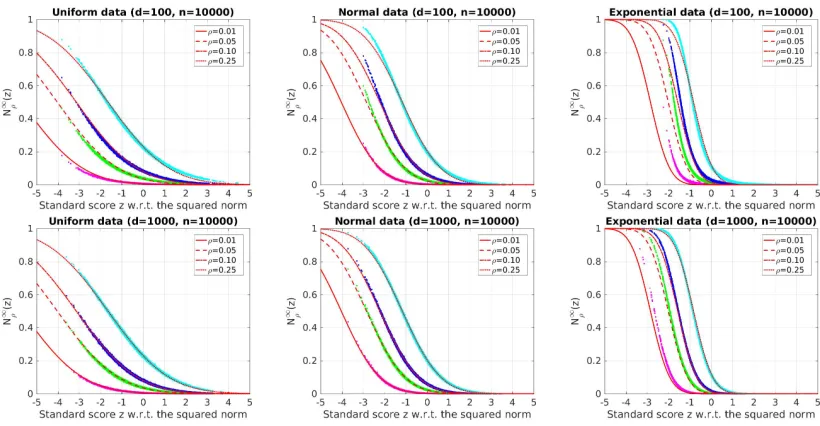
![Figure 8: [Best viewed in color.] Cumulative distribution function (left column) and prob-ability density function (right column) of the limiting distribution of the numberof k-occurrences for i.i.d](https://thumb-us.123doks.com/thumbv2/123dok_us/9789649.1964623/33.612.97.498.120.589/cumulative-distribution-function-function-limiting-distribution-numberof-occurrences.webp)
![Figure 9: [Best viewed in color.] Pairwise distance distributions for real data sets, includingthe original data (red solid line), the shuffled data (blue dashed line), and theequivalent independent data (magenta dotted line)](https://thumb-us.123doks.com/thumbv2/123dok_us/9789649.1964623/37.612.98.507.89.300/pairwise-distance-distributions-includingthe-original-shued-theequivalent-independent.webp)