Technical trading rule profitability and foreign exchange
intervention
* Blake LeBaron
Graduate School of International Economics and Finance, Brandeis University, 415 South St.,
Mailstop021, Waltham, MA 02453-2728, USA
Received 3 April 1995; received in revised form 11 March 1998; accepted 25 May 1998
Abstract
There is reliable evidence that simple rules used by traders have some predictive value over the future movement of foreign exchange prices. This paper will review some of this evidence and discuss the economic magnitude of this predictability. The profitability of these trading rules will then be analyzed in connection with central bank activity using intervention data from the Federal Reserve. The objective is to find out to what extent foreign exchange predictability can be confined to periods of central bank activity in the foreign exchange market. The results indicate that after removing periods in which the Federal Reserve is active, exchange rate predictability is dramatically reduced. 1999 Elsevier Science B.V. All rights reserved.
Keywords: Federal Reserve; Trading strategy; Bootstrap
JEL classification: F31; F33; G14; G15
1. Introduction
One of the biggest controversies between academic and applied finance is the usefulness of technical trading strategies. These rules, which intend to find patterns in past prices capable of giving some prediction of future price movements are sold as easy ways to make money, and scoffed at as charlatanism. Since the publication of Fama and Blume (1966) most academics have agreed that the
*Tel.: 11-781-736-2258; fax:11-888-420-3415.
E-mail address: [email protected] (B. LeBaron)
0022-1996 / 99 / $ – see front matter 1999 Elsevier Science B.V. All rights reserved. P I I : S 0 0 2 2 - 1 9 9 6 ( 9 8 ) 0 0 0 6 1 - 0
usefulness of these ad hoc forecasting techniques was probably close to zero. However, evidence in foreign exchange markets has been much more favorable
1
toward the usefulness of technical indicators. This technical rule predictability is strengthened by other foreign exchange puzzles such as the forward bias and
2
deviations from uncovered interest parity.
This paper looks at a possible explanation for some of the predictability found in foreign exchange markets. Using intervention series available from the Federal Reserve, predictability will be compared during periods with and without
3 4
intervention. The results of this paper are foreshadowed in this quotation from
Dooley and Shafer (1983).
At worst, central bank intervention would introduce noticeable trends into the evolution of exchange rates and create opportunities for alert private market participants to profit from speculating against the central bank. A related question is the profitability of intervention for central banks
5
themselves. However, the connection is probably not as strong as one might think initially. It depends critically on what positions the bank is taking as the foreign exchange price process moves through time. This will be discussed further in Section 6. A related question is whether the central bank is operating to stabilize or destabilize exchange rate movements, which is indirectly related to the profitability
6
of the central bank, or technical traders, and will not be addressed here.
The paper follows in four sections. First, the data series are summarized in Section 2. Section 3 reviews the results of previous work, and clearly demonstrates the magnitude of predictability in these series. Section 4 looks at predictability
1
The earliest tests were in Dooley and Shafer (1983), and Sweeney (1986) which present results consistent with some trading rule predictability. More recent studies have included Taylor (1992), LeBaron (1998), and Levich and Thomas (1993). The latter two employed bootstrap techniques to further emphasize the magnitude of the forecastability. Other related evidence includes that of Taylor and Allen (1992) which shows that a large fraction of traders continue to use technical analysis, and Frankel and Froot (1987) which shows that short term forecasts often extrapolate recent price moves.
2
Hodrick (1987), Engel (1996), and Lewis (1995) provide surveys of the large literature in this area. 3
A growing number of papers is beginning to examine this phenomenon. Szakmary and Mathur (1997) achieve similar results using monthly reserves as a proxy for intervention. Sapp (1997) shows that the results are strengthened when German interventions are used. Chaboud (1997) replicates the results using futures market data. Neely and Weller (1997) show that intervention activity might be interesting as a trading signal itself. Finally, Silber (1994) performs a similar test, but in a cross-sectional context. He shows that technical rules have value in markets where governments are present as major players.
4
For extensive surveys on the large literature on foreign exchange intervention see Edison (1993) and Almekinders (1995).
5
See Taylor (1982), Leahy (1994), and Sweeney (1996) for work in this area. 6
This debate, which goes back to Friedman (1953), is a delicate one and depends critically on the types of speculative trading going on, along with many other variables. The debate on this subject began with Baumol (1957), and continues through papers such as Szpiro (1994), where an intervening central bank can actually introduce chaos into a foreign exchange rate. Hart and Kreps (1986) provide a modern treatment displaying the full delicacy of the problem of stabilizing or destabilizing speculation.
when the Federal Reserve is not active in the market, and Section 5 addresses some issues related to simultaneity, followed by conclusions in Section 6.
2. Data summary
This study uses both weekly and daily foreign exchange series from NatWest Bank provided by DRI. The series represent the London close for the German mark (DM) and Japanese yen (JY) extending from January 2nd, 1979 through December 31st, 1992. The weekly series use the Wednesday close from this daily series. The interest rate series are 1 week Eurorates (London close) for each currency from the London Financial Times and NatWest Bank covering the same period. Summary statistics for the log first differences of the two daily foreign exchange series are given in Table 1. This table displays features that are fairly well known for relatively high frequency foreign exchange series. They are close to uncorrelated, not very skewed, showing large kurtosis.
The Federal Reserve intervention values were provided by the Federal Reserve Bank. These series represent the amount of intervention from the Federal Reserve
Table 1
Exchange rate summary statistics
DM JY Mean*100 0.003 0.012 Std.*100 0.723 0.654 Skew 0.132 0.453 Kurtosis 5.161 5.715 ACF(1) 0.012 0.015 ACF(2) 0.000 0.015 ACF(3) 0.028 0.034 ACF(4) 20.009 0.005 ACF(5) 0.029 0.037 Bartlett 0.017 0.017
Summary statistics for the daily foreign exchange series from January 2nd, 1979, through December 31st, 1992, representing 3544 daily observations of log first differences.
7
This study uses the ‘In Market’ series only. This series covers active trades made by the Federal Reserve with the intention of impacting foreign exchange rates. Passive trades instigated for reasons unrelated to exchange rate management are not included.
8
These intervention series are some of the best currently being made publicly available to researchers. However, it should be noted that there are still many improvements that would be desirable. The data used here are unable to discern between interventions coming from the Federal Reserve alone or those that are coordinated with other central banks. They also cannot capture interventions coming from third parties intervening in these two markets. Finally, some noise may still exist in estimating and dating the true intervention numbers since interventions occurring after the London close would be impacted into prices on the next day. All these effects would act against any useful findings coming from these series, so the fact that they work as well as they do in this paper is quite impressive.
7,8
in purchases (or sales) of dollars in relation to the DM or JY. All these
interventions are sterilized as mandated by Federal Reserve policy. This means that the overall monetary base is not affected by the intervention, but the
9
composition of assets will change. Some of these interventions are reported in the newspaper and are known to traders, but other interventions are secret and go
10
unreported.
Fig. 1 shows the DM / $ exchange rate plotted along with the amount of Federal
Reserve purchases(1) or sales(2) of dollars. A few important features are clear
from the picture. Firstly, intervention is a very sporadic policy with long periods in which the Federal Reserve remained calm. Secondly, there appears to be a lot of persistence to the direction of intervention in terms of purchases and sales, but overall intervention has been relatively balanced between the buying and selling sides. Finally, it is difficult to tell whether certain episodes of intervention moved the exchange rate in the desired direction simply by looking at the picture.
Table 2 gives a further summary of these intervention series. It shows that unconditionally the mean intervention levels are close to zero which is consistent with Fig. 1. However, the table shows that conditional on the intervention occurring, the mean absolute value of daily purchases or sales is near 100 million dollars. The most important numbers in Table 2 are the fraction of days that intervention is going on. For the DM this is 0.118, and for the JY this is 0.056, indicating that Federal Reserve intervention activity only occurs on a small fraction of days. The table also estimates Markov transition probabilities from no
intervention to intervention, P(I ±0uI 50), and intervention to intervention,
t t21
P(I ±0uI ±0). These estimates show that the non-intervention periods are
t t21
persistent. However, when intervention is going on it is about equally likely to continue or end on the next day. The last row reports the probability that intervention is going on in each currency given that there was an intervention in the other. Of the JY intervention days, 54% were also DM intervention days. Similarly, 27% of the DM intervention days were also JY interventions. Given that interventions are designed to affect the dollar this overlap is not surprising.
3. Trading rule evidence
This section repeats earlier statistical evidence on the forecasting properties of a simple technical trading rule. Many of these results are given in more detail in LeBaron (1998). Forecasts will be examined over 1 day and 1 week horizons. The rule used compares the current price to a moving average of past prices. Let P bet
the $ / DM exchange rate at time t. Define ma ast
9
See Dominguez and Frankel (1993) for further discussion of sterilized intervention. 10
Fig. 1. DMS / $ exchange rate and Federal Reserve purchases (1) and sales (2) of dollars for DM. M21 1 ] mat5M
O
Pt2i, (1) i50Table 2
Intervention summary statistics
DM JY Mean (I )t 22.1 21.79 Mean (uIuuI±0) 112 115 t t P(I±0) 0.118 0.056 t P(I±0uI 50) 0.065 0.029 t t21 P(I±0uI ±0) 0.584 0.532 t t21
P(I±0) given intervention against other 0.541 0.271
t
I equals the intervention at time t in millions of dollars purchased (t 1), or sold (2) in support of the dollar by the Federal Reserve. The final row displays the probability of an intervention in one currency given that there was intervention in the other market.
11
weekly M530. Define a buy or sell signal s ast
1 if Pt$mat
st5
H
21 if P,ma . (2)t t
This is an extremely trivial type of trading rule, but the strategy here is to look at the simplest versions of trading rules following common practices. This helps to reduce the impact of data snooping biases brought on by searching the entire space of trading rules for the best performers.
The application of this rule will be simplified to make some of the analysis
*
clearer. Let pt5log(P ), and r , rt t t be the domestic and foreign rates of interest, respectively. Dynamic returns from the strategy will be defined as
*
xt5s ( pt t112pt2(log(11r )t 2log(11r ))) .t (3) The value on the right side is simply the log difference on the exchange rate corrected for the interest differential. This return is then multiplied by 11 or 21 depending on the buy or sell signal. This corresponds roughly to a zero cost
12
strategy of borrowing in one currency to go long in the other. For completeness
the strategy will also be implemented without the interest rate differential,
xt5s ( pt t112p ).t (4)
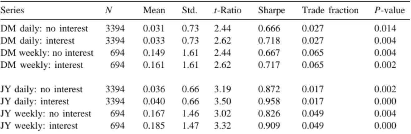
Table 3 examines these dynamic trading returns for both daily and weekly exchange rates. The t-statistics in the table test whether the mean returns are zero. It is clear from the table that the means from the dynamic strategies are statistically different from zero at any reasonable significance level. It also appears
11
Trading rule profitability is not overly sensitive to the actual length of the moving average. See LeBaron (1998) for some evidence on this. Also, these moving average lengths are very commonly used by traders.
12
The interest rates used are 1 week Eurorates. This covers the correct return span for the weekly returns. For the daily returns it is only an approximation.
Table 3 Trading rule tests
Series N Mean Std. t-Ratio Sharpe Trade fraction P-value
DM daily: no interest 3394 0.031 0.73 2.44 0.666 0.027 0.014 DM daily: interest 3394 0.033 0.73 2.62 0.718 0.027 0.004 DM weekly: no interest 694 0.149 1.61 2.44 0.667 0.065 0.004 DM weekly: interest 694 0.161 1.61 2.62 0.717 0.065 0.002 JY daily: no interest 3394 0.036 0.66 3.19 0.872 0.017 0.002 JY daily: interest 3394 0.040 0.66 3.50 0.958 0.017 0.000 JY weekly: no interest 694 0.167 1.46 3.02 0.826 0.049 0.004 JY weekly: interest 694 0.185 1.47 3.32 0.909 0.049 0.000 Tests for significance of one period trading rule returns. N is the number of observations in the sample, and mean is their mean value. t-Ratio is a t-test for the mean one period return. Sharpe is the estimated 1-year Sharpe ratio. Trade fraction is the fraction of days on which a trade takes place. P-value is the fraction of 500 simulated random walks generating a return as large as that in the actual data.
that adjusting for the interest differentials and changing from daily to weekly returns does not affect the results greatly. These t-tests may not be the proper way to test for significance because of the deviations from normality in the foreign exchange returns, so a second experiment is performed. A sample of bootstrapped random walk price series is generated using the log price differences of the original series. These differences are scrambled with replacement and a new price
13
series is built. Then the returns from the dynamic strategies, implemented on
these simulated random walk series, are compared to the original. The column labeled P-value presents the fraction of simulations generating a dynamic return larger than the original. The column agrees with the t-tests in indicating the significance of these means. The column labeled Sharpe estimates the Sharpe ratio over a 1-year horizon. This is approximated as
E(r)
]
ŒN]],
sr
wheresris the standard deviation over the short horizon. N is the number of short periods in a 1-year period. This approximation would be correct if the dynamic returns were independent over time. The values in Table 3 show that, ignoring transactions costs, Sharpe ratios in the range of 0.6–0.9 are attained. This compares with Sharpe ratios of around 0.3 or 0.4 for buy and hold strategies on
13
In the cases where interest rates are ignored this is a simple reconstruction of a random walk from the scrambled returns. In the interest rate cases, the returns less the interest rate differentials are scrambled, and rebuilt into a price series, adding the actual differentials back as the drift.
14
aggregate US stock portfolios. Finally, the column labeled ‘Trade fraction’ shows the fraction of days on which an actual trade took place, or in other words the fraction of times the strategy had to switch currencies. The low numbers here foreshadow the relatively small impact from transactions costs that will be shown in Table 4.
To better assess the economic significance of this predictability, Table 4 presents some simulation estimates of risk / return tradeoffs. One-year periods are chosen at random from the entire sample and the returns over that period are summed. After 500 of these 1-year subperiods have been chosen the mean and standard deviation are estimated and used to estimate Sharpe ratios. Different levels of transaction costs are simulated by subtracting the costs every time a trade is made (change in sign in s ). The table is in general agreement with the previoust
one for the zero cost Sharpe ratios. It also tells us that implementing the rules with a 0.1% transaction cost does not greatly reduce the Sharpe ratios which are still in
15
the range of 0.6–0.9. The table does show an eventual drop off in the Sharpe
ratio as the costs are increased. It is also clear that for the DM there are some
1-year periods in which the rule performs badly with returns less than 220%.
Another cost that will impact dynamic trading strategies of this kind is the spread between borrowing and lending rates in the offshore money markets. The numbers reported here use the offer (borrowing) interest rates for both long and short transactions. The return on loaned funds should be adjusted downward in each period according to the bid-offer spread. For the three money markets involved, the yen, dollar, and mark, this spread averages about 0.15% at an annual rate. Looking at the mean return magnitudes in Table 4 in the column labeled,
Table 4
One-year return experiments
Series Zero cost returns Sharpe ratios for varying costs
Mean Std. Max Min 0% 0.1% 0.2% 0.5%
DM daily 7.00 10.16 33.05 222.46 0.689 0.626 0.443 0.155 DM weekly 7.91 12.34 36.89 227.15 0.641 0.599 0.532 0.327 JY daily 9.73 9.41 42.97 26.35 1.033 0.981 0.864 0.670 JY weekly 10.02 10.61 44.03 29.22 0.945 0.903 0.819 0.694 Maximum, minimum, and simulated Sharpe ratios for varying transactions costs. All values are for 1-year horizon interest rate adjusted returns.
14
See Hodrick (1987), or LeBaron (1998) for some further references and examples of Sharpe ratios on aggregate portfolios. Also, see Sharpe (1994) for a summary of related work. For connections between Sharpe ratios to variance bounds tests and more information on conditional Sharpe ratios for other portfolios, see Bekaert and Hodrick (1992).
15
This transaction cost is considered a reasonable upper bound for what large traders face in foreign exchange markets in many other trading experiments such as Bilson and Hsieh (1987).
‘Mean’, it is clear that an adjustment of this magnitude would have little impact on
16
any of the numbers in the table.
In summary, this section has demonstrated significant forecastability from a simple moving average trading rule for two foreign exchange series. The results are unquestionably large statistically. Since they generate large Sharpe ratios, and their infrequent trading minimizes the impact of transaction costs, these returns appear to be economically significant as well. Another curious feature that comes out of the first two tables is that it appears that considering interest rates does not make much of a difference for these results. It is a little disturbing that interest rates have such a small impact on the results, but it is consistent with deviations from uncovered parity which suggest that in the short run exchange rate movements do not correspond closely to interest rate differentials. Another interesting fact that appears is that changing from daily to weekly frequency also does not make much of a difference. This is somewhat curious since one would expect that giving the rule the chance to trade at the daily frequency would allow it greater opportunities.
4. Removing intervention periods
This section looks at one possible explanation for the previously demonstrated puzzle in foreign exchange series, central bank intervention. Some of the previous tests are repeated with the foreign exchange intervention periods removed.
Direct evidence on the impact of intervention is presented in Table 5 where the experiments from Table 3 are repeated with intervention days removed. Returns to
the dynamic trading strategy from t to t11 are examined conditional on the
intervention series being zero on t11. For weekly series an intervention period is defined as a week in which intervention occurred on at least 1 day. The results suggest a dramatic change when intervention periods are removed. For the DM series all of the t-statistics are not significantly different from zero, and the Sharpe ratios are close to 0.1. For the JY the results are not as dramatic, but mean returns have gone into the range of only being marginally significant for two of the series, and showing simulated P-values of 0.146 and 0.198 for the other two.
These results are strong in suggesting that something different is going on when the Federal Reserve is active in terms of foreign exchange predictability. Before concluding that this is the overall cause of what is going on, some further experiments will be performed. It is possible that the clustering of intervention
16
This estimate depends on the independence of the spread and the trading rule signal. In other words the adjustment might be larger if the buy currency had larger interest rate spreads most of the time. However, it seems unlikely any dependence would have a big impact here since the magnitudes of the spreads are generally very small; 99% of the spreads fall below 1% annual for all three currencies. The maximum spreads for the dollar, mark, and yen, respectively, are 3%, 2%, and 2%.
Table 5
Trading rule statistical tests: no intervention
Series N Mean Std. t-Ratio Sharpe Trade fraction P-value
DM daily: no interest 2992 0.006 0.706 0.502 0.146 0.027 0.178 DM daily: interest 2992 0.008 0.707 0.635 0.185 0.027 0.202 DM weekly: no interest 519 0.027 1.604 0.385 0.122 0.073 0.344 DM weekly: interest 519 0.035 1.606 0.498 0.158 0.073 0.218 JY daily: no interest 3205 0.0135 0.626 1.220 0.344 0.017 0.146 JY daily: interest 3205 0.017 0.627 1.543 0.434 0.017 0.080 JY weekly: no interest 606 0.062 1.368 1.112 0.326 0.054 0.198 JY weekly: interest 606 0.080 1.374 1.441 0.422 0.054 0.106 Tests for significance of one period trading rule returns with intervention periods removed, It1150. N is the number of observations in the sample, and mean is their mean value. t-Ratio is a t-test for the mean one period return. Sharpe is the estimated 1-year Sharpe ratio. Trade fraction is the fraction of days on which a trade takes place. P-value is the fraction of 500 simulated random walks generating a return as large as that in the actual data.
periods may not have been accounted for by the tests run so far. Using the probabilities from Table 2, a two state Markov process for interventions is
ˆ
generated. Simulated interventions are given by I , where this series takes onlyt
values of 0 or 1, for no intervention, or intervention, respectively. These simulated series are aligned with the actual returns, and the returns without intervention
ˆ
(It1150) are estimated. Table 6 shows the results removing this artificial
intervention process. The table repeats the mean returns from the original series with and without intervention as well as the mean from 500 simulations removing the simulated intervention series. In each case only the results including interest adjustment are reported. The mean and variance from these simulations show the distribution to be much closer to that from the original series than the no intervention series. Finally, the P-value records the fraction of simulations giving a return lower than the no intervention series. For all the series this is close to zero. These results suggest that there really is something different about the intervention
Table 6
Markov comparisons
Mean Mean no int Markov mean Markov variance P-value
DM daily 0.033 0.008 0.033 0.005 0.002
DM weekly 0.161 0.035 0.156 0.038 0.004
JY daily 0.039 0.017 0.040 0.003 0.002
JY weekly 0.185 0.080 0.186 0.022 0.002
Trading returns are estimated removing a simulated intervention series. Mean and Mean no int. repeat the earlier mean returns with and without intervention periods. Markov mean is the mean from the 500 iterations of the simulated series. The P-value shows the fraction of the simulation runs giving a mean return as large as the no intervention series from the original intervention data.
series, and it is unlikely that randomly removing points would give the results in Table 5.
The next table presents some explorations into the dynamics of intervention periods and rule predictability to get some idea of what the mechanism is that is driving these results. Table 7 shows estimates of the probability of equal signs for
s , It t11, and the raw returns from t to t11. All of these results are conditioned on
It11 being non-zero. The first column shows the estimated probability of equal
signs between the trading rule signal and next period’s intervention. The values for both the DM and JY are very large, close to 0.8, which is significantly different from a random sign pattern of 0.5. This connection shows that when the rule indicates to buy DM, the Federal Reserve is likely to be trying to support the dollar next period. This is consistent with the rule working because of a ‘leaning against the wind’ policy with the central bank and technical traders moving in opposite directions. The second column shows the connection between the signal sign and the actual return sign next period. This connection is probably clear from some of the early tables. However, it is interesting that the sign connection is so dramatically large. This confirms that the earlier results are not driven by a few very large returns. Finally, the table presents the sign connection between the intervention and the return of each currency. This shows that on the day of the intervention it is likely that the exchange rate moves against the intervention which
17
is also consistent with a ‘leaning against the wind’ story.
One final question that might be interesting to ask is whether there is a different impact depending on whether the interventions are known or unknown. This issue is addressed in terms of the effectiveness of foreign exchange intervention in Dominguez and Frankel (1993). The previous tests are recreated in shortened form in Table 8 using their news reports of intervention. The reduction in predictability seen previously is repeated using this reported intervention series. These results should be taken with a little caution since this is a shorter series, but it appears not
Table 7 Sign comparisons
Series N Signal–Intervention Signal–Return Intervention–Return
DM daily 402 0.806 0.642 0.694
(0.025) (0.025) (0.025)
JY daily 189 0.868 0.661 0.630
(0.036) (0.036) (0.036)
Sign comparisons between the buy(1) / sell(2) signal, s , and intervention, It t11, the buy(1) / sell(2) signal returns, (t,t11), and intervention and returns. All are conditional on I ±0. Numbers in
t11 parentheses are standard errors under sign independence.
17
For this last experiment the simultaneity bias may be severe in that the Federal Reserve intervention may be induced by a desire to reverse the direction of the exchange rate. This finding has been documented by many other authors including Dominguez and Frankel (1993).
Table 8
Trading rule statistical tests: news of intervention removed
Series (daily) N Mean Std. t-Ratio Sharpe
DM: no days removed 1793 0.041 0.727 2.385 0.898
DM: US CB news removed 1592 0.025 0.692 1.415 0.565 DM: German CB news removed 1617 0.020 0.695 1.174 0.465 DM: both CB news removed 1496 0.014 0.687 0.786 0.324
JY: no days removed 1793 0.045 0.656 2.892 1.089
JY: US CB news removed 1592 0.018 0.597 1.212 0.484 JY: Japan CB news removed 1662 0.028 0.634 1.805 0.706 JY: both CB news removed 1530 0.014 0.594 0.917 0.374 Central bank intervention removed based on reports in the New York Times, the Wall Street Journal, and the Financial Times. The news series are from Dominguez and Frankel (1993). The time period is from 4 / 27 / 83–12 / 31 / 90, for a total of 1943 daily observations. All of the returns include interest rate adjustments.
to be critical whether the actual or reported interventions are removed. Another interesting extension allowed by the news series is that interventions from both the German and Japanese central banks can now be removed from the series as well. Removal of both central bank interventions reduced the Sharpe ratios to their lowest levels for both series. The changes to the JY were especially dramatic with the t-ratio dropping to 0.917 when both interventions were removed.
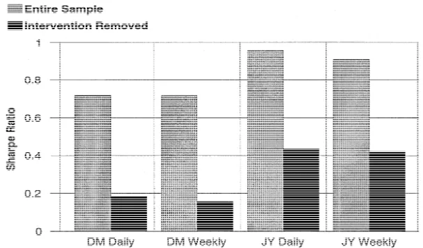
The results in this section can be summarized graphically in Fig. 2. This picture clearly shows the dramatic reduction in Sharpe ratios for the trading rules for each of the series. While conclusions about causality cannot be made, these results are
Fig. 2. The impact of removing foreign exchange intervention periods on the Sharpe ratio for the dynamic trading strategy.
very suggestive that Federal Reserve activity has something to do with the observed predictability. The next section explores the possibility that there is a common driving process causing the correlation between technical predictability and intervention.
5. Simultaneity and intervention
If a common process drives both predictability and intervention then it is clear that interventions can no longer be held responsible for setting up the conditions that make technical trading profitable. Unfortunately, all the tests here are indirect,
18
and a direct test of causality is probably unattainable with data of this frequency. Three indirect experiments are provided to test the common shock hypothesis.
The first test attempts to see if the currency the intervention is directed at is important, or if there are general time periods when intervention and profitability are likely in both the DM and JY markets. If the causality runs from technical trading predictability to later interventions, then it would seem likely that the boundaries are relatively fuzzy both across time, and exchange rate series. This would imply that removing either intervention series would do a good job in reducing the profitability of the trading strategy. In Table 9 the JY intervention days are removed from the DM series, and the DM intervention days are removed from the JY series. Days on which intervention occurs in both currencies are
19
removed from both. The purpose of this is to test whether there is something
important about the direct intervention numbers or whether all intervention happens to occur in periods that are dominated by trending currencies. The table repeats the earlier results of Table 5 for two daily series. The strong reduction in significance and Sharpe ratios seen before is clearly not present in these results. This brings into question any model with a common shock across both the DM and JY series causing predictability and intervention to occur simultaneously.
Table 9
Trading rule statistical tests: reversed intervention removed
Series N Mean Std. t-Ratio Sharpe Trade fraction P-value
DM daily 3205 0.022 0.721 1.756 0.494 0.027 0.012
JY daily 2992 0.026 0.626 2.296 0.669 0.017 0.012
Intervention periods are removed for the other currency. DM intervention periods are removed from the JY series, and JY intervention periods are removed from the DM series. Both series are interest rate adjusted.
18
Goodhart and Hesse (1993) provide tests at higher frequencies. 19
From Table 2 about 58% of the DM interventions days are also JY intervention days, and about 27% of the JY intervention days are DM intervention days. This overlap should make it difficult to see any change when using the other currencies intervention numbers.
Fig. 3. Change in strategy return for varying displacements. Intervention removal is varied from contemporaneous (0) to a 3-day lead (1) and lags (2). In other words,12 refers to the removal of days on which an intervention will occur 2 days in the future. The sample is restricted to days without interventions in the 3 days surrounding the intervention.
A second related test of the specific connection between the trading rule profitability and intervention activity is to check the time pattern of the reduction in trading rule profitability. Fig. 3 reports the percentage change in return to the trading strategy if days before or after interventions are removed. The intervention series is reduced to those interventions without interventions during the 3 days before or after. The positive displacements in Fig. 3 refer to removing days that lead an intervention by 1, 2, and 3 days respectively. The negative displacements remove days that follow interventions. The picture shows a clear pattern that the
20
exact intervention day is where almost all of the changes are coming from. It
would seem plausible that other common factors causing trading profitability and interventions might be relatively slow moving. If this were the case then removing nearby days should have almost as large an effect as removing the exact intervention day. This does not appear to be the case. If there is a common factor it is a very short lived phenomenon.
One possible factor that might drive both predictability and interventions is volatility. Excessively volatile periods might be ones in which central banks are
20
21
intervening heavily to try to stabilize markets. Also, high volatility periods might add extra risk to dynamic strategies implying a higher risk premium, and therefore greater predictability. This hypothesis is tested in Table 10 where volatility is
22
estimated using a GARCH(1,1) model. This model forecasts volatility as a
function of lagged squared returns,
2
ht5a 1 b0 ht211a1 tr21.
Since the intervention periods account for about 10% of the samples, all days are removed whose expected volatility lies in the upper 10% of the overall volatility distribution for each foreign exchange series. Results of the basic trading rule tests with these volatile periods removed are presented in Table 10. There is little change here from the results in Table 3 in that the trading rules are still performing well. Therefore it is unlikely that a single volatility related factor could be driving both interventions and predictability.
The perfect experiment to test for causality versus simultaneity hypothesis would be to have a time period where for some reason interventions were outlawed as a policy. There is a close proxy to this in the period from 1981–1984. During this time period, The Under Secretary for Monetary Affairs, Beryl
23
Sprinkel, announced an explicit non-interventionist policy. Observation of actual
series in Fig. 1 shows that there were a few interventions during this time, but they were sporadic and small in magnitude. Table 11, panel A, repeats the tests of Table 3 for this time period alone. The results here show little predictive ability for the trading rules during this time period with limited interventions which is supportive of the hypothesis that interventions themselves are important to the technical trading predictability. A final subsample is tested in panel B of Table 11.
Table 10
Trading rule returns: volatile periods removed
Series N Mean Std. t-Ratio Sharpe T fraction
DM daily 3394 0.033 0.73 2.62 0.718 0.027
DM daily: vol. removed 3064 0.044 0.69 3.49 1.004 0.026
JY daily 3394 0.034 0.66 3.50 0.958 0.017
JY daily: vol. removed 3064 0.038 0.63 3.34 0.963 0.017 Upper 10% of expected volatility days are removed. Conditional volatility is estimated using a GARCH(1,1). Original results are included for comparison. Both series are interest rate adjusted.
21
Dominguez (1993) presents some evidence indicating that interventions have led to reductions in volatility.
22
The ARCH / GARCH models developed in Engle (1982) and Bollerslev (1986) are surveyed in Bollerslev et al. (1990), (1995).
23
Table 11
Trading rule tests: 1981–1984, 1993–1995
Series N Mean Std. t-Ratio Sharpe T fraction
Panel A: 1981–1984 DM daily 862 0.001 0.686 0.025 0.013 0.039 JY daily 862 0.018 0.625 0.842 0.457 0.019 Panel B: 1993–1995 DM daily 780 20.010 0.685 20.420 20.240 0.030 JY daily 780 0.022 0.723 0.861 0.487 0.017
Trading rule tests during low intervention periods. During the first subperiod explicit policy stated that foreign exchange intervention would not be used. During the later subperiod, intervention has been used sparingly. There were interventions against the DM and JY, respectively, on 1.8, and 2.2% of trading days.
This refers to the recent 3-year period from 1993–1995 which is outside the previous sample. Although not as explicit as in the previous period, it appears that Federal Reserve policy on interventions has been changing over this time. In a recent article, Muehring (1997) documents that Federal Reserve intervention policy is moving in the direction of transparency in all markets. It explicitly states that the interventions in the yen market in May 1995 were clearly announced to markets. The results of panel A are repeated here, in that there is very little
24
profitability for the trading rules.
Although it would be impossible to rule out the existence of a single common factor driving these results, these three experiments make it look unlikely that it will be easy to find.
6. Conclusions
The fact that simple trading rules produce unusually large profits in foreign exchange series presents a serious challenge to the efficient market hypothesis. Further, the magnitude of these returns and their resiliency to the adjustment for transactions costs makes it difficult to imagine a representative agent rational expectations model capable of explaining these results. However, foreign exchange markets differ from most other major asset markets in that there are several major players whose objectives may differ greatly from those of maximizing economic agents. The results in this paper show that this predictability puzzle is greatly reduced, if not eliminated, when days in which the Federal Reserve was actively intervening are eliminated.
Before quickly concluding a causal relationship between intervention and
24
This was also a period when interventions were relatively infrequent. The Federal Reserve intervened in the DM market on 1.8% of days, and the JY market 2.2%.
trading rule profitability there is a serious simultaneity problem that needs to be addressed. Interventions and profits may be driven by the same common factor and therefore the apparent causal relation might be spurious. This hidden factor can never be completely eliminated as a potential cause, but this paper explored several possible ways in which it might appear. The results of these experiments make it look unlikely that a common factor will be easy to find.
The policy recommendations are not as clear cut as they might seem. If the Federal Reserve is transferring money to traders, it may be worthwhile in that it has other variables in its objective function such as overall price stability. Stopping a potential trade war may far outweigh a few losses in the foreign exchange market. It is also interesting that other studies such as Leahy (1994) find that the Federal Reserve is making money on its foreign exchange intervention operations. This fact, while an interesting contrast to the results here, is not exactly a contradiction since the magnitudes of interventions or total bank positions have not been analyzed here.
Understanding the causes and structure of this apparent predictability in foreign exchange markets is important both from the standpoint of understanding the forces that drive exchange rate movements, but also for implementing appropriate policies. These results are still far from implicating the Federal Reserve in this puzzle, but they may make those whose biases are toward efficient markets a little more comfortable, while revealing a troubling lack of robustness for technical signal predictability.
Acknowledgements
The author is grateful to the Alfred P. Sloan Foundation and the University of Wisconsin Graduate School for support. The author thanks Kathryn Dominguez, Robert Hodrick, Maria Muniagurria, seminar participants at the Federal Reserve Board of Governors, The Federal Reserve Bank of New York, Brandeis, Iowa St. University, and the NBER for helpful comments. The author is also grateful to Kathryn Dominguez for kindly providing the intervention news series.
References
Almekinders, G.J., 1995. Foreign Exchange Intervention: Theory and Evidence. E. Elgar, Brookfield, VT.
Baumol, W., 1957. Speculation, profitability, and stability. Review of Economics and Statistics 39, 263–271.
Bekaert, G., Hodrick, R.J., 1992. Characterizing predictable components in excess returns on equity and foreign exchange markets. Journal of Finance 47, 467–511.
Bilson, J.F., Hsieh, D., 1987. The profitability of currency speculation. International Journal of Forecasting 3, 115–130.
Bollerslev, T., 1986. Generalized autoregressive conditional heteroskedasticity. Journal of Econo-metrics 21, 307–328.
Bollerslev, T., Chou, R.Y., Jayaraman, N., Kroner, K.F., 1990. ARCH modeling in finance: a review of the theory and empirical evidence. Journal of Econometrics 52 (1), 5–60.
Bollerslev, T., Engle, R.F., Nelson, D.B., 1995. ARCH models, in: Handbook of Econometrics, vol. 4. North-Holland, New York.
Chaboud, A., 1997. Technical trading profitability in foreign exchange futures markets and federal reserve intervention. Technical report, University of Wisconsin, Madison, WI.
Dominguez, K.M., 1993. Does central bank intervention increase the volatility of foreign exchange rates? Technical Report 4532, National Bureau of Economic Research, Cambridge, MA. Dominguez, K.M., Frankel, J.A., 1993. Does Foreign Exchange Intervention Work? Institute for
International Economics, Washington, DC.
Dooley, M.P., Shafer, J., 1983. Analysis of short-run exchange rate behavior: March 1973 to November 1981. In: Bigman, D., Taya, T. (Eds.), Exchange Rate and Trade Instability: Causes, Consequences, and Remedies. Ballinger, Cambridge, MA.
Edison, H.J., 1993. The Effectiveness of Central-bank Intervention: A Survey of the Literature After 1982. Number 18 in Special Papers in International Economics, Department of Economics, Princeton University, Princeton, NJ.
Engel, C., 1996. The forward discount anomaly and the risk premium: a survey of recent evidence. Journal of Empirical Finance 3, 123–192.
Engle, R.F., 1982. Autoregressive conditional heteroskedasticity with estimates of the variance of United Kingdom inflation. Econometrica 50, 987–1007.
Fama, E.F., Blume, M., 1966. Filter rules and stock market trading profits. Journal of Business 39, 226–241.
Frankel, J.A., Froot, K.A., 1987. Using survey data to test standard propositions regarding exchange rate expectations. American Economic Review 77 (1), 133–153.
Friedman, M., 1953. The case for flexible exchange rates. In: Essays in Positive Economics. University of Chicago Press, Chicago, IL.
Goodhart, C.A.E., Hesse, T., 1993. Central bank forex intervention assessed in continuous time. Journal of International Money and Finance 12, 368–389.
Hart, O.D., Kreps, D.M., 1986. Price destabilizing speculation. Journal of Political Economy 94, 927–952.
Hodrick, R.J., 1987. The Empirical Evidence on the Efficiency of Forward and Futures Foreign Exchange Markets. Harwood Academic Publishers, New York.
Klein, M.W., 1993. The accuracy of reports of foreign exchange intervention. Journal of International Money and Finance 12 (6), 644–653.
Leahy, M., 1994. The profitability of US intervention. Journal of International Money and Finance 14 (6), 823–844.
LeBaron, B., 1998. Technical trading rules and regime shifts in foreign exchange. In: Acar, F., Satchell, S. (Eds.), Advanced Trading Rules. Butterworth-Heinemann, pp. 5–40.
Levich, R.M., Thomas, L.R., 1993. The significance of technical trading-rule profits in the foreign exchange market: a bootstrap approach. Journal of International Money and Finance 12, 451–474. Lewis, K., 1995. Puzzles in international financial markets. In: Grossman, G.M., Rogoff, K. (Eds.),
Handbook of International Economics, vol. 3. North Holland, Amsterdam, pp. 1913–1971. Muehring, K., 1997. The Feds repo man. Institutional Investor, April, pp. 45–48.
Neely, C., Weller, P., 1997. Technical analysis and central bank intervention. Technical report, Federal Reserve Bank of St. Louis, St. Louis, MO.
Sapp, S., 1997. Foreign exchange markets and central bank intervention. Technical report, J.L. Kellogg Graduate School of Management, Northwestern University, Evanston, IL.
Sharpe, W.F., 1994. The Sharpe ratio. Journal of Portfolio Management 21 (1), 49–58.
Silber, W.L., 1994. Technical trading: when it works and when it doesn’t. The Journal of Derivatives 1 (3), 39–44.
Sweeney, R., 1996. Do central banks lose on foreign-exchange intervention? A review article. Technical report, Georgetown University, Washington, DC.
Sweeney, R.J., 1986. Beating the foreign exchange market. Journal of Finance 41, 163–182. Szakmary, A.C., Mathur, I., 1997. Central bank intervention and trading rule profits in foreign
exchange markets. Journal of International Money and Finance 16, 513–535.
Szpiro, G.G., 1994. Exchange rate speculation and chaos inducing intervention. Journal of Economic Behavior and Organization 24, 363–368.
Taylor, D., 1982. Official intervention in the foreign exchange market, or, bet against the central bank. Journal of Political Economy 90 (2), 356–368.
Taylor, M., Allen, H., 1992. The use of technical analysis in the foreign exchange market. Journal of International Money and Finance 11 (3), 304–314.
Taylor, S.J., 1992. Rewards available to currency futures speculators: compensation for risk or evidence of inefficient pricing?. Economic Record 68, 105–116.