http://www.sciencepublishinggroup.com/j/ajwse doi: 10.11648/j.ajwse.20180404.15
ISSN: 2575-1867 (Print); ISSN: 2575-1875 (Online)
Estimation of Potential Evapotranspiration by Different
Methods in Handan Eastern Plain, China
Yinqin Zhang
School of Water Conservancy and Hydroelectric Power, Hebei University of Engineering, Handan, China
Email address:
To cite this article:
Yinqin Zhang. Estimation of Potential Evapotranspiration by Different Methods in Handan Eastern Plain, China. American Journal of Water Science and Engineering. Vol. 4, No. 4, 2018, pp. 117-123. doi: 10.11648/j.ajwse.20180404.15
Received: November 28, 2018; Accepted: December 25, 2018; Published: January 18, 2019
Abstract:
Potential evapotranspiration estimation is the foundation of water resources assessment. Based on the daily meteorological data during 2000-2005 of Linzhang Meteorological Station in Handan Eastern Plain, temperature-based Hargreaves method, radiation-based Priestley-Taylor method, and FAO Penman-Monteith method with comprehensive consideration of aerodynamics were used to estimate potential evapotranspiration. Correlations between monthly potential evapotranspiration and water surface evaporation were conducted. The results indicated that potential evapotranspiration calculated by Hargreaves method was the largest, while the potential evapotranspiration calculated by Priestley-Taylor method was the smallest. The seasonal potential evapotranspiration values for the three methods were summer > spring > autumn > winter. The correlation between potential evapotranspiration calculated by the FAO Penman-Monteith method and water surface evaporation during the same period was best (r=0.991). In contrast, Penman-Monteith method is more suitable for estimating the potential evapotranspiration in Handan Eastern Plain.Keywords:
Potential Evapotranspiration, Hargreaves Method, Priestley-Taylor Method, Penman-Monteith Method, Water Surface Evaporation, Handan Eastern Plain1. Introduction
Potential evapotranspiration (ETP) is defined as the amount of water that would be evaporated and transpired by a specific crop or ecosystem if there were sufficient water available [1].
ETP is the theoretical upper limit of actual evapotranspiration.
ETP can be estimated indirectly from climatological parameters such as minimum and maximum air temperatures, sunshine hours, actual vapor pressure, relative humidity, wind speed, solar radiation, extraterrestrial solar radiation, net radiation, etc. [2, 3]. Several different methods were used to calculate ETP in hydrologic models [4-8]. Generally, methods for estimating ETP can be roughly divided into three categories, that is, temperature based method, radiation based method and synthetic method. Six temperature based methods (Blaney-Criddle, Kharrufa, Hargreaves and Samani, Oudin, Thornthwaite, Hamon) were selected to estimate ETP in Shannon River catchment. The study found that the Hamon method performed best in comparison with the Met Éireann data [9]. In a Two-Source Model, latent heat flux was computed on the basis of Priestley-Taylor method [10].
Additionally, three temperature based (Thornthwaite, Hamon, and Hargreaves-Samani) and three radiation based (Turc, Makkink, and Priestley-Taylor) methods were used to calculate ETP simultaneously in the southeastern United States. Results indicated that the Priestley-Taylor, Turc, and Hamon methods produced more precise results than the other ETP methods [3]. Penman-Monteith formula was the most widely
ETP method and normally used as a standard term to evaluate the accuracy of other ETP method [8, 11].
In this study, Hargreaves method (H method) based on temperature, Priestley-Taylor method (P-T method) based on radiation and FAO Penman-Monteith method (P-M method) taken aerodynamics into account were employed to compute
mainly concentrated during July to September, accounting for 60% of annual precipitation. Mean annual evaporation of water surface in this area (E601 evaporation pan) varies from1007mm to 1266mm [12].
2. Methods
2.1. ETp Estimation
2.1.1. Hargreaves Method
Hargreaves method is an alternative approach and proposed based on the following empirical formula using mean maximum and minimum temperature as well as extraterrestrial radiation data [13-15].
0.0135 17.8
2
max min
H s
T T
ET = R + +
(1)
2 E max min
s RS a
T T R =K R +
(2)
where ETH is potential evapotranspiration calculated by Hargreaves method, mm/d; Tmax and Tmin are maximum and minimum temperature, respectively, °C; Rsis solar radiation,
mm/d; KRSis an empirical coefficient; Rais the extraterrestrial radiation, mm/d; E is a parameter of the equation (2).
Substitute equation (2) into equation (1), ETH can be expressed as:
(
)
2
E max min
H a max min
T T ET =CR T −T + +T
(3)
where C, E and T are parameters of the Hargreaves equation; Values of 0.0023 (KRS=0.16, C=0.0135KRS), 0.5 and 17.8 are recommended, respectively.
Then Hargreaves equation was represented as:
0.0023 17.8
2
max min
H a max min
T T
ET = R + + T −T
(4)
where Ra was calculated by station latitude and expressed as:
( )
(
) (
)
24 60
sin sin cos cos sin
a sc r s s
R G d ω ϕ δ ϕ δ ω
π
= + (5)
where Gsc is solar constant, Gsc=0.082MJ⋅m-2 ⋅min-1; dr is the earth-sun distance; ωsis solar altitude.
dr was expressed by:
2 1 0.033cos
365
r
d = + π J
(6)
where J=1, 2,…, 365 or 366.
( )
s arccos tan tan( )
ω = − ϕ δ (7)
2
=0.409sin 1.39
365J π
δ −
(8)
2.1.2. Priestley-Taylor Method
Priestley-Taylor method is a kind of radiation based method for estimating potential evapotranspiration [16-17]. The Priestley-Taylor equation is expressed as:
1.28 ( )
p n
ET R G
γ ∆
= × × −
∆ + (9)
where Rn is net radiation, MJ⋅ m -2⋅
d-1; G is soil heat flux, MJ⋅ m-2⋅ d-1; G can be ignored for day period; Δ is slope of
saturation vapor pressure curve at air temperature, kPa⋅°C-1;γ
is psychrometric constant, kPa⋅°C-1.
For Δ, γ and P, the respective computational formula was
presented by:
(
)
217.27
4098 0.6108 exp( )
237.3 = 237.3 T T T × + ∆
+ (10)
3 0.665 10 P
γ
= × − ×(11) 5.26 293 0.0065 101.3 293 z P= × −
(12)
where P is atmospheric pressure, kPa; z is elevation above sea level of meteorological station, m.
Rnwas calculated as follows:
n ns nl
R = R - R (13)
( )
ns s
R = 1 - a R (14)
s s s a
n R a b R
N
= +
(15)
(
)
4 4
, ,
= 0.34 0.14 (1.35 0.35)
2
max k min k s
nl a
so
T T R
R e
R
σ + − −
(16)
5
(0.75 2 10 )
so a
R = + × − z R (17)
0
e ( )
100 mean
a mean
RH e T
= (18)
2
max min mean
T +T
T = (19)
0 17.27
( )=0.6108 ( ) 237.3 mean
T
e T exp
T+ (20)
where Rns is net shortwave radiation, MJ⋅ m-2⋅ d-1; Rnlis net longwave radiation, MJ⋅ m-2⋅ d-1; Rs is solar radiation or shortwave radiation, MJ⋅ m-2⋅ d-1; n is actual duration of sunshine, hr; Here, contemporaneous data of adjacent Anyang station (station index number is 53898) are given to n; N is maximum possible duration of sunshine or daylight hours, hr; Default values of as=0.25 and bs=0.5 are used;σ=4.903 10× -9;
humidity; Tmean is the mean air temperature;
(
)
0mean
e T
issaturation vapor pressure at the air temperature at the temperature of Tmean.
2.1.3. FAO Penman-Monteith Method
Penman-Monteith equation was proposed by the Food and Agriculture Organization (FAO) for estimating ETp only based on meteorological data [18-19]. The calculation formula of FAO Penman-Monteith method is expressed as:
900
0.408 ( ) ( )
273 (1 0.34 )
n 2 s a
P -M
2
R G u e e
T ET u γ γ ∆ − + − + =
∆ + + (21)
( ) ( )
+ = 2 0 0 max min se T e T
e (22)
where T is the mean daily temperature, °C; u2 is wind speed at 2m above ground surface, m/s;es is the saturation vapor
pressure, kPa; es-ea is the vapor pressure deficit, kPa.
Based on daily meteorological data of Linzhang Meteorological Station in Handan Eastern Plain, ETp at different time scales (monthly, seasonal and annual) were estimated using three different methods as mentioned above.
2.2. Mann-Kedall Non-Parametric Test Method
Mann-Kedall (M-K) method is a non-parametric test method [20-21]. The specific calculation steps for M-K method are described as follows:
Firstly, mathematical formula for a statistic was expressed as:
(
)
-1 1 1 -n n j i i j nS sgn x x
= = +
=
∑ ∑
(23)(
-)
1 0 1j i
j i j i
j i
x x
sgn x x x x
x x > = = − < (24)
where S is a statistic; sgn is sign function; xi and xj is target variables of the ithand jth,respectively; n is sample number.
When n is greater than 8, S will approximately obey the normal distribution with the mean of zero and variance of
Var(S).
( )
0E S = (25)
( )
n n(
1 (218)
n 5)Var S = − + (26)
where E(S) is the mean of S; Var(S) is the variance of S. Then the test statistic of M-K method was represented as:
1 0 (S) 0 0 1 0 (S) S S Var Z S S S Var − > = = −
<
(27)
where Z is the test statistic; Z > 0 shows that the corresponding time series has an increasing trend; On the contrary, Z < 0 shows that the time series has an decreasing trend.
2.3. Pearson’s Correlation Coefficient
Pearson’s correlation coefficient is a measuring index of the correlation degree between two variables [22]. The calculation formula of the correlation coefficient is expressed as:
(
)
( , ),
[ ] [ ]
Cov X Y r X Y
Var x Var Y
= (28)
where r is Pearson’s correlation coefficient; r ranges from -1 to 1. The closer r gets to 1, the higher the correlation is.
Cov(X,Y) is the covariance between X and Y; Var[X] and
Var[Y] refer to the variance of X and Y, respectively.
3. Results and Discussions
3.1. Variations of Potential Evapotranspiration at Different Time Scales
3.1.1. Monthly Potential Evapotranspiration
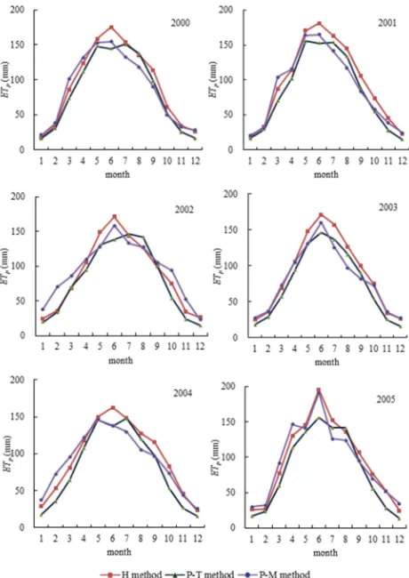
Based on the equations mentioned in sections 2.1-2.3, monthly ETH, ETP-T and ETP-M were calculated (Figure 1). H method requires minimum, maximum and mean temperature as well as extraterrestrial radiation. Estimated mean monthly
ETH ranged from 23.5mm to 176.2mm. P-T method uses net radiation, slope of saturation vapor pressure curve at air temperature, atmospheric pressure, etc. to estimate ETP-T. And the corresponding mean monthly ETP-T values were between 15.1mm and 146.2mm. Besides radiation data, P-M method also includes mean daily temperature, wind speed, vapor pressure deficit. The calculated mean monthly ETP-M varied from 27.2mm to 161.3mm. Hence, the results obtained by three methods were different, which may be attributed by the different types of data employed in H method, P-T method and P-M method. Take P-M method as the standard, previous study found that the radiation-based methods performed better than temperature-related methods on the island of Crete in Southern Greece [8].
ETP-M values were greater than that of ETP-T. It may be attributed by heat and aerodynamics considered in P-M method. In addition, variation trends of potential evapotranspiration calculated by three methods (H, P-T and P-M method) were relatively consistent. The overall trend increased firstly and then decreased. H method had good agreement with P-M method. From July to September, ETP-T values were larger than that of P-M method. For other months,
ETP values were low. Taking the Loess Plateau of northern Shaanxi for example, the sensitivity of potential evapotranspiration to the variation of each meteorological factor was different. Related study demonstrated that ETp was most sensitive to relative humidity, followed by daily maximum temperature, wind speed, sunshine hours, and daily minimum temperature [23].
Figure 1. Monthly potential evapotranspiration calculated by different methods.
3.1.2. Seasonal Potential Evapotranspiration
Variations in potential evapotranspiration for different seasons were shown in Figure 2. Herein, March to May, June to August, September to November, December to February in the following year were considered to be Spring, Summer, Autumn and Winter, respectively. Potential evapotranspiration calculated by H method, P-T method and P-M method was Summer, Spring, Autumn and Winter from large to small. Specifically,
ETH varied from 438.3mm to 493.0mm in Summer, 324.1mm to 372.3mm in Spring, 208.2mm to 244.2mm in Autumn, 74.8mm to 104.6mm in Winter. ETP-T ranged from 391.4mm to 440mm in
Summer, 281.2mm to 331.9mm in Spring, 168.3mm to 178.1mm in Autumn, 53.4mm to 68.5mm in Winter. ETP-Mwas between 373.3mm and 445.5mm in Summer, 308.4mm and 386mm in Spring, 172.1mm and 255.4mm in Autumn, 76.1mm and 160.7mm in Winter. Qi et al. found that the average reference evapotranspiration calculated by P-M method was 248mm in Spring, 312mm in Summer, 134mm in Autumn, and 35mm in Winter from 1964 to 2013 in Heilongjiang Province, Northeast China [11].
In general, seasonal difference between H method and P-T method varied little in this study. For example, difference of ETH in Summer and Spring was approximately equal to the difference of ETH between Spring and Autumn. By contrast, ETP-M in different seasons was rather changeable. In addition, evapotranspiration sensitivity factor may be different seasonally. Previous study pointed that relative humidity was the most sensitive factor in Spring, Summer and Autumn while Tmax was most sensitive in Winter in Heilongjiang Province [11].
Figure 2. Seasonal variations of potential evapotranspiration calculated by different methods.
3.1.3. Annual Potential Evapotranspiration
Annual potential evapotranspiration was derived from the sum of monthly potential evapotranspiration (Table 1). In general,
Annual ETH was overestimated and the maximum and minimum values occurred in 2002 and 2003, separately. While ETP-Tvalues were the lowest and the respective maximum and minimum values appeared in 2000 and 2003. In term of ETP-M, the highest value was in 2005 and the lowest value was in 2003. Standard deviation of ETP-T was the least, with the value of 30.5mm. However, standard deviation of ETP-M was the largest, with the value of 50.3mm. In addition, the variation trend of ETP-Tand
ETP-M was basically consistent. Specifically, potential evapotranspiration changes decreased from 2000 to 2003 while increased from 2003 to 2005. But the amplitude of variation in
ETP-M was greater than that of ETP-T. In a similar study, researchers reported that annual reference evapotranspiration ascended 7.40 mm per decade during 1992 to 2015 in the Jing-Jin-Ji region, North China [24].
Table 1. Annual potential evapotranspiration calculated by H, P-T, and P-M methods (mm).
year ETH ETP-T ETP-M
2000 1138.9 1002.2 1051.0
2001 1159.4 997.4 1062.8
2002 1194.8 977.5 1023.4
2003 1074.7 909.4 970.3
2004 1135.5 967.0 1086.6
2005 1148.4 980.3 1132.1
It is found that there are differences among potential evapotranspiration (monthly, seasonal, annual) calculated by H, P-T and P-M methods, although the overall trend remains consistent for each time scale. As we all known, different ETp formula were proposed in the certain physical geographic conditions. When we transfer it to another region, some parameters may need to be modified so as to improve its estimating accuracy [15, 25]. In addition, ETp is influenced by many meteorological factors such as air temperature, relative humidity, solar radiation, wind speed, groundwater depth, etc. Among others, ETp was high in shallow water level areas and low in deep water level areas [26]. Previous studies carried out sensitivity analysis of meteorological parameters to ETp [27-29]. It is an ongoing work so the sensitivity analysis of
ETp to every meteorological factor was not further conducted in this study. When we ignored drawbacks mentioned above, the applicability of original equations of estimating potential evapotranspiration in this study area can be acceptable.
3.2. Correlation Between Potential Evapotranspiration and Water Surface Evaporation
3.2.1. Trend Test of Water Surface Evaporation
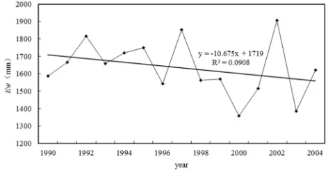
According to the observed water surface evaporation (Ew)
in Linzhang Meteorological Station, annual Ew varied from 1907.1mm to 1356.7mm during 1990-2004, with the mean annual of 1637.0mm (Figure 3). By adding a linear trend line, it is found that annual Ew had a decreasing trend. Then M-K method was employed to test its reducing significance, |Z|<
Zα/2 showed that annual Ew time series did not pass significance testing at the level of α=5% (Table 2). Thus, the corresponding decreasing trend of water surface evaporation was not significant.
Figure 3. Variations of annual water surface evaporation.
Table 2. Significance testing of water surface evaporation at annual scale by M-K method.
n S Var(S) Z Zα/2 Trend
15 -21 408.333 -0.99 1.96 non-significant
3.2.2. Correlation Analysis Between Potential
Evapotranspiration and Water Surface Evaporation at Monthly Scale
As shown in Table 3, monthly mean ETH, ETP-T, ETP-M and Ew varied from 23.3mm (December) to 174.1mm (June), 15.3mm (December) to 147.7mm (July), 24.6mm (December) to 156.4mm (June), and 26.7mm (December) to 238.4mm (June), respectively. Correlation analysis results indicated that monthly average potential evapotranspiration and water surface evaporation were all highly correlated. Pearson’s correlation coefficients of monthly ETH, ETP-T, ETP-M and Ew were 0.962, 0.925 and 0.991, respectively. In comparison, correlations between
ETP-M and Ew was superior to the others, indicating that P-M method was much more suitable for estimating potential evapotranspiration in Handan Eastern Plain. Partial correlation analysis also can be found in Han et al. [24]. The results showed that the increase of reference evapotranspiration was caused by increased average air temperature and wind speed as well as decreased relative humidity.
Table 3. Monthly average potential evapotranspiration and water surface evaporation (Ew) (mm).
Month 1 2 3 4 5 6 7 8 9 10 11 12
4. Conclusions
H method, P-T method and P-M method were used to estimate daily potential evapotranspiration in this study. Potential evapotranspiration in different time scales (monthly, seasonal, annual) were compared based on the above methods. Then the correlation coefficients between monthly potential evapotranspiration and water surface were calculated.
Results indicate that monthly potential evapotranspiration calculated from H method, P-T method and P-M method are the highest during June and July. For seasonal potential evapotranspiration, ETp values calculated by H, P-T and P-M methods are the highest in Summer and lowest in Winter. Annual ETP-Tis smaller than ETH and ETP-M in the same year. Standard deviation of annual ETP-T is the smallest (30.5mm) while standard deviation of annual ETP-M is the highest, with the value of 50.3mm. Pearson’s correlation coefficients between monthly ETHand Ew, ETP-T and Ew as well as ETP-M and Ew were all greater than 0.9. The largest correlation coefficient is 0.991 for ETP-M and Ew. By contrast, the correlation between monthly ETP-T and Ew is lowest (r=0.925). In conclusion, P-M method is much more suitable for estimating potential evapotranspiration in Handan Eastern Plain.
Acknowledgements
This study was supported by Hebei Province Natural Science Foundation for Youth (E2016402186), the doctoral specialized fund of Hebei University of Engineering, Doctoral program construction project of Hebei University of Engineering (15967663D).
References
[1] Evapotranspiration. Available from: https://en.wikipedia.org/ wiki/Evapotranspiration#Potential_evapotranspiration. [2] Srdjan J., Blagoje N., Zoran G., et al. 2018. Evolutionary
algorithm for reference evapotranspiration analysis. Comput. Electron. Agr., 150, 1-4.
[3] Lu J. B., Ge S., Steven G. M., et al. 2005. A comparison of six potential evapotranspiration methods for regional use in the southeastern United States. J. American Water Resour. Association, 621-633.
[4] Thompson J. R., Green A. J., Kingston D. G. 2014. Potential evapotranspiration-related uncertainty in climate change impacts on river flow: An assessment for the Mekong River basin. J. Hydrol., 510, 259-279.
[5] Osorio J., Jeong J., Bieger K., et al. 2014. Influence of potential evapotranspiration on the water balance of sugarcane fields in Maui, Hawaii. Journal of Water Resource and Protection, 6, 852-868.
[6] Weiß M., Menzel L. 2008. A global comparison of four potential evapotranspiration equations and their relevance to stream flow modelling in semi-arid environments. Adv. Geosci., 18, 15-23.
[7] Lang D. X., Zheng J. K., Shi J. Q., et al. 2017. A comparative study of potential evapotranspiration estimation by eight methods with FAO Penman-Monteith method in Southwestern China. Water, 9, 734.
[8] Xystrakis F., Matzarakis A. 2011. Evaluation of 13 empirical reference potential evapotranspiration equations on the island of Crete in Southern Greece. J. Irrig. Drain Eng., 137, 211-222.
[9] Salem S. Gharbia, Trevor Smullen, Laurence Gill, et al. 2018. Spatially distributed potential evapotranspiration modeling and climate projections. Sci. Total Environ., 633, 571-592. [10] Sun H. 2016. A Two-Source Model for Estimating Evaporative
Fraction (TMEF) Coupling Priestley-Taylor Formula and Two-Stage Trapezoid. Remote Sens., 8, 248.
[11] Qi P., Zhang G., Xu Y. J., et al. 2017. Spatiotemporal Changes of Reference Evapotranspiration in the Highest-Latitude Region of China. Water, 9, 493.
[12] Long Q. B. 2011. Study on sustainable water resource management in Handan Eastern Plain. Master's Thesis of Hebei University of Engineering.
[13] Hargreaves G. L., Hargreaves G. H., Riley J. P. 1985. Agricultural benefits for Senegal River basin. J. Irrig. Drain. Eng., ASCE,111(2),113-124.
[14] Hargreaves G. H., Allen R. G. 2003. History and evaluation of Hargreaves evapotranspiration equation. J. Irrig. Drain. Eng., 129:53-63.
[15] Haie N., Pereira R. M., Yen H. 2018. An Introduction to the Hyperspace of Hargreaves-Samani Reference Evapotranspiration. Sustain., 10, 4277.
[16] Priestley C. H. B., Taylor R.J. 1972. On the assessment of surface heat flux and evaporation using large-scale parameters. Mon. Weather Rev. 100, 81-92.
[17] Sun H. 2016. A Two-source Model for Estimating Evaporative Fraction (TMEF) coupling Priestley-Taylor formula and two-stage trapezoid. Remote Sens., 8(3), 248.
[18] Wang X. H., Guo M. H., Xu Z. M. 2006. Comparison of estimating ET0 in arid-area of Northwest China by Hargreaves equation and Penman-Monteith equation. Transactions of the CSAE, 22(10):21-25. (in Chinese with English abstract). [19] Allen R. G., Pereira L. S., Raes D. et al. 1998. Crop
evapotranspiration-guidelines for computing crop water requirements. FAO Irrigation and drainage paper 56. Rome, Italy: Food and Agriculture Organization of the United Nations.
[20] Mann, H. B. 1945. Nonparametric tests against trend. Econometrica 33:245-259.
[21] Kendall, M. 1975. Multivariate analysis. Charles Griffin. [22] Gao S., Wang H. W., Sang X. L., et al. 2016. Analyzing the
correlation of time series of rainfall-runoff in Yuanjiang-Red River Basin. Systems Engineering, 34 (3): 153-158. (in Chinese with English abstract)
[24] Han J. Y., Wang J. H., Zhao Y., et al. 2018. Spatio-temporal variation of potential evapotranspiration and climatic drivers in the Jing-Jin-Ji region, North China. Agr. Forest Meteorol., 256-257, 75-83.
[25] Ding R., Kang S., Li F., et al. 2013. Evapotranspiration measurement and estimation using modified Priestley-Taylor model in an irrigated maize field with mulching. Agric. For. Meteorol., 168, 140-148.
[26] Naledzani N. N., Lobina G. P., Abel R. 2018. Modelling depth to groundwater level using SEBAL-based dry season potential evapotranspiration in the upper Molopo River Catchment, South Africa. Egypt. J. Remote Sens. Space Sci., 21,237-248.
[27] Irmak S., Payero J. O., Martin D. L. et al. 2006. Sensitivity analyses and sensitivity coefficients of standardized daily ASCE-Penman-Monteith equation. J. Irrig. Drain. Eng., 132, 564-578.
[28] Yang Y., Chen R. S., Song Y. X., et al. 2019. Sensitivity of potential evapotranspiration to meteorological factors and their elevational gradients in the Qilian Mountains, northwestern China. J. Hydrol., 568,147-159.