Bayesian Optimization for Likelihood-Free Inference of
Simulator-Based Statistical Models
Michael U. Gutmann [email protected]
Helsinki Institute for Information Technology HIIT
Department of Mathematics and Statistics, University of Helsinki Department of Information and Computer Science, Aalto University
Jukka Corander [email protected]
Helsinki Institute for Information Technology HIIT
Department of Mathematics and Statistics, University of Helsinki
Editor:Nando de Freitas
Abstract
Our paper deals with inferring simulator-based statistical models given some observed data. A simulator-based model is a parametrized mechanism which specifies how data are gener-ated. It is thus also referred to as generative model. We assume that only a finite number of parameters are of interest and allow the generative process to be very general; it may be a noisy nonlinear dynamical system with an unrestricted number of hidden variables. This weak assumption is useful for devising realistic models but it renders statistical inference very difficult. The main challenge is the intractability of the likelihood function. Several likelihood-free inference methods have been proposed which share the basic idea of iden-tifying the parameters by finding values for which the discrepancy between simulated and observed data is small. A major obstacle to using these methods is their computational cost. The cost is largely due to the need to repeatedly simulate data sets and the lack of knowledge about how the parameters affect the discrepancy. We propose a strategy which combines probabilistic modeling of the discrepancy with optimization to facilitate likelihood-free inference. The strategy is implemented using Bayesian optimization and is shown to accelerate the inference through a reduction in the number of required simulations by several orders of magnitude.
Keywords: intractable likelihood, latent variables, Bayesian inference, approximate Bayesian computation, computational efficiency
1. Introduction
We consider the statistical inference of a finite number of parameters of interest θ ∈ Rd
of a simulator-based statistical model for observed data yo which consist of n possibly
dependent data points. A simulator-based statistical model is a parametrized stochastic data generating mechanism. Formally, it is a family of probability density functions (pdfs)
{py|θ}θ of unknown analytical form which allow for exact sampling of data yθ ∼ py|θ. In
practical terms, it is a computer program which takes a value ofθ and a state of the random number generator as input and returns datayθ as output. Simulator-based models are also
called implicit models because the pdf ofyθis not specified explicitly (Diggle and Gratton,
Simulator-based models are useful because they interface easily with models typically encountered in the natural sciences. In particular, hypotheses of how the observed data yo were generated can be implemented without making excessive compromises in order to
have an analytically tractable model pdf py|θ.
Since the analytical form of py|θ is unknown, inference using the likelihood function
L(θ),
L(θ) =py|θ(yo|θ), (1)
is not possible. The likelihood function is also not available for a large class of other statis-tical models which are known as unnormalized models. In these models,py|θ is only known
up to a normalizing scaling factor (the partition function) which guarantees that py|θ is a
valid pdf for all values of θ. Simulator-based models differ from unnormalized models in that not only is the scaling factor unknown but also the shape of py|θ. Likelihood-free
in-ference methods developed for unnormalized models (for example Hinton, 2002; Hyvärinen, 2005; Pihlaja et al., 2010; Gutmann and Hirayama, 2011; Gutmann and Hyvärinen, 2012) are thus not applicable to simulator-based models.
For simulator-based models, likelihood-free inference methods have emerged in multiple disciplines. “Indirect inference” originated in economics (Gouriéroux et al., 1993), “approx-imate Bayesian computation” (ABC) in genetics (Beaumont et al., 2002; Marjoram et al., 2003; Sisson et al., 2007), or the “synthetic likelihood” approach in ecology (Wood, 2010), for an overview, see, for example, the review by Hartig et al. (2011). The different meth-ods share the basic idea to identify the model parameters by finding values which yield simulated data that resemble the observed data.
The generality of simulator-based models comes with the expense of two major diffi-culties in the inference. One difficulty is the assessment of the discrepancy between the observed and simulated data (Joyce and Marjoram, 2008; Wegmann et al., 2009; Nunes and Balding, 2010; Fearnhead and Prangle, 2012; Aeschbacher et al., 2012; Gutmann et al., 2014). The other difficulty is that the inference methods tend to be slow due to the need to simulate a large collection of data sets and due to the lack of knowledge about the relation between the model parameters and the corresponding discrepancies.
In this paper, we address the computational difficulty of the likelihood-free inference methods. We propose a strategy which combines probabilistic modeling of the discrepan-cies with optimization to facilitate likelihood-free inference. The strategy is implemented using Bayesian optimization (see, for example, Brochu et al., 2010). We show that us-ing Bayesian optimization in likelihood-free inference (BOLFI) can reduce the number of required simulations by several orders of magnitude, which accelerates the inference sub-stantially.1
The rest of the paper is organized as follows: In Section 2, we present examples of simulator-based statistical models to help clarify their properties. In Section 3, we provide a unified review of existing inference methods for simulator-based models, and use the examples to point out computational issues. The computational difficulties are summarized in Section 4, and a framework to address them is outlined in Section 5. Section 6 implements
the framework using Bayesian optimization. Applications of the developed methodology are given in Section 7, and Section 8 concludes the paper.
2. Examples of Simulator-Based Statistical Models
We present here three examples of simulator-based statistical models. The first example is an artificial one, but useful because it allows us to illustrate the central concepts. The other two are examples from real data analysis with intractable models (Wood, 2010; Numminen et al., 2013). The examples will be used throughout the paper and the model details can be looked up here when needed.
Example 1 (Normal distribution). A standard way to sample data yθ = (y(1)θ , . . . , y
(n)
θ )
from a normal distribution with mean θ and variance one is to sample nstandard normal random variables ω= (ω(1), . . . , ω(n)) and to addθ to the obtained samples,
yθ =θ+ω, ω∼ N(0,In). (2)
The symbolN(0,In) denotes an-variate normal distribution with mean zero and identity
covariance matrix. After sampling of the random quantitiesω, the observed datayθ are a
deterministic transformation of ω and the parameter θ. For more general simulators, the same principle applies. In particular, the datayθ are a deterministic transformation ofθif
the random quantities are kept fixed, for example by fixing the seed of the random number
generator. N
Example 2(Ricker model). In this example, the simulator consists of a latent stochastic
time series and an observation model. The latent time series is a stochastic version of the Ricker map which is a classical model in ecology (Ricker, 1954). The stochastic version can be described as a nonlinear autoregressive model,
logN(t)= logr+ logN(t−1)−N(t−1)+σe(t), t= 1, . . . , n, N(0) = 0, (3)
where N(t) is the size of some animal population at time t and the e(t) are independent
standard normal random variables. The latent time series has two parameters: logr which is related to the log growth rate and σ for the standard deviation of the innovations. A Poisson observation model is assumed, such that given N(t), y(t)
θ is drawn from a Poisson
distribution with meanϕN(t),
yθ(t)|N(t), ϕ∼Poisson(ϕN(t)), (4)
whereϕis a scaling parameter. The model is thus in total parametrized byθ= (logr, σ, ϕ). Figure 1(a) shows example data generated from the model. Inference ofθis difficult because theN(t) are not directly observed and because of the strong nonlinearity in the autoregres-sive model. Wood (2010) used this example to illustrate his “synthetic likelihood” approach
to inference. N
Example 3(Bacterial infections in day care centers). The data generating process is here
0 10 20 30 40 50 0
20 40 60 80 100 120 140 160 180
time
count
(a) Ricker model
Individual
Strain
5 10 15 20 25 30 35
5
10
15
20
25
30
(b) Bacterial infections in day care centers
Figure 1: Examples of simulator-based statistical models. (a) Data generated from the Ricker model in Example 2 withn= 50andθo= (logro, σo, ϕo) = (3.8,0.3,10). (b) Data generated
from the model in Example 3 on bacterial infections in day care centers. There are 33 different strains of the bacterium in circulation andMDCC = 36of the 53 attendees of the day care center were sampled (Numminen et al., 2013). Each black square indicates a sampled attendee who is infected with a particular strain. The data were generated with θo = (βo,Λo, θo) = (3.6,0.6,0.1).
The variables of the latent Markov chain are the binary indicator variables Iist which specify whether attendeeiof a day care center is infected with the bacterial strainsat time
t(Iist = 1), or not (Iist = 0). Starting with zero infected individuals, I0
is = 0 for alliand s,
the states evolve in a stochastic manner according to the rate equations
P(Iist+h = 0|Iist = 1) =h+o(h), (5)
P(Iist+h= 1|It
is0 = 0∀s0) =Rs(t)h+o(h), (6)
P(Iist+h= 1|Iist = 0, ∃s0 :Iist0 = 1) =θRs(t)h+o(h), (7)
whereh is a small time interval andRs(t) the rate of infection with strainsat timet. The three equations model the probability to clear a strain sduring timetand t+h(Equation 5), the probability to be infected with a strainsif not colonized by other strains (Equation 6), and the probability to be infected if colonized with other strains (Equation 7). The rate of infection is a weighted combination of the probabilityPs for an infection happening
outside the day care center and the probability Es(t) for an infection from within,
Rs(t) =βEs(t) + ΛPs. (8)
We refer the reader to the original publication by Numminen et al. (2013) for more de-tails and the expression for Es(t). The observation model was random sampling of MDCC
θ = (β,Λ, θ): the internal infection parameter β, the external infection parameter Λ, and the co-infection parameter θ. Figure 1(b) shows an example of data generated from the model.
Numminen et al. (2013) applied the model to data on colonizations with the bacterium
Streptococcus pneumoniae. The observed datayowere the states of the sampled attendees of
29 day care centers, that is, 29 binary matrices as in Figure 1(b) but with varying numbers of sampled attendees per day care center. Inference of the parameters is difficult because the data are a snapshot of the state of some of the attendees at a single time point only. Since the process evolves in continuous-time, the modeled system involves infinitely many
correlated unobserved variables. N
3. Inference Methods for Simulator-Based Statistical Models
This section organizes the foundations and the previous work. We first point out proper-ties common to all inference methods for simulator-based models, one being the general manner of constructing approximate likelihood functions. We then explain parametric and nonparametric approximations of the likelihood and discuss the relation between the two approaches. This is followed by a summary of currently used posterior inference schemes.
3.1 General Properties of the Different Inference Methods
Inference of simulator-based statistical models is generally based on some measurement of discrepancy ∆θ between the observed datayo and data yθ simulated with parameter value
θ. The discrepancy is used to define an approximation ˆL(θ) of the likelihood L(θ). The approximation happens on multiple levels.
On a statistical level, the approximation consists of reducing the observed data yo to
some features, or summary statistics Φo before performing inference. The purpose of the
summary statistics is to reduce the dimensionality and to filter out information which is not deemed relevant for the inference of θ. That is, in this first approximation, the likelihood
L(θ) is replaced with L(θ),
L(θ) =pΦ|θ(Φo|θ), (9)
where pΦ|θ is the pdf of the summary statistics. The function L(θ) is a valid likelihood
function, but for the inference of θ given Φo, and not for the inference of θ given yo, in
contrast to L(θ), unless the chosen summary statistics happened to be sufficient in the standard statistical sense.
The likelihood function L(θ), however, is also not known, because the pdf pΦ|θ is of
unknown analytical form, which is a property inherited frompy|θ. Thus,L(θ) needs to be
approximated by some method. We denote practical approximations obtained with finite computational resources by ˆL(θ). Limiting approximations if infinitely many computational resources were available will be denoted by ˜L(θ).
In the paper, we will encounter several methods to construct ˆL(θ). They all base the approximation on simulated summary statistics Φθ, generated with parameter valueθ. The simulation of summary statistics is generally done by simulating a data setyθ, followed by its
Symbol Meaning Definition
L true likelihood based on observed data Eq(1)
L true likelihood based on summary statistics Eq(9) ˜
L approximation ofLrequiring infinite computing power Sec 3.1
˜
Ls(˜`s) parametric approx/synthetic (log) likelihood Eq(13)
˜
Lκ nonparametric approx with kernelκ Eq(22) ˜
Lu nonparametric approx with uniform kernel Eq(25)
ˆ
L computable approximation ofL Sec 3.1
ˆ
LNs (ˆ`Ns ) parametric approx/synthetic (log) likelihood with sample averages Eq(15) ˆ
LNκ nonparametric approx with kernelκand sample averages Eq(21) ˆ
LNu nonparametric approx with uniform kernel and sample averages Eq(24) ˆ
L(st)(ˆ`(st)) parametric approx/synthetic (log) likelihood with regression Sec 5.2
ˆ
L(κt) nonparametric approx with kernelκand regression Sec 5.3
ˆ
L(ut) nonparametric approx with uniform kernel and regression Sec 5.3
Table 1: The main (approximate) likelihood functions appearing in the paper. The superscript “N” indicates that the sample average is computed using N simulated data sets per model parameterθ. The superscript “(t)” indicates that regression is performed with a training set containingtsimulated data sets. The parametric approximations will be used together with the Gaussian and the Ricker model, the nonparametric approximations together with the Gaussian and the day care center model.
After construction of ˆL, inference can be performed in the usual manner by replacing L
with ˆL. Approximate posterior inference can be performed via Markov chain Monte Carlo (MCMC) algorithms or via an importance sampling approach (see, for example, Robert and Casella, 2004). The posterior expectation of a functiong(θ) givenyo can be computed via
importance sampling with auxiliary pdf q(θ),
E(g(θ)|yo)≈ M X
m=1
g(θ(m))w(m), w(m)=
L(θ(m))pθ(θ(m))
q(θ(m))
PM
i=1L(θ(i))
pθ(θ(i))
q(θ(i))
, θ(m)i.i.d.∼ q(θ), (10)
where pθ denotes the prior pdf. This approach also yields an estimate of the posterior
distribution via the “particles”θ(m)and the associated weightsw(m). A computable version is obtained by replacing Lwith ˆL, giving E(g(θ)|yo)≈E(g(θ)|Φo),
E(g(θ)|Φo)≈ M X
m=1
g(θ(m)) ˆw(m), wˆ(m)= ˆ
L(θ(m))pθ(θ(m))
q(θ(m))
PM
i=1Lˆ(θ(i))
pθ(θ(i))
q(θ(i))
There is some flexibility in the choice of the auxiliary pdfq(θ) in Equations (10) and (11) which enables iterative adaptive algorithms where the accepted θ(m) of one iteration are used to define the auxiliary distributionq(θ) of the next iteration (population or sequential Monte Carlo algorithms, Cappé et al., 2004; Del Moral et al., 2006).
3.2 Parametric Approximation of the Likelihood
The pdfpΦ|θ of the summary statistics is of unknown analytical form but it may be
reason-ably assumed that it belongs to a certain parametric family. For instance, if Φθ is obtained
via averaging, the central limit theorem suggests that the pdf may be well approximated by a Gaussian distribution if the number of samplesn is sufficiently large,
pΦ|θ(φ|θ)≈
1 (2π)p/2|detΣ
θ|1/2
exp
−1
2(φ−µθ) >Σ−1
θ (φ−µθ)
, (12)
wherep is the dimension of Φθ. The corresponding likelihood function is ˜Ls= exp(˜`s),
˜
`s(θ) =−p
2log(2π)− 1
2log|detΣθ| − 1
2(Φo−µθ) >
Σ−θ1(Φo−µθ), (13)
which is an approximation ofL(θ) unless the summary statistics are indeed Gaussian. The meanµθ and the covariance matrixΣθ are generally not known. But the simulator can be
used to estimate them via a sample average EN overN independently generated summary statistics,
ˆ
µθ = EN[Φθ] = 1
N N X
i=1
Φ(θi), Φ(θi)i.i.d.∼ pΦ|θ, Σˆθ= EN
h
(Φθ−µˆθ)(Φθ−µˆθ)>i. (14)
A computable estimate ˆLNs of the likelihood functionL(θ) is then given by ˆLNs = exp(ˆ`Ns ),
ˆ
`Ns (θ) =−p
2log(2π)− 1
2log|detΣˆθ| − 1
2(Φo−µˆθ) >Σˆ−1
θ (Φo−µˆθ). (15)
This approximation was named synthetic likelihood (Wood, 2010), hence our subscript “s”. Due to the approximation of the expectation with a sample average, ˆ`N
s is a stochastic
process (a random function). We illustrate this in Example 4 below. We there also show that the number of simulated summary statistics (data sets)N is a trade-off parameter: The computational cost decreases as N decreases but the variability of the estimate increases as a consequence. It further turns out that the sample curves of ˆ`Ns may not be smooth for finite N and that decreasingN may worsen their roughness. We illustrate this in Example 5 using the Ricker model.
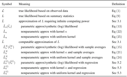
Example 4 (Synthetic likelihood for the mean of a normal distribution). The sample
average is a sufficient statistic for the task of inferring the mean θ from a sample yo =
(yo(1), . . . , yo(n)) of a normal distribution with assumed variance one. We thus reduce the
observed and simulated data yo and yθ to the empirical means Φo and Φθ, respectively,
Φo= 1
n n X
i=1
yo(i), Φθ = 1
n n X
i=1
-2 -1 0 1 2 3 4 0
10 20 30 40 50 60 70
θ
neg log synthetic likelihood
0.1, 0.9 quantiles mean
realization of stochastic process realizations at θ
(a) Negative log synthetic likelihood forN= 2
1 1.5 2 2.5
0 0.5 1 1.5 2 2.5 3 3.5 4
estimate
N = 1 N = 3 N = 10 N = ∞ (MLE)
(b) Distribution of the max synthetic likelihood estimate
Figure 2: Estimation of the mean of a Gaussian. (a) The figure shows the negative log synthetic likelihood−`ˆN
s . It illustrates that`ˆNs is a random function. (b) The randomness makes the
estimateθˇ= argmaxθ`ˆNs (θ)a random variable. Its variability increases asN decreases.
In this special case, no information is lost with the reduction to the summary statistic, that is,L(θ)∝ L(θ). Furthermore, the distribution of the summary statistic Φθ is here known,
Φθ∼ N(θ,1/n) so that the Gaussian model assumption holds and ˜Ls(θ) =L(θ).
Using for simplicity the true variance of Φθ, we have ˆ`Ns (θ) =−1/2 log(2π/n)−n/2(Φo−
ˆ
µθ)2. Since ˆµθ is an average of N realizations of Φθ, ˆµθ∼ N(θ,1/(nN)), and we can write
ˆ
`Ns as a quadratic function subject to a random shiftg,
ˆ
`Ns (θ) =−1
2log 2π
n
−n
2(Φo−θ−g)
2, g∼ N0, 1
nN
. (17)
Each realization of g yields a different mapping θ 7→ `ˆNs which illustrates that the (log) synthetic likelihood is a random function. Figure 2(a) shows the 0.1 and 0.9 quantiles of
−`ˆNs for N = 2. The dashed curve visualizes θ 7→ −`ˆNs for a fixed realization of g. The circles show values of −`ˆNs (θ) when g is not kept fixed as θ changes. The results are for sample size n= 10.
The optimizer ˇθ of each realization of ˆ`Ns depends on g, ˇθ = Φo −g. That is, ˇθ is a random variable with distribution N(Φo,1/(N n)). In the limit of an infinite amount of
available computational resources, that isN → ∞,g equals zero, and the distribution has a point-mass at ˆθmle = Φo which is indicated with the black vertical line in Figure 2(b).
As N decreases, variance is added to the point-estimate ˇθ. This added variability is due to the use of finite computational resources; it does not reflect uncertainty aboutθ due to the finite sample sizen. The variability causes an inflation of the mean squared estimation error by a factor of (1 + 1/N), E((ˇθ−θo)2) = 1/n(1 + 1/N). N
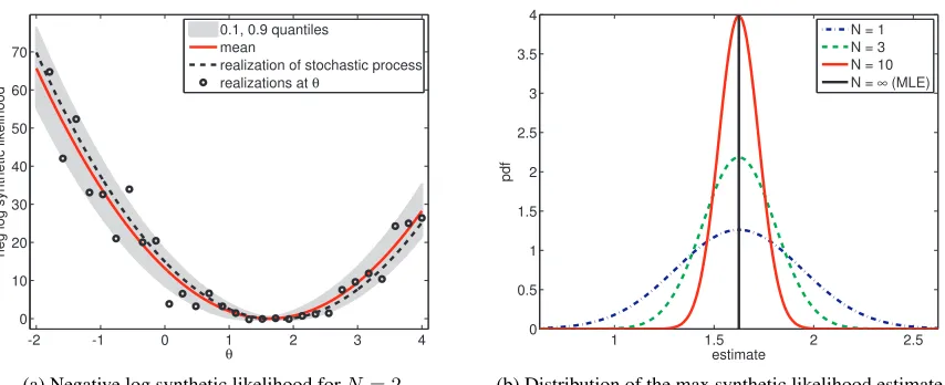
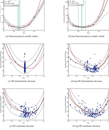
Example 5 (Synthetic likelihood for the Ricker model). Wood (2010) used the synthetic
3.2 3.4 3.6 3.8 4 4.2 10
15 20 25 30 35 40 45 50 55 60 65
log r
neg log synthetic likelihood
0.1, 0.9 quantiles, N = 50 Mean, N = 50 N = 50 N = 500 N = 5000 N = 50000
(a) Negative log synthetic likelihood for differentN
3.65 3.7 3.75 3.8 3.85 3.9 3.95
0 0.5 1 1.5
log r
neg log synthetic likelihood, offset adjusted
Mean, N = 50 N = 500 N = 5000 N = 50000
(b) Zoom forN= 500; 5,000; 50,000
Figure 3: Using less computational resources may reduce the smoothness of the approximate likeli-hood function. The figures show the negative log synthetic likelilikeli-hood−`ˆN
s for the Ricker
model. Only the first parameter (logr) was varied, the others were kept fixed at the data generating values. (a) The use of simulations makes the synthetic likelihood a stochastic process. Realizations of−`ˆNs for differentN are shown together with the variability for
N = 50. (b) The curves become more and more smooth as the numberN of simulated data sets increases even though the curve forN = 50,000is still rugged. It is reasonable to assume though that the limit forN → ∞is smooth.
complex dynamics. Time series datayθ= (y(θTb+1), . . . , y (Tb+n)
θ ) from the Ricker model after
some “burn-in” timeTbwere summarized in the form of the coefficients of the autocorrelation function and the coefficients of fitted nonlinear autoregressive models, thereby reducing the data to fourteen summary statistics Φθ (see the supplementary material of Wood, 2010, for their exact definition).
Figure 3 shows the negative log synthetic likelihood −`ˆNs for the Ricker model as a function of the log growth rate logr foryo in Figure 1(a). The parameters σ and ϕ were
kept fixed at the valuesσo = 0.3 andϕo= 10 which we used to generateyo (logrowas 3.8).
The figures show that the realizations of the synthetic likelihood become less smooth asN
decreases.
The lack of smoothness makes the minimization of the different realizations of −`ˆNs
difficult. A grid-search is feasible for very large N but this approach does not scale to higher dimensions. Gradient-based optimization is tricky because the functional form of ˆ
`Ns is unknown. Finite differences may not yield a reliable approximation of the gradient because of the lack of smoothness. Instead of optimizing a single realization of the objective, one could use an approximate stochastic gradient approach. That is, approximate gradients are computed with different random seeds at different values of the parameter. For small
3.3 Nonparametric Approximation of the Likelihood
An alternative to assuming a parametric model for the pdfpΦ|θof the summary statistics is
to approximate it by a kernel density estimate (Rosenblatt, 1956; Parzen, 1962; Mack and Rosenblatt, 1979; Wand and Jones, 1995),
pΦ|θ(φ|θ)≈EN[K(φ,Φθ)], (18)
whereK is a suitable kernel and EN denotes empirical expectation as before,
EN[K(φ,Φθ)] = 1
N N X
i=1
K(φ,Φ(θi)), Φθ(i)i.i.d.∼ pΦ|θ. (19)
An approximation of the likelihood functionL(θ) is given by ˆLNK(θ),
ˆ
LNK(θ) = EN[K(Φo,Φθ)]. (20)
We may re-write K(Φo,Φ) in another form as κ(∆θ) where ∆θ ≥ 0 depends on Φo and
Φθ, and κ is a univariate non-negative function not depending on θ. The kernels K are generally such that κ has a maximum at zero (the maximum may be not unique though). Taking the empirical expectation in Equation (20) with respect to ∆θ instead of Φθ, we have ˆLNK(θ) = ˆLNκ(θ),
ˆ
LNκ(θ) = EN[κ(∆θ)]. (21)
As the numberN grows, ˆLN
κ converges to ˜Lκ,
˜
Lκ(θ) = E [κ(∆θ)], (22)
which is ˆLNκ where the empirical average EN is replaced by the expectation E. The limiting approximate likelihood ˜Lκ(θ) does not necessarily equal the likelihood L(θ) =pΦ|θ(Φo|θ).
For example, if κ(∆θ) is obtained from a translation invariant kernel K, that is, κ(∆θ) =
K(Φo−Φθ), ˜Lκis the likelihood for a summary statistics whose pdf is obtained by convolving
pΦ|θ with K.
For convex functions κ, Jensen’s inequality yields a lower bound for ˆLNκ and its loga-rithm,
ˆ
LNκ(θ)≥κJˆN(θ), log ˆLNκ(θ)≥logκJˆN(θ), JˆN(θ) = EN[∆θ]. (23)
Since κ is maximal at zero, the lower bound is maximized by minimizing the conditional empirical expectation ˆJN(θ). The advantage of the lower bound is that it can be maximized irrespective of κ, which is often difficult to choose in practice.
A popular choice of κ for likelihood-free inference is the uniform kernel κ = κu which
yields the approximate likelihood ˆLNu ,
κu(u) =cχ[0,h)(u), LˆNu(θ) =cPN(∆θ< h), (24)
the kernel and acts as acceptance/rejection threshold. The approximate likelihood ˆLNu is proportional to the empirical probability that the discrepancy is below the threshold. The limiting approximate likelihood is denoted by ˜Lu(θ),
˜
Lu(θ) =cP (∆θ < h). (25)
The lower bound for convex κ is not applicable but we can obtain an equivalent bound by Markov’s inequality,
ˆ
LNu(θ) =ch1−PN(∆uθ ≥h)i≥c
1− 1
hE
N[∆
θ]
. (26)
The lower bound of the approximate likelihood can be maximized by minimizing ˆJN(θ) as for convex κ.
We illustrate the approximation of the likelihood via ˆLN
u in Example 6 below. It is
pointed out that good approximations are computationally very expensive because of the very small probability for ∆θ to be below small thresholdsh, or, in other words, because of the large rejection probability. We then use the model for bacterial infections in day care centers to show in Example 7 that the minimizer of ˆJN(θ) can provide a good approximation of the maximizer of ˆLNu(θ). This is important because ˆJN does not require choosing the bandwidth h or involve any rejections.
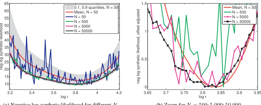
Example 6 (Approximate likelihood for the mean of a Gaussian). For the inference of
the mean of a Gaussian, we can use as discrepancy ∆θ the squared difference between the empirical mean of the observed and simulated datayoandyθ, that is the squared difference
between the two summary statistics Φo and Φθ in Example 4: ∆θ = (Φo−Φθ)2. Because of
the use of simulated data, like the synthetic likelihood, the discrepancy ∆θ is a stochastic process. We visualize its distribution in Figure 4(a). The observed datayo were the same
as in Example 4.
For this simple example, we can compute the limiting approximate likelihood ˜Lu in Equation (25) in closed form,
˜
Lu(θ)∝F
√
n(Φo−θ) +
√
nh−F√n(Φo−θ)−√nh, (27)
where F(x) is the cumulative distribution function (cdf) of a standard normal random variable,
F(x) =
Z x
−∞ 1
√
2πexp
−1
2u
2du. (28)
For small nh, ˜Lu(θ) becomes proportional to the likelihood L(θ). This is visualized in Figure 4(b).2 However, the probability to actually observe a realization of ∆
θ which is
below the thresholdh becomes vanishingly small. For realistic models, ˜Lu is not available in closed form but needs to be estimated. The vanishingly small probability indicates that the inference procedure will be computationally expensive when ˜Lu is estimated via the
sample average approximation ˆLNu. N
Example 7(Approximate univariate likelihoods for the day care centers). In the model
for bacterial infections in day care centers, the observed data were converted to summary
-2 -1 0 1 2 3 4 0
2 4 6 8 10 12 14 16
θ
discrepancy
0.1, 0.9 quantiles mean
realization of stochastic process realizations at θ
(a) Distribution of the discrepancy
0 0.5 1 1.5 2 2.5 3 3.5 4
0 0.2 0.4 0.6 0.8 1
θ
0.1, 0.9 quantiles mean threshold (0.1) approximate likelihood (rescaled) true likelihood (rescaled)
(b) Approximate likelihood
Figure 4: Nonparametric approximation of the likelihood to estimate the meanθof a Gaussian. The discrepancy∆θ is the squared difference between the empirical means of the observed
and simulated data. (a) The discrepancy is a random function. (b) The probability that the discrepancy is below some thresholdhapproximates the likelihood. Note the different range of the axes.
statistics Φo by representing each day care center (binary matrix) with four statistics. This
gives 4·29 = 116 summary statistics in total (see Numminen et al., 2013, for details). Since the day care centers can be considered to be independent, the 29 observations can be used to estimate the distribution of the four statistics and their cdfs. Numminen et al. (2013) assessed the difference between Φθand Φo by theL1 distance between the estimated
cdfs. Each L1 distance had its own uniform kernel and corresponding bandwidth, which
means that a product kernel was used overall. We here work with a simplified discrepancy measure: The different scales of the four statistics were normalized by letting the maximal value of each of the four statistics be one foryo. The discrepancy ∆θ was then theL1 norm
between Φθ and Φo divided by their dimension, ∆θ = 1/116||Φθ−Φo||1.
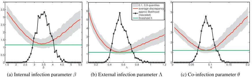
Figure 5 shows the distributions of the discrepancies ∆θ if one of the three parameters is varied at a time. The results are for the real data used by Numminen et al. (2013). The parameters were varied on a grid around the (rounded) mean (3.6,0.6,0.1) which was inferred by Numminen et al. (2013). The distributions were estimated using N = 300 realizations of ∆θ per parameter value. The red solid lines show the empirical average
ˆ
JN. The black lines with circles show ˆLNu with bandwidths (thresholds) equal to the 0.1 quantile of the sampled discrepancies. While subjective, this is a customary choice (Marin et al., 2012). The thresholds were hβ = 1.16, hΛ = 1.18, and hθ = 1.20, and are marked
with green lines. It can be seen that the optima of ˆJN and ˆLN
u are attained at about
the same parameter values which is advantageous because ˆJN is independent of kernel and bandwidth.
1.5 2 2.5 3 3.5 4 4.5 5 5.5 0
0.5 1 1.5 2 2.5 3 3.5 4
β
(a) Internal infection parameterβ
0.2 0.4 0.6 0.8 1 1.2
0 1 2 3 4 5 6 7
Λ
0.1, 0.9 quantiles average discrepancy approx likelihood (rescaled) threshold h
(b) External infection parameterΛ
0 0.05 0.1 0.15 0.2
0 1 2 3 4 5 6
θ
(c) Co-infection parameterθ
Figure 5: Approximate likelihoods LˆNu and distributions of the discrepancy ∆θ for the day care center example. The green horizontal lines indicate the thresholds used. The optima of the average discrepancies and the approximate likelihoods occur at about the same parameter values.
combining probabilistic modeling with optimization, which we mentioned in Example 5 for
the log synthetic likelihood, is also helpful here. N
3.4 Relation between Nonparametric and Parametric Approximation
Kernel density estimation with Gaussian kernels is interesting for two reasons in the context of likelihood-free inference. First, the Gaussian kernel is positive definite, so that the estimated density is a member of a reproducing kernel Hilbert space. This means that more robust approximations ofpΦ|θ than the one in Equation (18) would exist (Kim and Scott,
2012), and that there might be connections to the inference approach of Fukumizu et al. (2013). Second, it allows us to embed the synthetic likelihood approach of Section 3.2 into the nonparametric approach of Section 3.3.
For the Gaussian kernel, we have that K(Φo,Φθ) =Kg(Φo−Φθ),
Kg(Φo−Φθ) =
1 (2π)p/2
1
|detCθ|1/2
exp −(Φo−Φθ) >C−1
θ (Φo−Φθ)
2
!
, (29)
whereCθ is a positive definite bandwidth matrix possibly depending on θ. The kernelKg
corresponds to κ=κg and ∆θ= ∆gθ,
κg(u) = 1
(2π)p/2exp
−u
2
, ∆gθ= log|detCθ|+ (Φo−Φθ)>C−θ1(Φo−Φθ). (30)
The functionκg is convex so that Equation (23) yields a lower bound for ˆLN(θ) = ˆLNg (θ) and its logarithm,
log ˆLNg (θ)≥ −p
2log(2π)− 1 2
ˆ
JgN(θ), (31)
ˆ
JgN(θ) = ENhlog|detCθ|+ (Φo−Φθ)>C−θ1(Φo−Φθ)
i
We used the subscript “g” to highlight that ˆJN in Equation (23) is computed for the particular discrepancy ∆gθ. The form of ˆJgN is reminiscent of the log synthetic likelihood ˆ`Ns
in Equation (15). The following proposition shows that there is indeed a connection.
Proposition 1(Synthetic likelihood as lower bound). ForCθ=Σˆθ,
ˆ
`Ns (θ) = p 2−
p
2log(2π)− 1 2
ˆ
JgN(θ), (33)
log ˆLNg (θ)≥ −p
2 + ˆ`
N
s (θ) (34)
The proposition is proved in Appendix A. It shows that maximizing the synthetic log-likelihood corresponds to maximizing a lower bound of a nonparametric approximation of the log likelihood. The proposition embeds the parametric approach to likelihood ap-proximation conceptually in the nonparametric one and shows furthermore that ˆ`Ns can be computed via an empirical expectation over ∆gθ.
3.5 Posterior Inference using Sample Average Approximations of the Likelihood
Several computable approximations ˆL of the likelihoodL were constructed in the previous two sections. Table 1 provides an overview. Intractable expectations were replaced with sample averages usingN simulated data sets which we denoted by the superscript “N” in the symbols for the approximations.
Wood (2010) used the synthetic likelihood ˆLNs together with a Metropolis MCMC al-gorithm for posterior computations. We here focus on posterior inference via importance sampling. Using ˆLNu as ˆL in Equation (11), we have
E(g(θ)|Φo)≈ M X
m=1
g(θ(m)) ˆwu(m), wˆu(m)=
PN
j=1χ[0,h)(∆
(jm)
θ )
pθ(θ(m))
q(θ(m))
PM
i=1
PN
j=1χ[0,h)(∆
(ji) θ )
pθ(θ(i))
q(θ(i))
, (35)
where χ[0,h) is the indicator function of the interval [0, h) as before, and the ∆(θjm), j =
1, . . . , N,are the observed discrepancies for the sampled parameterθ(m)∼q(θ). Instead of
sampling several discrepancies for the sameθ(m), samplingM0 pairs (∆θ(i),θ(i)) withN = 1 is also possible and corresponds to an asymptotically equivalent solution. Withq=pθ, the
approximation is a Nadaraya–Watson kernel estimate of the conditional expectation (see, for example, Wasserman, 2004, Chapter 21).
Approximate Bayesian computation (ABC) is intrinsically linked to kernel density es-timation and kernel regression (Blum, 2010). A basic ABC rejection sampler (Pritchard et al., 1999; Marin et al., 2012, Algorithm 2) is obtained from Equation (35) with N = 1,
q = pθ, and ∆θ = ||Φo −Φθ|| where ||.|| is some norm. Approximate samples from the
posterior pdf ofθ given Φo can thus be obtained by retaining thoseθ(m)for which the Φ(θm)
are within distancehfrom Φo. In an iterative approach, the accepted particles can be used
to define the auxiliary pdfq(θ) of the next iteration by letting it be a mixture of Gaussians with weights ˆw(um), center pointsθ(m), and a covariance determined by theθ(m) (Beaumont
by Sisson et al. (2007) and Toni et al. (2009). Working withq=pθ, Beaumont et al. (2002)
introduced ABC with more general kernels, which corresponds to using ˆLNκ instead of ˆLNu. Example 6 showed that approximating the likelihood via sample averages is computa-tionally expensive because of the required small thresholds. The auxiliary pdfq(θ) specifies where in the parameter space the likelihood is predominantly evaluated. The following ex-ample shows that avoiding regions in the parameter space where the likelihood is vanishingly small allows for considerable computational savings.
Example 8(Univariate approximate posteriors for the day care centers). For the inference
of the model of bacterial infections in day care centers, Numminen et al. (2013) used uniform priors for the parametersβ ∈(0,11), Λ∈(0,2), and θ∈(0,1). The likelihoods ˆLNu shown in Figure 5 are thus proportional to the posterior pdfs. The posterior pdfs of the univariate unknowns are conditional on the remaining fixed parameters. For example, the posterior pdf forβ is conditional on (Λ, θ) = (Λo, θo) = (0.6,0.1). In Section 7, we consider inference of all three parameters at the same time.
In Figure 5, each parameter is evaluated on a sub-interval of the domain of the prior. The sub-intervals were chosen such that the far tails of the likelihoods were excluded. Parameter
β, for example, was evaluated on the interval (1.5,5.5) only. Evaluating the discrepancy ∆θ on the complete interval (0,11) is not very meaningful since the probability that it is above the chosen threshold is vanishingly small outside the interval (1.5,5.5). In fact, out of M = 5,000 discrepancies ∆θ which we simulated forβ uniformly on (0,11), not a single one was accepted for β /∈ (1.5,5.5). Hence, taking for instance a uniform distribution on (1.5,5.5) instead of the prior as auxiliary distribution leads to considerable computational savings. Motivated by this, we propose a method which automatically avoids regions in the
parameter space where the likelihood is vanishingly small. N
4. Computational Difficulties in the Standard Inference Approach
We have seen that the approximate likelihood functions ˆL(θ) which are used to infer simulator-based statistical models are stochastic processes indexed by the model param-eters θ. Their properties, in particular their functional form and gradients, are generally not known; they behave like stochastic black-box functions. The stochasticity is due to the use of simulations to approximate intractable expectations. In the standard approach presented in the previous section, the expectations are approximated by sample averages so that a single evaluation of ˆLrequires the simulation ofN data sets. The standard approach makes minimal assumptions but suffers from a couple of limiting factors.
1. There is an inherent trade-off between computational and statistical efficiency: Re-ducing N reduces the computational cost of the inference methods, but it can also decrease the accuracy of the estimates (Figure 2).
2. For finiteN, the approximate likelihoods may not be smooth (Figure 3).
5. Framework to Increase the Computationally Efficiency
We present a framework which combines optimization with probabilistic modeling in order to increase the efficiency of likelihood-free inference of simulator-based statistical models.
5.1 From Sample Average to Regression Based Approximations
The standard approach to obtain a computable approximate likelihood function ˆL relies on sample averages, yielding the parametric approximation ˆLNs = exp(ˆ`Ns ) in Equation (15) or the nonparametric approximation ˆLNκ in Equation (21). The approximations are computable versions of ˜Ls = exp(˜`s) in Equation (13) and ˜Lκ in Equation (22), which both
involve intractable expectations. But sample averages are not the only way to approximate the intractable expectations. We here consider approximations based on regression.
Equation (22) shows that ˜Lκ(θ) has a natural interpretation as a regression function
where the model parameters θ are the covariates (the independent variables) andκ(∆θ) is
the response variable. The expectation can thus also be approximated by solving a regression problem. Further, ˆJN in Equation (23) can be seen as the sample average approximation of the regression function J(θ),
J(θ) = E [∆θ], (36)
where the discrepancy ∆θ is the response variable. The arguments which we used to show that ˆJN provides a lower bound for ˆLNκ carry directly over toJ and ˜Lκ: J provides a lower bound for ˜Lκ ifκ is convex or the uniform kernel.
Proposition 1 establishes a relation between the sample average quantities ˆJN
g in
Equa-tion (32) and ˆ`Ns in Equation (15). In the proof of the proposition in Appendix A, we show that the relation extends to the limiting quantitiesJg(θ) = E
∆gθ
and ˜`s in Equation (13).
Thus, for Cθ = Σθ and up to constants and the sign, ˜`s(θ) can be seen as a regression
function with the particular discrepancy ∆gθ as the response variable.
We next discuss the general strategy to infer the regression functions while avoiding unnecessary computations. For nonparametric approximations to the likelihood, inferring
J is simpler than inferring ˜Lκ since the function κ and its corresponding bandwidth do not need to be chosen. We thus propose to first infer the regression function J of the discrepancies and then, in a second step, to leverage the obtained solution to infer ˜Lκ. For the parametric approximation to the likelihood, this extra step is not needed since Jg is a special instance of the regression function J.
5.2 Inferring the Regression Function of the Discrepancies
Inferring J(θ) via regression requires training data in the form of tuples (θ(i),∆(θi)). Since we are mostly interested in the region of the parameter space where ∆θ tends to be small, we propose to actively construct the training data such that they are more densely clustered around the minimizer ofJ(θ). AsJ(θ) is unknown in the first place, our proposal amounts to performing regression and optimization at the same time: Given an initial guess that the minimizer is in some bounded subset of the parameter space, we can sample some evidence
E(t) of the relation betweenθ and ∆ θ,
and use this evidence to obtain an estimate ˆJ(t) ofJ via regression. The estimated ˆJ(t) and
some measurement of uncertainty about it can then be used to produce a new guess about the potential location of the minimizer, from where the process re-starts. In some cases, it may be advantageous to include the prior pdf of the parameters in the process. We explore this topic in Appendix B.
The evidence set E(t) grows at every iteration and we may stop att=T. The value of
T can be chosen based on computational considerations, by checking whether the learned model predicts the acquired points reasonably well, or by monitoring the change in the
minimizerθˆ(Jt) of ˆJ(t) as the evidence set grows,
ˆ
θ(Jt)= argminθJˆ(t)(θ). (38)
Given our examples so far, it is further reasonable to assume that J is a smooth func-tion. Even for the Ricker model, the mean objective was smooth although the individual realizations were not (Figure 3). The smoothness assumption about J can be used in the regression and enables its efficient minimization.
For the special case where ˜`s is the target, several observed values of ∆θ = ∆gθ may
be available for any given θ(i). This is because the covariance matrix Σθ may be still
estimated as a sample average so that multiple simulated summary statistics, and hence discrepancies, are available per θ(i). They can be used as discussed above with the only minor modification that the training data are updated with several tuples at a time. But it is also possible to only use the average value of the observed discrepancies, which amounts to using the observed values of ˆ`N
s for training. The estimated regression function ˆJ(t)provides
an estimate for ˜`s in either case. We denote the estimate by ˆ`(st) and the corresponding
estimate of ˜Ls by ˆL(st).
Combining nonlinear regression with the acquisition of new evidence in order to optimize a black-box function is known as Bayesian optimization (see, for example, Brochu et al., 2010). We can thus leverage results from Bayesian optimization to implement the proposed approach, which we will do in Section 6.
5.3 Inferring the Regression Function for Nonparametric Likelihood Approximation
The evidence set E(t) can be used in two possible ways in the nonparametric setting: The
first possibility is to compute for each ∆(θi) inE(t) the value κ(i) =κ(∆(i)
θ ) and to thereby
produce a new evidence set which can be used to approximate ˜Lκ by fitting a regression function. The second possibility is to estimate a probabilistic model of ∆θfrom the evidence
E(t). The estimated model can be used to approximate ˜L
κ by replacing the expectation in
Equation (22) with the expectation under the model. We denote either approximation by ˆ
L(κt)where the superscript “(t)” indicates that the approximation was obtained via regression
witht training points. SinceE(t) is such that the approximation of the regression function
is accurate where it takes small values, the approximation of ˜Lκ will be accurate where it
takes large values, that is, in the modal areas.
see, for example, Wand and Jones, 1995). The results from that literature are, however, not straightforwardly applicable to our work: We may only be given a certain discrepancy measure ∆θ without underlying summary statistics Φθ (Gutmann et al., 2014). And even if the discrepancy ∆θ is constructed via summary statistics, the kernel density estimate is only evaluated at Φo which is kept fixed while θ is varied. Furthermore, we usually only
have very few observations available for any givenθ which is generally not the case in kernel density estimation. These differences warrant further investigations into which extent the bandwidth selection methods from the kernel density estimation literature are applicable to likelihood-free inference. We focus in this paper on the uniform kernel and generally choose h via the quantiles of the ∆(θi), which is common practice in approximate Bayesian computation (see, for example, Marin et al., 2012). The approximate likelihood function for the uniform kernel will be denoted by ˆL(ut).
5.4 Benefits and Limitations of the Proposed Approach
The difference between the proposed approach and the standard approach to likelihood-free inference of simulator-based statistical models lies in the way the intractable J and
˜
L are approximated. We use regression with actively acquired training data while the standard approach relies on computing sample averages. Our approach allows to incorporate a smoothness assumption about J and ˜L in the region of their optima. The smoothness assumption allows to “share” observed ∆θ among multiple θ which suggests that fewer
∆(θi), that is, fewer simulated data setsy(θi), are needed to reach a certain level of accuracy. A second benefit of the proposed approach is that it directly targets the region in the parameter space where the discrepancy ∆θ tends to be small, which is very important if
simulating data sets is time consuming.
Regression and deciding on the training data are not free of computational cost. While the additional expense is often justified by the net savings made, it goes without saying that if simulating the model is very cheap, methods for regression and decision making need to be used which are not disproportionately costly. Furthermore, prioritizing the low-discrepancy areas of the parameter space is often meaningful, but it also implies that the tails of the likelihood (posterior) will not be as well approximated as the modal areas. The proposed approach thus had to be modified if the computation of small probability events was of primary interest.
Section 4 lists three computational difficulties occurring in the standard approach. Our approach addresses the smoothness issues via smooth regression. The inefficient use of resources is addressed by focusing on regions in the parameter space where ∆θ tends to be small. The trade-off between computational and statistical performance is still present but in modified form: The trade-off is the size of the training set E(t) used in the regression.
6. Implementing the Framework with Bayesian Optimization
We start with introducing Bayesian optimization and then use it to implement our frame-work. This is followed by a discussion of possible extensions.
6.1 Brief Introduction to Bayesian Optimization
We briefly introduce the elements of Bayesian optimization which are needed in the paper. A more thorough introduction can be found in the review articles by Jones (2001) and Brochu et al. (2010). While the presented version of Bayesian optimization is rather straightforward and textbook-like, our framework can also be implemented with more advanced versions, see Section 6.4.
Bayesian optimization comprises a set of methods to minimize black-box functionsf(θ). With a black-box function, we mean a function which we can evaluate but whose form and gradients are unknown. The basic idea in Bayesian optimization is to use a probabilistic model of f to select points where the objective is evaluated, and to use the obtained values to update the model by Bayes’ theorem.
The objectivef is often modeled as a Gaussian process which is also done in this paper: We assume that f is a Gaussian process with prior mean function m(θ) and covariance functionk(θ,θ0) subject to additive Gaussian observation noise with varianceσn2. The joint distribution of f at anyt pointsθ(1), . . . ,θ(t) is thus assumed Gaussian with meanmt and
covarianceKt,
f(1), . . . , f(t)>∼ N(mt,Kt), (39)
mt=
m(θ(1)) .. .
m(θ(t))
, Kt=
k(θ(1),θ(1)) . . . k(θ(1),θ(t)) ..
. ...
k(θ(t),θ(1)) . . . k(θ(t),θ(t))
+σ2nIt. (40)
We usedf(i) to denotef(θ(i)) and It is thet×t identity matrix. While other choices are
possible, we assume that m(θ) is either a constant or a sum of convex quadratic polyno-mials in the elements θj ofθ, cross-terms were not included, and that k(θ,θ0) is a squared exponential covariance function,
m(θ) =X
j
ajθ2j +bjθj+c, k(θ,θ0) =σf2exp
X
j
1
λ2j(θj−θ 0
j)2
. (41)
These are standard choices (see, for example, Rasmussen and Williams, 2006, Chapter 2). Since we are interested in minimization, we constrain the aj to be non-negative. In
the last equation, θj and θ0j are the elements of θ and θ0, respectively, σf2 is the signal variance, and the λj are the characteristic length scales. The length scales control the
amount of correlation between f(θ) and f(θ0), in other words, they control the wiggliness of the realizations of the Gaussian process. The signal variance is the marginal variance of
f at a point θ if the observation noise was zero.
of cross-validation, see Rasmussen and Williams, 2006, Section 5.4.2). The hyperparameters were slowly updated as new data were acquired, as done in previous work, for example by Wang et al. (2013). This yielded satisfactory results but there are several alternatives, including Bayesian methods to learn the hyperparameters (for an overview, see Rasmussen and Williams, 2006, Chapter 5), and we did not perform any systematic comparison.
Given evidence Ef(t) = {(θ(1), f(1)), . . . ,(θ(t), f(t))}, the posterior pdf of f at a point θ
is Gaussian with posterior meanµt(θ) and posterior variancevt(θ) +σn2,
f(θ)|Ef(t)∼ N(µt(θ), vt(θ) +σn2), (42)
where (see, for example, Rasmussen and Williams, 2006, Section 2.7),
µt(θ) =m(θ) +kt(θ)>K−t1(ft−mt), vt(θ) =k(θ,θ)−kt(θ)>K−t1kt(θ), (43)
ft= f(1), . . . , f(t) >
, kt(θ) = k(θ,θ(1)), . . . , k(θ,θ(t))
>
. (44)
The posterior mean µt emulates f and can be minimized with powerful gradient-based optimization methods.
The evidence set can be augmented by selecting a new point θ(t+1) where f is next evaluated. The point is chosen based on the posterior distribution of f given Ef(t). While other choices are equally possible, we use the acquisition function At(θ) to select the next
point,
At(θ) =µt(θ)− q
η2tvt(θ), (45)
whereη2t = 2 log[td/2+2π2/(3η)] withη being a small constant (we usedη = 0.1). This
ac-quisition function is known as the lower confidence bound selection criterion (Cox and John, 1992, 1997; Srinivas et al., 2010, 2012).3 Classically,θ(t+1)is chosen deterministically as the minimizer of At(θ). The minimization of At(θ) yields a compromise between exploration and exploitation: Minimization of the posterior meanµt(θ) corresponds to exploitation of the current belief and ignores its uncertainty. Minimization of−p
vt(θ), on the other hand, corresponds to exploration where we seek a point where we are uncertain about f. The coefficientηt implements the trade-off between these two desiderata.
There is usually no restriction that θ(t+1) must be different from previously acquired
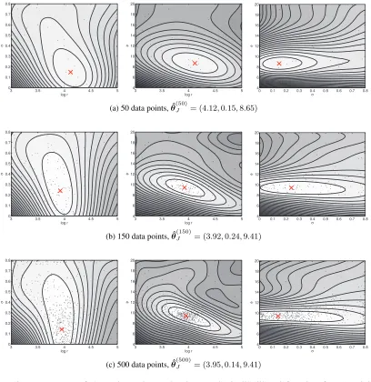
θ(t). We found, however, that this may result in a poor exploration of the parameter space (see Figure 7 and Example 10 below). Employing a stochastic acquisition rule avoids getting stuck at one point. We used the simple heuristic thatθ(t+1)is sampled from a Gaussian with diagonal covariance matrix and mean equal to the minimizer of the acquisition function. The standard deviations were determined by finding the end-points of the interval where the acquisition function was within a certain (relative) tolerance. Other stochastic acquisition rules, like for example Thompson sampling (Thompson, 1933; Chapelle and Li, 2011; Russo and Van Roy, 2014), could alternatively be used.
The algorithm was initialized with an evidence setE(t0)
f where the parametersθ
(1), . . . ,θ(t0)
were chosen as a Sobol quasi-random sequence (see, for example, Niederreiter, 1988). Com-pared to uniformly distributed (pseudo) random numbers, the Sobol sequence covers the
3. In the literature, maximization instead of minimization problems are often considered. For maximization problems, the acquisition function becomesµt(θ) +
p
η2
tvt(θ)and needs to be maximized. The formula forη2t is used in the