Benefitting from the Variables that Variable Selection Discards
Rich Caruana [email protected]
Computer Science Department Cornell University
Ithaca, NY 14853, USA
Virginia R. de Sa [email protected]
Department of Cognitive Science University of California, San Diego La Jolla, CA 92093-0515, USA
Editors: Isabelle Guyon and Andr´e Elisseeff
Abstract
In supervised learning variable selection is used to find a subset of the available inputs that accurately predict the output. This paper shows that some of the variables that variable selection discards can beneficially be used as extra outputs for inductive transfer. Using discarded input vari-ables as extra outputs forces the model to learn mappings from the varivari-ables that were selected as inputs to these extra outputs. Inductive transfer makes what is learned by these mappings available to the model that is being trained on the main output, often resulting in improved performance on that main output.
We present three synthetic problems (two regression problems and one classification problem) where performance improves if some variables discarded by variable selection are used as extra outputs. We then apply variable selection to two real problems (DNA splice-junction and pneumo-nia risk prediction) and demonstrate the same effect: using some of the discarded input variables as extra outputs yields somewhat better performance on both of these problems than can be achieved by variable selection alone. This new approach enhances the benefit of variable selection by al-lowing the learner to benefit from variables that would otherwise have been discarded by variable selection, but without suffering the loss in performance that occurs when these variables are used as inputs.
Keywords: multitask learning, output variable selection, inductive transfer
1. Introduction
The goal of supervised learning is to learn functions that map inputs to outputs. In high-dimensional problems with finite training data, using all available variables as inputs usually is suboptimal. Most algorithms learn better given a carefully selected subset of variables to use as inputs (Caruana and Freitag, 1994, John et al., 1994, Koller and Sahami, 1996). If variable selection is used to find the subset of variables to use as inputs, what should be done with the variables not selected? Usually, variables not selected as inputs are discarded. Instead of discarding variables not selected by variable selection for use as inputs, can we benefit from the information they contain some other way?
outputs. Methods for doing this include hints (Abu-Mostafa, 1989), tangent-prop (Simard et al., 1992), EBNN (Thrun and Mitchell, 1994), and multitask learning (Caruana, 1997a). In unsuper-vised learning, de Sa’s minimizing disagreement algorithm (de Sa, 1994, de Sa and Ballard, 1998) and Becker’s IMAX (Becker and Hinton, 1989) use features arising from another modality to derive an output to help the other modality learn.
In this paper we concentrate on the multitask learning (MTL) method of giving extra information through the model’s outputs. In multitask learning, extra outputs are trained in parallel with the main task output(s) while using a shared representation. For example, in a backprop net (Rumelhart et al., 1986), multitask learning is implemented by having extra outputs share a common hidden layer in the network with the main task output(s). This sharing promotes inductive transfer: the hidden layer representations learned for the extra outputs are available to the main task output(s) and often improve performance on the main task. MTL in backprop nets is well documented (Suddarth and Holden, 1991, Abu-Mostafa, 1989, Baxter, 1995, Caruana, 1995, Dietterich et al., 1995, Ghosn and Bengio, 1997, Caruana, 1997a,b).
MTL often is used to benefit from information available in the training set that can not be used as inputs because it will not be available for future test cases (Caruana, 1996). For example, in medicine, it may take several days to get back the results of some lab tests, but a decision must be made about how to start treating the patient before those test results will be available. The lab test results are available for the patients in the training set, but will not be available when making predictions for new patients. Variables such as these can’t be used as standard inputs because they will be missing when making predictions. Instead of ignoring them, MTL gets the inductive transfer benefit from them by using them as extra outputs (Baluja and Pomerleau, 1995, Caruana, 1995).
The good results from MTL led us to ask: If variables that can’t be used as inputs (e.g., because they will be missing) are useful as extra outputs, might some of the inputs that variable selection dis-cards also be useful as extra outputs? In this paper we show preliminary results to this question. In supervised back-propagation learning, there are problems where variables that harm performance as
inputs can improve performance as outputs. This demonstration is first made on problems carefully
engineered to demonstrate this effect. For these problems variable selection is not needed because we know which variables might be more useful as extra outputs than as inputs.
We then show results from two real problems where inputs discarded by variable selection pro-vide additional benefit when used as extra outputs. We show that the DNA splice-junction domain contains variables that yield somewhat better recognition accuracy when used as extra outputs than when used as inputs (where they are in fact harmful). We use the variable selection method devel-oped by Koller and Sahami (1996) to select which variables to use as inputs. They showed naive bayes and C4.5 achieve better accuracy using just the selected variables as inputs than using all the variables as inputs. We show a similar result for backprop nets. We then show that it is better to use some of the variables not used as inputs as extra outputs instead of ignoring them. Best performance is achieved by moving some of the input variables to the output side of the net. We show stronger results on a pneumonia risk prediction problem. On that problem variable selection improves the performance of a backprop net compared to a net trained using all of the available inputs. But a net that uses some of the discarded variables as extra outputs performs even better.
benefit might be achieved if we are able to develop variable selection methods that efficiently select both inputs and extra outputs at the same time, and are currently working to develop such meth-ods. The results in this paper should be viewed more as a proof of concept, than as the final word in this area. One reason why we are excited by this research despite the modest performance im-provements is that we suspect many real world problems will benefit from a similar combination of variable selection and multitask learning.
MTL originally was formulated to take advantage of variables available in the training data, but not available in the test data. Variable selection is important for most practical, data-limited, machine learning problems where it is beneficial to reduce the search space. In this paper we combine these two ideas. If training data is limited and it is necessary to reduce the search space by restricting the number of input variables, it is not necessary to ignore the variables not selected as inputs. Using them as extra outputs, as in MTL, is one way to benefit from them without paying the penalty of increasing the dimensionality of the search space. The main difference between this use of MTL and the original applications of MTL is that in this case we could use the variables as inputs but choose to use them as extra outputs instead in order to improve performance.
MTL is a form of inductive transfer that is applicable to any learning method that can share part of what is learned between multiple tasks. See Section 5 for a brief discussion of how variable selection and MTL could be used with other learning methods such as k-nearest neighbor (kNN) and Support Vector Machines (SVMs). In this paper we demonstrate the combination of variable selection and MTL with the backpropagation1algorithm (Rumelhart et al., 1986). In backprop nets, it is a hidden layer shared by the outputs on the net that allows inductive transfer to occur between the outputs.
This paper uses the following terms: The Main Task is the output to be learned. Anything that improves performance on the Main Task is good. Selected Inputs are the variables provided as inputs in all experiments. Extra Inputs are the extra variables (selected from the discarded variables) when used as inputs. Extra Outputs are the same extra variables (from the discarded variables) when they are used as outputs (instead of as inputs). STD is standard backpropagation using the Selected Inputs as inputs and only the Main Task as outputs. This is the standard way of doing backpropagation learning after variable selection. STD+IN uses the Extra Variables as Extra Inputs to learn the Main Task. STD+OUT uses the Extra Variables, but as Extra Outputs learned in parallel with the Main Task, using just the Selected Inputs as inputs.
2. Synthetic Problems
In this section we show, by using constructed problems, why variables used as extra outputs can be more useful than those same variables used as extra inputs. In this section variable selection is largely trivial.
2.1 Poorly Correlated Variables
This section presents a simple synthetic problem where using a variable as an extra output is better than using that same variable as an extra input. We present this problem first because it is easy to see why the variable is not useful as an input, but is useful as an extra output.
Consider the following function:
F1(A,B) =SIGMOID(A+B), SIGMOID(x) =1/(1+e(−x))
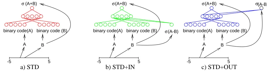
Now consider the STD net shown in Figure 1a with 20 inputs, 16 hidden units (fewer input and hidden units are shown in the figure for clarity), and one output. We use backpropagation on this net to Learn the function F1(·).
Data is generated by randomly sampling values A and B uniformly from the interval [-5,5], and then computing the SIGMOID of their sum. The network input receives a binary coded version of A and B. The range [-5,5] is discretized into 210bins and the binary encoding of the resulting bin number is used as the input coding. The first 10 input units receive this coding for A and the second 10 that for B. The target output for the 20 bit encoding of A and B is the unary real (unencoded) value F1(A,B).
(A+B)
5
A B
-5
binary code(A) binary code (B) σ
(A-B)
5
A B
-5
binary code(A) binary code (B) (A+B)
σ
σ
(A-B)
5
A B
-5
binary code(A) binary code (B) (A+B)
σ σ
a) STD b) STD+IN c) STD+OUT
Figure 1: Three Neural Net Architectures for Learning F1.
Backpropagation is done with per-epoch updating and early stopping. For each trial, we generate new random training, halt, and test sets. Training sets contain 50 patterns. This is enough data to get good performance, but not so much that there is not room for improvement. We use large halt and test sets — 1000 cases each — to minimize the effect of sampling error in the measured performances. Larger halt and test sets yield nearly identical results. We use this methodology for all the experiments on synthetic problems.
Table 1 shows the mean performance of 50 trials of STD Net 1a with backpropagation and early stopping.
Network Trials Mean RMSE Significance
STD 50 0.0648
-STD+IN 50 0.0647 ns
STD+OUT 50 0.0631 0.013*
Table 1: Mean Test Set Root-Mean-Squared-Error on F1.
Now consider the similar function:
F2(A,B) =SIGMOID(A−B).
Probably not. A+B and A-B do not correlate for random A and B. The correlation coefficient of A+B to A-B for our training sets is typically less than 0.01. Because of this, knowing the value of F2(A,B) does not tell you much about the target value F1(A,B) (and vice-versa).
The fact that F1(A,B) does not correlate well with F2(A,B) hurts backprop’s ability to learn to use F2(A,B) to predict F1(A,B). The net in Figure 1b has 21 inputs — 20 for the binary code for A and B, and an extra input for F2(A,B). The 2nd line in Table 1 shows the performance of STD+IN for the same training, halting, and test sets used by STD; the only difference is that there is an extra input variable in the data sets for STD+IN. A t-test shows that the performance of STD+IN is not significantly different from that of STD even with 50 trials — the extra information contained in the variable F2(A,B) does not help backpropagation learn F1(·)when used as an extra input.
If using F2(A,B) as an extra input does not help backpropagation learn F1(·), should we ignore
F2(·) altogether? No. Functions F 1(·) and F2(·) are strongly related. They both need to learn to compute the same subvariables, A and B from the binary coded inputs. If, instead of using F2(A,B) as an extra input, it is used as an extra output that must be learned via backpropagation, it will bias the shared hidden layer to learn A and B better, and this will help the net better learn to predict
F1(·).
Figure 1c shows a net with 20 inputs for A and B, and 2 outputs, one for F1(A,B) and one for F2(A,B). The performance of this net is evaluated only on the output F1(A,B), but backpropagation is done on both outputs. The 3rd line in Table 1 shows the mean performance of 50 trials of this
multitask net on F1(·). Early stopping is done by examining only the performance at the output
for F 1(·). Using F2(A,B) as an extra output on a net also learning F1(·) significantly improves performance on F1(·). Using the extra variable as an extra output is better than using it as an extra
input. By using F2(A,B) as an output we make use of more than just the individual output values F2(A,B) but can extract information about the function mapping F2(·)itself. This is a key difference between using variables as inputs and outputs.
The increased performance of STD+OUT over STD and STD+IN is not due to STD+OUT restricting the capacity available in the net for the main task F1. All three nets — STD, STD+IN, STD+OUT — perform better when given more than 16 hidden units. In fact, if we double the number of hidden units in the STD+OUT net to 32, the larger STD+OUT net does even better (We report the results for the 16 hidden unit STD net to be fair to STD and STD+IN).
2.2 Noisy Variables
This section presents two problems where the extra variables are more useful as inputs if the noise added to them is small, but which become more useful as outputs as the noise increases. Because the extra variables are ideal variables for these problems, this demonstrates that the effect observed in the previous section does not depend on the extra variables being contrived so that their correlation with the main task is low – variables with high correlation can still be more useful as outputs if they are noisy.
Once again, consider the main task from the previous section:
F1(A,B) =SIGMOID(A+B).
Now consider these extra variables:
Noise is independent uniformly sampled noise on [-1,1]. If the noise scale is not too large,
EF(A) and EF(B) are excellent input variables for learning F1(·) because the network no longer
needs to learn to decode the binary input representation. However, as the noise scale increases, EF(A) and EF(B) become less useful and it is better for the net to learn F1(·)from the binary inputs for A and B.
As before, we consider using the extra variables as either extra inputs or as extra outputs. The goal is to learn F1(·) from random training sets of size 50, and the halt and test sets have 1000 patterns. Here we use nets with 256 hidden units, because preliminary experiments showed 256 hidden units to be the smallest net that performs near optimally on this problem.
0.044 0.046 0.048 0.05 0.052 0.054 0.056 0.058 0.06
0 2 4 6 8 10
Test Set RMSE
Feature Noise Scale
STD STD+IN
STD+OUT
0.12 0.13 0.14 0.15 0.16 0.17 0.18
0 2 4 6 8 10
Test Set RMSE
Feature Noise Scale
STD STD+IN
STD+OUT
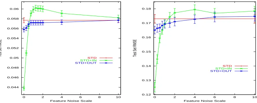
Figure 2: STD, STD+IN, and STD+OUT on F1 (left) and F3 (right). Error bars are±one standard
error.
Figure 2 (left) plots the average performance of 20 trials of STD+IN and STD+OUT as the noise scale is varied from 0.0 to 10.0. The performance of STD, which does not use EF(A) and EF(B), is shown as a horizontal line; it is independent of the noise scale. Let’s first examine the results of STD+IN which uses EF(A) and EF(B) as extra inputs. As expected, when the noise is small, using EF(A) and EF(B) as extra inputs improves performance considerably. As the noise increases, however, this improvement decreases. Eventually, there is so much noise in EF(A) and EF(B) that they no longer help the net if used as inputs. And, if the noise increases further, using EF(A) and EF(B) as extra inputs actually hurts. Finally, as the noise gets very large, performance asymptotes back towards the baseline. This is because when the noise is very large the net learns to ignore the extra variables altogether.
The results of using EF(A) and EF(B) as extra outputs are quite different. When the noise is low, the extra outputs do not help as much as the extra inputs. As the noise increases, however, the benefit from the extra outputs decreases more slowly than with the extra inputs. Because of this, at some point the extra outputs help more than the extra inputs. Furthermore, as the noise increases, the extra outputs never hurt performance the way the extra inputs did.
the extent that the main task is a function of the noisy inputs, it must pass the noise in these to the output. This causes the output to be noisy. Also, as the net comes to depend on the noisy inputs, it depends less on the noise-free binary inputs. In other words, if the noisy inputs explain away some of the training samples, fewer training samples are left to encourage learning to decode the binary inputs.
Why does noise not hurt STD+OUT as much as it hurts STD+IN? As an output, the net is learning the mapping from the regular inputs to EF(A) and EF(B). Early in training, the net learns to interpolate through the noise and thus learns smooth functions for EF(A) and EF(B) that have reasonable fidelity to the true mapping. This makes learning less sensitive to the noise added to these variables.
2.2.1 ANOTHER PROBLEM
F1(·) is only mildly nonlinear because the interval that A and B are defined on does not often go far into the tails of the SIGMOID. Do the results with noisy variables depend on this smoothness? To check this, we modified F1(·)to make it much more nonlinear. Consider this function:
F3(A,B) =SIGMOID(EX PAND(SIGMOID(A)− −SIGMOID(B)))
where EXPAND scales the inputs from (SIGMOID(A)–SIGMOID(B)) to the range [-12.5,12.5], and A and B are drawn from [-12.5,12.5]. F3(·)is significantly more nonlinear than F1(·)because the expanded ranges of A and B, and expanding the difference to [-12.5,12.5] before passing it through another sigmoid, cause much of the data to fall in the tails of either one of the first layer sigmoids or the final sigmoid.
Consider these extra variables:
EF(A) =SIGMOID(A) +SCALE∗Noise
EF(B) =SIGMOID(B) +SCALE∗Noise
where Noise is sampled as before. Figure 2 (right) shows the results of using extra variables EF(A) and EF(B) as extra inputs and as extra outputs. The trend is similar to that in Figure 2 (left) but the benefit of STD+OUT is even larger at low noise. Note that the data for both figures are generated using different seeds, for the left figure we used steepest descent and Mitre’s Aspirin simulator, for the right figure we used conjugate gradient and Toronto’s Xerion simulator, and F1 and F3 do not behave as similarly as their definitions might suggest. The similarity between the two graphs is due to the ubiquity of the phenomena, not to details of the test functions or how the experiments were run.
2.3 A Classification Problem
encoding the input values defined on [0.0,15.0] using an interpolated 4-D Gray code(GC) (National Institute of Standards and Technology); integer values are mapped to a 4-D binary Gray code and intervening non-integers are mapped linearly to intervening 4-D vectors between the binary Gray codes for the bounding integers. As the Gray code flips only one bit between neighboring inte-gers this involves simply interpolating along the 1 dimension that changes. Thus 3.4 is encoded as.4(GC(4)−GC(3)) +GC(3). The classification problem now involves two parts – decoding the Gray code input representation and determining the classification threshold.
c)
b)
a)
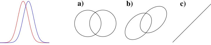
Figure 3: Two Overlapped Gaussian Classes (left), and An Extra Variable (y-axis) Correlated Dif-ferent Amounts (a: no correlation (ρ=0), b: moderate correlation, c: (ρ=1) perfect correlation) with the Unencoded Version of the Regular Input (x-axis).
The extra variable we use is a 1-D value correlated (with correlation ρ) with the unencoded
regular input. For original unencoded input X, the second dimension is drawn from a Gaussian distribution with meanρ×(X−.5)and standard deviationp(1−ρ2). Examples of the distributions
of the unencoded original dimension and the extra variable for various correlations are shown in Figure 3 a,b,and c.
Consider the extreme cases in Figure 3. Atρ=1, the extra variable is exactly an unencoded
version of the regular input. A STD+IN net using this variable as an extra input could ignore the encoded inputs and solve the problem using this variable alone. For few training patterns (relative to the complexity of the encoding), the improvement in performance would be significant. An STD+OUT net using this extra variable as an extra output would have its hidden layer biased towards representations that decode the Gray code, which is also useful to the main classification task. At the other extreme (ρ=0), we expect nets using the extra variable to learn no better than one using just the regular inputs because there is no useful information provided by the uncorrelated extra variable. The interesting case is between the two extremes. We can imagine a situation where as an output, the extra variable helps STD+OUT by guiding it to decode the Gray code. STD+IN though is only helped where the correlation is high enough for the extra variable to be more predictive than the solution the net learns from the regular inputs.
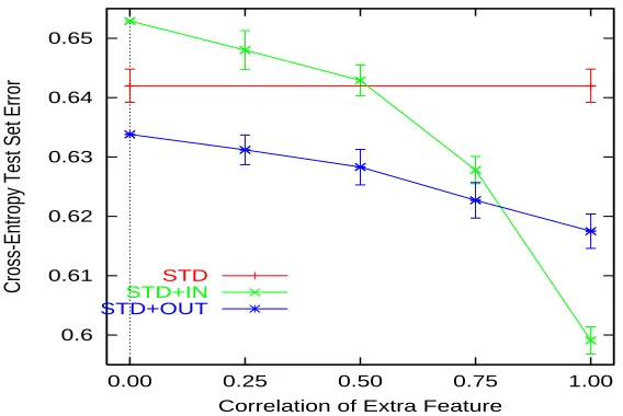
The class output unit uses a sigmoid transfer function and cross-entropy error measure (Bishop, 1995). When used as an extra output, the output unit for the correlated variable uses a linear transfer function and squared error measure. Figure 4 shows the average performance of 50 trials of STD,
STD+IN, and STD+OUT as a function ofρ. As in the previous section, STD+IN is much more
0.6 0.61 0.62 0.63 0.64 0.65
0.00 0.25 0.50 0.75 1.00
Cross-Entropy Test Set Error
Correlation of Extra Feature
STD STD+IN STD+OUT
Figure 4: STD, STD+IN, and STD+OUT vs.ρon the Classification Problem. Error bars are±one
standard error. We could not find the raw data for STD+IN and STD+OUT withρ=0 so
did not construct error bars, but expect that they are comparable to the rest.
2.4 Discussion of Synthetic Problems
The synthetic problems show that the benefit of using a variable as an extra output is different from the benefit of using that variable as an input. As an input, the net has access to the values on the training and test cases, however, as an output, the net is biased to learn a mapping from the other inputs in the training set.
The problems we used to show that some input variables help more as extra outputs are the simplest ones we could devise. One might worry that these effects only happen on simple, or contrived, problems. This is not the case. In Sections 3 and 4 we show similar effects on two real problems. Moreover, these findings explain a result we noted previously, but did not understand, when applying multitask learning to pneumonia risk prediction (Caruana et al., 1996). There, we had the choice of using lab tests that would be unavailable on future patients as extra outputs, or using poor — i.e., noisy — predictions for them as extra inputs. Using the lab tests as extra outputs worked much better, in part because there is no noise in these variables when used as extra outputs because we could use the real values in the training set, not predicted values. If one compares the zero noise points for STD+OUT with the high noise points for STD+IN in the graphs in Section 2.2, it is easy to see why STD+OUT could perform much better.
In order for extra outputs to be more useful than the extra inputs, there must be enough in-formation in the regular inputs to learn the problem. You can’t move all the inputs to the output. Fortunately, in many real world domains there is considerable redundancy in the input variables.
• Select variables for input – call these INPUTS
• Select variables for extra outputs from remaining variables – call these EXTRA OUTPUTS
• Using a regularization method, train an STD+OUT network with #INPUTS input units, a
large number of hidden units, the original outputs plus the EXTRA OUTPUTS as output units
Figure 5: A simple algorithm for combining variable selection and multitask learning.
3. DNA Splice-Junction Problem
DNA contains coded information that is used by cells to construct proteins. In the process of build-ing a message RNA template to use as a scaffold on which to build a protein, large sections of the original DNA coding are ignored. The coded sequences that are used are known as “exons”, while the ignored sequences are known as “introns”. The nature of the boundaries between exons and introns, known as “splice junctions”, is a subject of active research.
The DNA Splice-Junction Problem we use is from the UCI machine learning repository (No-ordewier et al., 1991). For each case in the database there is a sequence of 60 nucleotides. The goal is to predict if the center of the nucleotide sequence codes for an exon-to-intron boundary (EI), an intron-to-exon boundary (IE), or neither. 25% of the cases are EI boundaries, 25% are IE bound-aries, and 50% are neither EI or IE boundaries. For compatibility, we use the nucleotide coding scheme used by Koller and Sahami, which codes each of the 60 nucleotides using 3 bits. This yields 180 boolean attributes that can be used as inputs. Typical performance on this problem is 92-94% accuracy when trained on training sets containing 1000-2000 cases.
3.1 Variable Selection
In real-world problems often there are many irrelevant and redundant variables. Because many learning algorithms have difficulty coping with large numbers of redundant and irrelevant variables, performance often improves when the learning method is given only the subset of variables most useful for the learning task. Variable selection selects from the available variables which ones to use as inputs for learning.
The Koller-Sahami algorithm is a greedy variable selector. The preferred way of using it is backward-elimination. Start with all variables in the set, and remove attributes one-at-a-time, at each step removing the attribute that provides the least information for the class.
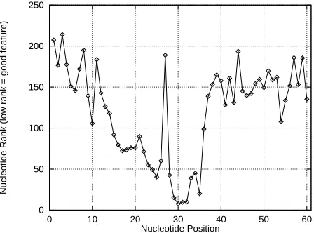
0 50 100 150 200 250
0 10 20 30 40 50 60
Nucleotide Rank (low rank = good feature)
Nucleotide Position
Figure 6: The Order the DNA Features are Selected by Koller-Sahami Variable Selection (More important features are selected first and thus have lower rank).
Figure 6 shows the relative importance of each nucleotide position on the DNA string. The middle of the figure is the position at which we are predicting IE, EI, or Neither. The vertical axis is the sum of the ranks given to the three variables corresponding to each nucleotide, by variable selection. Low ranks suggest that a variable is important and should be used as an input. High ranks indicate variables that contribute little information. The rank sums range from 6 to a maximum of 537 because the rank of each variable ranges from 1 to 180. Note that variable selection for learning was done by looking at each variable individually, not by looking at the nucleotide sums. We show the graph of nucleotide sums because it is much easier to interpret from a biological point of view. Two interesting aspects of this graph are that the most important nucleotides are found near the center of the DNA string, and that nucleotide importance for this task is not symmetric about the center of the DNA string.
3.2 Experiments
We’ve run three experiments with DNA Splice-Junction. In the first, we determine what size net performs best. In the second, we determine if using some variables discarded by variable selection as extra outputs improves performance. In the third experiment, we perform the control of using the inputs as the extra outputs. All our experiments use backprop nets composed of sigmoid units. We train the nets using conjugate gradient and use an independent halt set to determine when to stop training. The performance of the net is then measured on an independent test set not used for training or early stopping. The dataset contains 2000 cases. We randomly split this set into train, halt, and test sets containing 667, 666, and 667 cases, respectively. We repeatedly sample the dataset this way to generate multiple trials.
classification of the net prediction is done by finding which of the three outputs has the highest activation. When boolean attributes are used as extra outputs, we use a non-normalized cross-entropy loss function to train them.
3.2.1 EXPERIMENT1: PERFORMANCE VS. NETSIZE
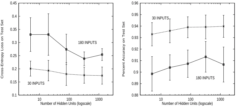
The purpose of this experiment is to determine what net size yields best performance. We tried nets containing 5, 20, 80, 320, and 1280 hidden units. The nets have 3 outputs that code for the main task.
0.1 0.15 0.2 0.25 0.3 0.35 0.4 0.45
10 100 1000
Cross-Entropy Loss on Test Set
Number of Hidden Units (logscale) 180 INPUTS
30 INPUTS
0.88 0.89 0.9 0.91 0.92 0.93 0.94 0.95 0.96
10 100 1000
Percent Accuracy on Test Set
Number of Hidden Units (logscale) 30 INPUTS
180 INPUTS
Figure 7: Cross-Entropy (left) and Accuracy (right) of Different Size Nets With All 180 Inputs and 30 Selected Inputs. Error bars are 95% confidence intervals.
Figure 7 (left) shows the test set cross-entropy error for nets of different sizes trained with all 180 input variables, and trained with the 30 input variables selected by the Koller-Sahami variable selector (these are the same 30 variables Koller and Sahami (1996) selected for this problem). Figure 7 (right) shows the prediction accuracy of the nets. Each point is the average of 12 trials; the vertical bars are 95% confidence intervals.
Better performance is achieved with 80, 320, or 1280 hidden units. Also, performance is sig-nificantly better for nets that use only 30 selected variables as inputs as compared to nets that use all 180 variables as inputs. We conclude from this experiment that the optimal net size is about 320 hidden units, and that training nets with the 30 variables selected with the Koller-Sahami variable selector yields better performance than using all 180 inputs. Because we use the same data to select the optimal network size that is used in later experiments, there may be overfitting. This optimiza-tion is done only for the STD nets, not for the new STD+OUT method, so any overfitting biases the results in favor of the standard method.
3.2.2 EXPERIMENT2: UNUSEDVARIABLES ASEXTRAOUTPUTS
Because the Koller-Sahami variable selector is a greedy algorithm that removes attributes one-at-a-time and is told how many variables to remove, it can be used to order the attributes. We ran Koller-Sahami and had it remove all 180 attributes in the DNA problem. As above, we use the last 30 attributes removed as inputs. Rather than ignore the remaining 150 attributes, we use the next 30 attributes as extra outputs for multitask learning. These are the next attributes of the remaining 150 that the variable selector considers most useful when used as inputs.
The multitask net has 30 inputs, 3 outputs for the main task, and an additional 30 outputs for 30 attributes not selected for use as inputs. The multitask net has 800 hidden units (instead of 320) because it is learning many more tasks. We have not attempted to find the optimal number of hidden units for the multitask net, and suspect it would perform better with more than 800 hidden units.
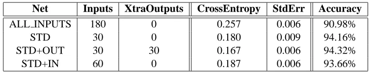
Table 2 shows the cross-entropy and accuracy for four nets. ALL INPUTS has 320 hidden units and uses all 180 inputs. This is a traditional net trained without variable selection. STD also has 320 hidden units, but uses only the 30 variables selected by variable selection as inputs. STD+OUT is the MTL net. It has 800 hidden units and uses the same 30 inputs as STD. STD+OUT, however, also uses the next best 30 attributes as extra outputs. These are attributes ignored by STD. STD+IN has 320 hidden units and uses as inputs both the 30 attributes used by STD as inputs, and the 30 attributes used by STD+OUT as extra outputs. STD+IN uses all attributes used by STD+OUT, but STD+IN uses them as inputs. It has no extra outputs.
Net Inputs XtraOutputs CrossEntropy StdErr Accuracy
ALL INPUTS 180 0 0.257 0.006 90.98%
STD 30 0 0.180 0.009 94.16%
STD+OUT 30 30 0.167 0.006 94.32%
STD+IN 60 0 0.187 0.006 93.66%
Table 2: Cross-Entropy and Accuracy of Different Combinations of Inputs and Outputs. STD+OUT is the MTL Net that Uses Some Variables as Extra Outputs.
ALL INPUTS is clearly the worst performer. Using all 180 attributes as inputs is not the best thing to do. Using only the 30 variables selected by Koller-Sahami as inputs (STD) yields signifi-cantly better performance. STD+OUT, however, performs somewhat better. It is best to use some of the variables not used as inputs as extra outputs instead of ignoring them. STD+IN, which uses all variables used by STD+OUT as inputs, does not perform as well as STD+OUT (nor even as well as STD).2In DNA splice-junction it is better to use some of the variables as extra outputs than as inputs. Moreover, in this domain the Koller-Sahami variable selector with K=0 is an effective way of selecting which variables to use as inputs and which variables are candidates for use as extra outputs.
3.2.3 CONTROL CONDITION: USEDVARIABLES ASEXTRA OUTPUTS
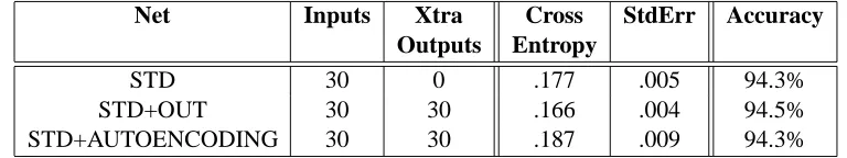
The question arises, is the benefit from using extra outputs, simply due to extra constraints imposed by reconstructing the inputs or due to extracting information from the discarded features? To answer this question, we ran new simulations comparing the STD+OUT network of 30 inputs (and next best 30 inputs as extra outputs) with a network we call STD+AUTOENCODING that has the same 30 inputs and reuses those 30 inputs as its extra outputs (the rest of the variables are discarded).3 The architecture of the STD+OUT and STD+AUTOENCODING networks are identical.
The results are shown below. Note that these experiments were run using a slightly different version of the neural net simulator, and new random selection of training, validation and test sets. All experiments within the table have identical data splits and training conditions, but these are different from those in the table above. Because much of the variance is due to the training/test/valid splits, and we are looking for small effects, it is best to compare results only within a table. The results indicate that the benefit from using extra outputs is not due to simply constraining the network to reconstruct the inputs.
Net Inputs Xtra Cross StdErr Accuracy
Outputs Entropy
STD 30 0 .177 .005 94.3%
STD+OUT 30 30 .166 .004 94.5%
STD+AUTOENCODING 30 30 .187 .009 94.3%
Table 3: Cross-Entropy and Accuracy of Different Combinations of Inputs and Outputs. STD+OUT is the MTL Net that Uses Some (non-Input) Variables as Extra Outputs. STD+AUTOENCODING is the MTL Net that Uses the Inputs as Extra Outputs.
4. Pneumonia Risk-Prediction Problem
The DNA splice-junction problem used in the previous section was downloaded from the UCI Ma-chine Learning Repository. It is a real problem, but has been somewhat pre-processed for maMa-chine learning applications – the data submitted to the UCI Repository was selected to have equal class membership and to have a modest number of input variables, all of which are at least partially relevant to the prediction problem.
The pneumonia problem we experiment with in this section is a real problem that uses real, unsanitized data collected from patients in hospitals in Pennsylvania from 1987-1992. All patients in this database have been diagnosed with pneumonia. The goal is not to diagnose pneumonia, but to predict the risk of a dire outcome for patients with pneumonia. A dire outcome is the occurrence of a serious event such as heart failure, admission to a hospital’s critical care unit, need to use a lung machine, or death. This database was used before in a study comparing the performance of many different machine learning methods (Cooper et al., 1997). In this study, backprop nets were the most effective learning method examined.
The pneumonia dataset contains 192 inputs variables. These variables include patient attributes such as patient age and gender; presence of diabetes, hypertension, asthma, or pregnancy; body
perature and blood pressure; cough type, wheezing, airway blockage; chest X-Ray findings, blood and urine chemistries. The goal is to predict if the patient experiences a dire outcome. Roughly 8% of the patients in the database experience a dire outcome. The performance criterion for this problem is the area under the ROC curve (Provost et al., 1998) for the risk prediction task. The nets are trained with squared error, but early stopping is done using the ROC area measured for the validation set.
4.1 Variable Selection
Variable selection was done using a kernel regression variable selector that does forward selection. The method starts with no variables selected. At each iteration select from the unused variables the one that when added to the previously selected input features yields the best 5-fold cross-validation performance on risk prediction. Eventually, all variables are added to the set, creating an ordering on the variables.
Kernel regression forward selection was used instead of the Koller-Sahami method because many of the variables in the pneumonia problem are continuous and our implementation of Koller-Sahami works only with discrete variables. Forward selection was not done using backprop nets because they are too expensive for forward selection with this many variables, and because their instability makes forward selection more difficult. Kernel regression is far more efficient and is very stable.
We used kernel regression (KR) instead of k-nearest neighbor (KNN) because kernel regression performed somewhat better than k-nearest neighbor on this problem. We suspect similar results would be obtained with either KNN or KR. For kernel regression we used a Gaussian kernel that gives equal weight to the selected features. Each feature was scaled to unit variance prior to doing variable selection to normalize the relative importance of the features in the kernel. The kernel width was selected by leave-one-out cross-validation using all available features as inputs. No attempt was made to re-optimize this kernel width as the number of selected features changed.
Although variable selection was done using kernel regression, neural nets perform significantly better on this problem than any of the k-nearest neighbor methods we tried, so we use backprop nets for our experiments. Preliminary experiments determined that 8-16 hidden units was a good size for backprop nets trained using all 192 input variables, and 64 hidden units was a good size for backprop nets using multitask learning on multiple outputs.
4.2 Experiments
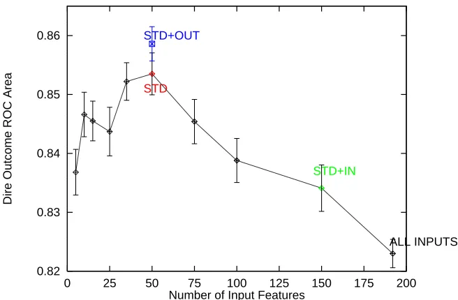
Figure 8 shows the performance of a backprop net trained on the pneumonia problem using different combinations of inputs and extra outputs. The performance measure is ROC Area. Larger ROC Area (up in the figure) represents better performance. An ROC Area of 1.0 indicates perfect prediction. An ROC Area of 0.5 indicates random prediction. The performance in the figure is the ROC Area measured on an independent test set after early stopping is used to halt training of the net. Each point is the average of ten trials. 95% confidence intervals are shown for each point.
as inputs to the backprop net. None of the points on this curve use any of the variables as extra outputs: variables that are not used as inputs are discarded.
Best performance without any extra outputs occurs at the point labeled “STD” when 50 of the 192 variables are used as inputs and the remaining 142 variables are discarded. The performance at this point is 0.03 units larger than the ROC performance when all 192 variables are used as inputs. This is a substantial increase in ROC area and is medically significant. Performance reduces when fewer than 50 or more than 50 variables are used as inputs. Interestingly, performance with only 10 selected variables is better than performance with all 192 variables.
The point labeled “STD+OUT” is the performance obtained if the first 50 variables are used as inputs, and the next 50 variables are used as extra outputs for multitask learning. This performance is better than the performance observed for any combination of input variables alone. This suggests that although the variables ordered 51-100 by the variable selection method are harmful when used as inputs in addition to variables 1-50, there is information in these variables that can beneficially be extracted by multitask learning if these variables are used as extra outputs. For comparison, the point labeled “STD+IN” shows the performance that results from using all variables 1-50 and 51-100 as inputs without any extra outputs. The performance of STD+OUT is considerably better than that of STD+IN, showing that there is a substantial difference between using variables 51-100 as extra outputs instead of as extra inputs. (Although it is not shown in the figure, using variables ordered 1-50 as inputs and the remaining 142 variables as extra outputs does not perform as well as STD+OUT or STD. This suggests that some of the variables do not provide information that is beneficial when used either as inputs or as outputs when variables 1-50 are being used as inputs.)
In summary, the results with a real, unsanitized pneumonia risk problem indicate that there is information in variables that variable selection would discard that multitask learning can exploit if these variables are used as extra outputs. Using some of the variables that would be discarded as extra outputs yields performance that can not be achieved with variable selection alone.
5. Conclusions and Discussion
We have shown two real problems where variable selection improves performance by eliminating input variables, and where performance is further enhanced by using some of the discarded variables as extra outputs. These variables improve performance when used as extra outputs, even though they hurt performance when used as additional inputs. This shows that the benefit of using a variable as an extra output is different from the benefit of using that variable as an input. As an input, the net has access to the variable’s values on the training and test cases. As an output, however, the net is instead biased to learn a mapping from the other input variables to that output. What is learned for this mapping can be useful even when the value of the variable as an additional input is harmful.
0.82 0.83 0.84 0.85 0.86
0 25 50 75 100 125 150 175 200
Dire Outcome ROC Area
Number of Input Features
ALL INPUTS
STD STD+OUT
STD+IN
Figure 8: Results from Experiments on the Pneumonia Risk-Prediction Problem. The error bars are 95% confidence intervals. A paired t-test shows that the difference between STD and STD+OUT is significant at p=0.05.
nets. We present results with backprop nets, however, because preliminary experiments showed that backprop nets outperformed k-nearest neighbor by a significant margin on these two problems.
Recent work also suggests that MTL is effective with Support Vector Machines (Jebara, 2002). Our own experience with SVMs indicates that SVMs benefit from feature selection as much as other learning methods, so we suspect using discarded features as extra outputs may also work with SVMs. When using MTL with SVMs the kernel and the regularization parameters would be shared between the main task and the extra tasks (Cortes and Vapnik, 1995).
One might think that there should be a relationship between causality and which variables should be used as inputs or outputs on a backprop net. We suspect that this is not true for the problems we are studying. Most supervised learning methods are not faithful to the causal arrow. For example, it is common to use supervised learning to diagnose disease by predicting disease (the output) from symptoms (the inputs), despite the fact that the symptoms causally follow from disease. The models we are training learn associations between variables, not causal relations, thus we do not anticipate that causality would help us determine which variables should be used as inputs or outputs, or that one could deduce causal direction from an optimal selection of inputs and outputs.
which it was tested. We currently are working on an algorithm for output selection that would se-lect extra outputs analogous to how inputs are sese-lected by variable sese-lection. We expect improved results with better, principled output selection algorithms.
Selecting the extra outputs after selecting the input variables may also be suboptimal. It is possible that the best network should have fewer input variables than variable selection alone would select, so that some of the variables of marginal utility when used as inputs can be used as extra outputs instead. Similarly, it is possible that some of the inputs variable selection discards would be effective as inputs once one has added other extra outputs to the model. Ultimately, what is needed is an input and output selection method that simultaneously selects which variables should be used as inputs, as extra outputs, and discarded. This is a difficult optimization problem and it is not yet clear how best to approach it.
Still another avenue to explore is whether some variables are best used as both inputs and as outputs. The synthetic problems clearly showed that some variables help when used either as an input, or as an output. We are currently working on several techniques to allow some variables to be used as both inputs and outputs at the same time, and thus reap both benefits.
The experiments with the three synthetic problems clearly demonstrate that the benefit from using variables as inputs or as extra outputs is different. The experiments with the two real problems suggest that similar effects arise on real problems. The performance improvements observed on the real problems, however, are modest. They provide a proof of concept, but are not strong enough for us to recommend using this approach except in domains where small performance improvements are significant. We believe that the benefits will strengthen considerably if we can devise effective procedures for selecting both inputs and extra outputs. We suspect that many real-world problems would benefit from a combination of input and output variable selection and multitask learning if we are able to devise better selection methods.
Acknowledgments
R. Caruana was supported by ARPA grant F33615-93-1-1330, NSF grant BES-9315428, and Agency for Health Care Policy grant HS06468. V. de Sa was supported by a postdoctoral fellowship from the Sloan Foundation and NSF CAREER grant 0133996. We thank the University of Toronto for the Xerion Simulator, D. Koller and M. Sahami for their variable selector, and the editors and anony-mous reviewers for their many helpful suggestions. Preliminary versions of parts of this paper appeared as a NIPS*96 paper and an ICANN 98 paper.
References
Y.S. Abu-Mostafa. Learning from hints in neural networks. Journal of Complexity, 6(2):192–198, 1989.
Shumeet Baluja and Dean A Pomerleau. Using the representation in a neural network’s hidden layer for task-specific focus of attention. In C. Mellish, editor, The International Joint Conference on
Artificial Intelligence 1995 (IJCAI-95), pages 133–139. IJCAI & Morgan Kaufmann, San Mateo,
J. Baxter. Learning internal representations. In Proceedings of the Eleventh Annual Conference on
Computational Learning Theory (COLT-95), 1995.
Suzanna Becker and Geoffrey E. Hinton. Spatial coherence as an internal teacher for a neural network. Technical Report CRG-TR-89-7, University of Toronto, Connectionist Research Group, December 1989.
C. M. Bishop. Neural Networks for Pattern Recognition. Oxford University Press, 1995.
R. Caruana, S. Baluja, and T. Mitchell. Using the future to sort out the present: Rankprop and multitask learning for pneumonia risk prediction. In D.S. Touretzky, M.C. Mozer, and M.E. Hasselmo, editors, Advances in Neural Information Processing Systems 8, pages 959–965. MIT Press, 1996.
Rich Caruana. Learning many related tasks at the same time with backpropagation. In G. Tesauro, D. Touretzky, and T. Leen, editors, Advances in Neural Information Processing Systems 7, pages 657–664. MIT Press, 1995.
Rich Caruana. Applications and algorithms for multitask learning. In ICML-96, pages 87–95, 1996.
Rich Caruana. Multitask learning. Machine Learning, 28:41–75, 1997a.
Rich Caruana. Multitask Learning. PhD thesis, Department of Computer Science, Carnegie Mellon University, 1997b. (available as CMU-CS-97-203).
Rich Caruana and Dayne Freitag. Greedy attribute selection. In ICML-94, pages 28–36, 1994.
G.F. Cooper, C.F. Aliferis, R. Ambrosino, J. Aronis, B.G. Buchanan, R. Caruana, M.J. Fine, C. Gly-mour, G. Gordon, B.H. Hanusa, J.E. Janosky, C. Meek, T. Mitchell, T. Richardson, and P. Spirtes. An evaluation of machine learning methods for predicting pneumonia mortality. Artificial
Intel-ligence in Medicine, 9:107–138, 1997.
C. Cortes and V. Vapnik. Support-vector networks. Machine Learning, 20(3):273–297, 1995.
Virginia R. de Sa. Learning classification with unlabeled data. In J.D. Cowan, G. Tesauro, and J. Alspector, editors, Advances in Neural Information Processing Systems 6, pages 112—119. Morgan Kaufmann, 1994.
Virginia R. de Sa and Dana H. Ballard. Category learning through multimodality sensing. Neural
Computation, 10(5):1097–1117, 1998.
T.G. Dietterich, H. Hild, and G. Bakiri. A comparison of id3 and backpropagation for english text-to-speech mapping. Machine Learning, 18(1):51–80, 1995.
Joumana Ghosn and Yoshua Bengio. Multi-task learning for stock selection. In Michael C. Mozer, Michael I. Jordan, and Thomas Petsche, editors, Advances in Neural Information Processing
Systems 9, pages 946–952. The MIT Press, 1997.
G. John, R. Kohavi, and K. Pfleger. Irrelevant features and the subset selection problem. In
ICML-94, pages 121–129, 1994.
Daphne Koller and M. Sahami. Towards optimal feature selection. In ICML-96, pages 284–292, 1996.
M. Noordewier, G. Towell, and J. Shavlik. Training knowledge-based neural networks to recognize genes in dna sequences. In Richard Lippmann, John E. Moody, and David S. Touretzky, editors,
Advances in Neural Information Processing Systems 3, [NIPS Conference, Denver, Colorado, USA, November 26-29, 1990], pages 530–536. Morgan Kaufmann, 1991.
National Institute of Standards and Technology. Gray code. available electronically at
http://www.nist.gov/dads/HTML/graycode.html.
F. Provost, T. Fawcett, and Ron Kohavi. The case against accuracy estimation for comparing induc-tion algorithms. In ICML-98, pages 445–553, 1998.
D. E. Rumelhart, G. E. Hinton, and R. J. Williams. Learning representations by back-propagating errors. Nature, 323:533—536, 1986.
Patrice Simard, Bernard Victorri, Yann LeCun, and John Denker. Tangent prop — a formalism for specifying selected invariances in an adaptive network. In John E. Moody, Steve J. Hanson, and Richard P. Lippmann, editors, Advances in Neural Information Processing Systems 4, pages 895–903. Morgan Kaufmann Publishers, Inc., 1992.
S.C. Suddarth and A.D.C. Holden. Symbolic-neural systems and the use of hints for developing complex systems. International Journal of Man-Machine Studies, 35(3):291–311, 1991.