A Quasi-Newton Approach to Nonsmooth Convex Optimization Problems in Machine Learning

A Quasi-Newton Approach to Nonsmooth

Convex Optimization Problems in Machine Learning

Jin Yu [email protected]

School of Computer Science The University of Adelaide Adelaide SA 5005, Australia

S.V. N. Vishwanathan [email protected]

Departments of Statistics and Computer Science Purdue University

West Lafayette, IN 47907-2066 USA

Simon G ¨unter GUENTER [email protected]

DV Bern AG

Nussbaumstrasse 21, CH-3000 Bern 22, Switzerland

Nicol N. Schraudolph [email protected]

adaptive tools AG

Canberra ACT 2602, Australia

Editor: Sathiya Keerthi

Abstract

We extend the well-known BFGS quasi-Newton method and its memory-limited variant LBFGS to the optimization of nonsmooth convex objectives. This is done in a rigorous fashion by generalizing three components of BFGS to subdifferentials: the local quadratic model, the identification of a descent direction, and the Wolfe line search conditions. We prove that under some technical conditions, the resulting subBFGS algorithm is globally convergent in objective function value. We apply its memory-limited variant (subLBFGS) to L2-regularized risk minimization with the binary hinge loss. To extend our algorithm to the multiclass and multilabel settings, we develop a new, efficient, exact line search algorithm. We prove its worst-case time complexity bounds, and show that our line search can also be used to extend a recently developed bundle method to the multiclass and multilabel settings. We also apply the direction-finding component of our algorithm to L1-regularized risk minimization with logistic loss. In all these contexts our methods perform comparable to or better than specialized state-of-the-art solvers on a number of publicly available data sets. An open source implementation of our algorithms is freely available.

Keywords: BFGS, variable metric methods, Wolfe conditions, subgradient, risk minimization, hinge loss, multiclass, multilabel, bundle methods, BMRM, OCAS, OWL-QN

1. Introduction

! "(!)

0

acceptable interval

∇_J(wt)⊤pt _c

2∇J(wt)⊤pt c1∇J(wt)⊤pt

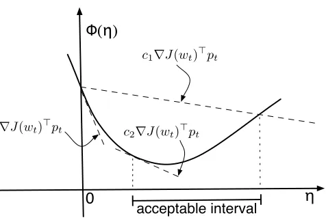
Figure 1: Geometric illustration of the Wolfe conditions (4) and (5).

function J :Rd_→R_{and a current iteratewt ∈}Rd_{, BFGS forms a local quadratic model of J:}

Qt(p) := J(wt) +1₂p⊤Bt−1p+∇J(wt)⊤p, (1)

whereBt≻0 is a positive-definite estimate of the inverse Hessian of J, and∇J denotes the gradient.

Minimizing Qt(p)gives the quasi-Newton direction

p_t:=−B_t∇J(w_t), (2)

which is used for the parameter update:

wt+1=wt+ηtpt. (3)

The step sizeηt >0 is normally determined by a line search obeying the Wolfe (1969) conditions:

J(wt+1) ≤ J(wt) +c1ηt∇J(wt)⊤pt (sufficient decrease) (4)

and ∇J(wt+1)⊤pt ≥ c2∇J(wt)⊤pt (curvature) (5)

with 0<c1<c2<1. Figure 1 illustrates these conditions geometrically. The matrixBt is then

modified via the incremental rank-two update

Bt+1= (I−ρtstyt⊤)Bt(I−ρtytst⊤) +ρtsts⊤t , (6)

wherest :=wt+1−wt andyt :=∇J(wt+1)−∇J(wt)denote the most recent step along the

opti-mization trajectory in parameter and gradient space, respectively, andρt:= (yt⊤st)−1. The BFGS

update (6) enforces the secant equationBt+1yt =st. Given a descent directionpt, the Wolfe

con-ditions ensure that(∀t)s⊤_tyt >0 and henceB0≻0 =⇒ (∀t)Bt≻0.

Limited-memory BFGS (LBFGS, Liu and Nocedal, 1989) is a variant of BFGS designed for

high-dimensional optimization problems where the O(d2)cost of storing and updatingBtwould be

st andyt via a matrix-free approach, reducing the cost to O(md)space and time per iteration, with

m freely chosen.

There have been some attempts to apply (L)BFGS directly to nonsmooth optimization problems, in the hope that they would perform well on nonsmooth functions that are convex and differentiable almost everywhere. Indeed, it has been noted that in cases where BFGS (resp., LBFGS) does not encounter any nonsmooth point, it often converges to the optimum (Lemarechal, 1982; Lewis and Overton, 2008a). However, Lukˇsan and Vlˇcek (1999), Haarala (2004), and Lewis and Overton (2008b) also report catastrophic failures of (L)BFGS on nonsmooth functions. Various fixes can be used to avoid this problem, but only in an ad-hoc manner. Therefore, subgradient-based approaches such as subgradient descent (Nedi´c and Bertsekas, 2000) or bundle methods (Joachims, 2006; Franc and Sonnenburg, 2008; Teo et al., 2010) have gained considerable attention for minimizing nons-mooth objectives.

Although a convex function might not be differentiable everywhere, a subgradient always exists

(Hiriart-Urruty and Lemar´echal, 1993). Letwbe a point where a convex function J is finite. Then

a subgradient is the normal vector of any tangential supporting hyperplane of J atw. Formally,g

is called a subgradient of J atw if and only if (Hiriart-Urruty and Lemar´echal, 1993, Definition

VI.1.2.1)

(∀w′) J(w′) ≥ J(w) + (w′−w)⊤g. (7)

The set of all subgradients at a point is called the subdifferential, and is denoted∂J(w). If this set

is not empty then J is said to be subdifferentiable atw. If it contains exactly one element, that is,

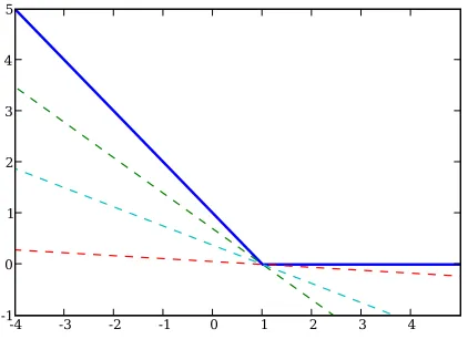
∂J(w) ={∇J(w)}, then J is differentiable atw. Figure 2 provides the geometric interpretation of (7).

The aim of this paper is to develop principled and robust quasi-Newton methods that are amenable to subgradients. This results in subBFGS and its memory-limited variant subLBFGS, two new sub-gradient quasi-Newton methods that are applicable to nonsmooth convex optimization problems. In particular, we apply our algorithms to a variety of machine learning problems, exploiting knowl-edge about the subdifferential of the binary hinge loss and its generalizations to the multiclass and multilabel settings.

In the next section we motivate our work by illustrating the difficulties of LBFGS on nonsmooth functions, and the advantage of incorporating BFGS’ curvature estimate into the parameter update. In Section 3 we develop our optimization algorithms generically, before discussing their application

to L2-regularized risk minimization with the hinge loss in Section 4. We describe a new efficient

algorithm to identify the nonsmooth points of a one-dimensional pointwise maximum of linear functions in Section 5, then use it to develop an exact line search that extends our optimization algorithms to the multiclass and multilabel settings (Section 6). Section 7 compares and contrasts our work with other recent efforts in this area. We report our experimental results on a number of public data sets in Section 8, and conclude with a discussion and outlook in Section 9.

2. Motivation

-4 -3 -2 -1 0 1 2 3 4 -1

0 1 2 3 4 5

Figure 2: Geometric interpretation of subgradients. The dashed lines are tangential to the hinge function (solid blue line); the slopes of these lines are subgradients.

discuss these two aspects of (L)BFGS to motivate our work on developing new quasi-Newton meth-ods that are amenable to subgradients while preserving the fast convergence properties of standard (L)BFGS.

2.1 Problems of (L)BFGS on Nonsmooth Objectives

Smoothness of the objective function is essential for classical (L)BFGS because both the local

quadratic model (1) and the Wolfe conditions (4, 5) require the existence of the gradient∇J at every

point. As pointed out by Hiriart-Urruty and Lemar´echal (1993, Remark VIII.2.1.3), even though nonsmooth convex functions are differentiable everywhere except on a set of Lebesgue measure zero, it is unwise to just use a smooth optimizer on a nonsmooth convex problem under the as-sumption that “it should work almost surely.” Below we illustrate this on both a toy example and real-world machine learning problems.

2.1.1 A TOYEXAMPLE

The following simple example demonstrates the problems faced by BFGS when working with a nonsmooth objective function, and how our subgradient BFGS (subBFGS) method (to be introduced in Section 3) with exact line search overcomes these problems. Consider the task of minimizing

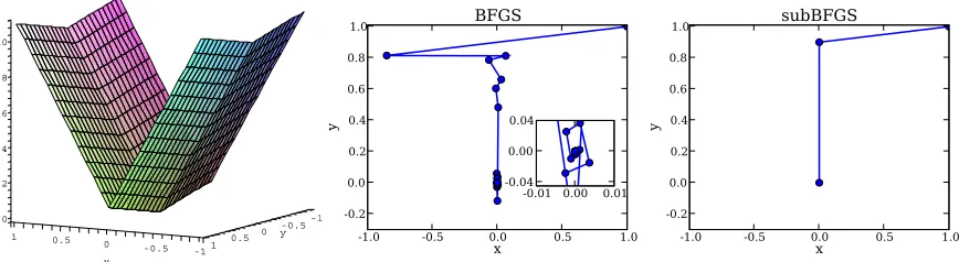
f(x,y) =10|x|+|y| (8)

with respect to x and y. Clearly, f(x,y)is convex but nonsmooth, with the minimum located at(0,0)

(Figure 3, left). It is subdifferentiable whenever x or y is zero:

∂xf(0,·) = [−10,10] and ∂yf(·,0) = [−1,1].

We call such lines of subdifferentiability in parameter space hinges.

-1 -0.5 1

0 2

0 4

6

y 0.5

8 10

x

0 _-0.5 0.5

-11

-1.0 -0.5 0.0 0.5 1.0

x

-0.2 0.0 0.2 0.4 0.6 0.8 1.0

y

BFGS

-0.01 0.00 0.01 -0.04

0.00 0.04

-1.0 -0.5 0.0 0.5 1.0

x

-0.2 0.0 0.2 0.4 0.6 0.8 1.0

y

subBFGS

Figure 3: Left: the nonsmooth convex function (8); optimization trajectory of BFGS with inexact line search (center) and subBFGS (right) on this function.

condition (5), then exponentially decays it until both Wolfe conditions (4, 5) are satisfied.1 The

curvature condition forces BFGS to jump across at least one hinge, thus ensuring that the gradient

displacement vectoryt in (6) is non-zero; this prevents BFGS from diverging. Moreover, with such

an inexact line search BFGS will generally not step on any hinges directly, thus avoiding (in an ad-hoc manner) the problem of non-differentiability. Although this algorithm quickly decreases the

objective from the starting point (1,1), it is then slowed down by heavy oscillations around the

optimum (Figure 3, center), caused by the utter mismatch between BFGS’ quadratic model and the actual function.

A generally sensible strategy is to use an exact line search that finds the optimum along a given descent direction (cf. Section 4.2.1). However, this line optimum will often lie on a hinge (as it does in our toy example), where the function is not differentiable. If an arbitrary subgradient is supplied instead, the BFGS update (6) can produce a search direction which is not a descent direction, causing the next line search to fail. In our toy example, standard BFGS with exact line search consistently

fails after the first step, which takes it to the hinge at x=0.

Unlike standard BFGS, our subBFGS method can handle hinges and thus reap the benefits of an exact line search. As Figure 3 (right) shows, once the first iteration of subBFGS lands it on the

hinge at x=0, its direction-finding routine (Algorithm 2) finds a descent direction for the next step.

In fact, on this simple example Algorithm 2 yields a vector with zero x component, which takes

subBFGS straight to the optimum at the second step.2

2.1.2 TYPICALNONSMOOTHOPTIMIZATIONPROBLEMS INMACHINELEARNING

The problems faced by smooth quasi-Newton methods on nonsmooth objectives are not only en-countered in cleverly constructed toy examples, but also in real-world applications. To show this,

we apply LBFGS to L2-regularized risk minimization problems (30) with binary hinge loss (31), a

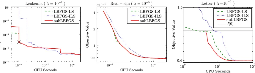
typical nonsmooth optimization problem encountered in machine learning. For this particular ob-jective function, an exact line search is cheap and easy to compute (see Section 4.2.1 for details). Figure 4 (left & center) shows the behavior of LBFGS with this exact line search (LBFGS-LS)

100 101 102

CPU Seconds

0.6 1.5

Objective Value

Letter ( =10!6

)

LBFGS-LS LBFGS-ILS subLBFGS J(0)

Figure 4: Performance of subLBFGS (solid) and standard LBFGS with exact (dashed) and inexact

(dotted) line search methods on sample L2-regularized risk minimization problems with

the binary (left and center) and multiclass hinge losses (right). LBFGS with exact line

search (dashed) fails after 3 iterations (marked as×) on the Leukemia data set (left).

on two data sets, namely Leukemia and Real-sim.3 It can be seen that LBFGS-LS converges on

Real-sim but diverges on the Leukemia data set. This is because using an exact line search on a nonsmooth objective function increases the chance of landing on nonsmooth points, a situation that standard BFGS (resp., LBFGS) is not designed to deal with. To prevent (L)BFGS’ sudden break-down, a scheme that actively avoids nonsmooth points must be used. One such possibility is to use an inexact line search that obeys the Wolfe conditions. Here we used an efficient inexact line

search that uses a caching scheme specifically designed for L2-regularized hinge loss (cf. end of

Section 4.2). This implementation of LBFGS (LBFGS-ILS) converges on both data sets shown here but may fail on others. It is also slower, due to the inexactness of its line search.

For the multiclass hinge loss (42) we encounter another problem: if we follow the usual practice

of initializingw=0_{, which happens to be a non-differentiable point, then LBFGS stalls. One way}

to get around this is to force LBFGS to take a unit step along its search direction to escape this

nonsmooth point. However, as can be seen on the Letter data set3in Figure 4 (right), such an ad-hoc

fix increases the value of the objective above J(0_{)(solid horizontal line), and it takes several CPU}

seconds for the optimizers to recover from this. In all cases shown in Figure 4, our subgradient LBFGS (subLBFGS) method (as will be introduced later) performs comparable to or better than the best implementation of LBFGS.

2.2 Advantage of Incorporating BFGS’ Curvature Estimate

In machine learning one often encounters L2-regularized risk minimization problems (30) with

var-ious hinge losses (31, 42, 55). Since the Hessian of those objective functions at differentiable points

equals λI (where λ is the regularization constant), one might be tempted to argue that for such

problems, BFGS’ approximation Bt to the inverse Hessian should be simply set to λ−1I. This

would reduce the quasi-Newton directionpt =−Btgt, gt ∈∂J(wt)to simply a scaled subgradient

direction.

To check if doing so is beneficial, we compared the performance of our subLBFGS method with two implementations of subgradient descent: a vanilla gradient descent method (denoted GD) that

100 ₁₀1 ₁₀2 ₁₀3 CPU Seconds

1.2 2 3 4

Objective Value

CCAT ( =10!6

)

GD subGD subLBFGS

x10"1

101 ₁₀2 ₁₀3

CPU Seconds 0.3

1.0

Objective Value

INEX ( =10!6

)

GD subGD subLBFGS

101 ₁₀2 ₁₀3 ₁₀4

CPU Seconds 0.4

1.0

Objective Value

TMC2007 ( =10!5

)

GD subGD subLBFGS

Figure 5: Performance of subLBFGS, GD, and subGD on sample L2-regularized risk minimization

problems with binary (left), multiclass (center), and multilabel (right) hinge losses.

0.0 0.5 1.0 1.5 2.0 2.5 3.0 3.5 4.0 0.6

0.8 1.0 1.2 1.4 1.6 1.8 2.0

BFGS Quadratic Model Piecewise Linear Function

0.0 0.5 1.0 1.5 2.0 2.5 3.0 3.5 4.0

-1.5 -1.0 -0.5 0.0 0.5 1.0 1.5

Gradient of BFGS Model Piecewise Constant Gradient

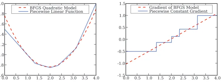
Figure 6: BFGS’ quadratic approximation to a piecewise linear function (left), and its estimate of the gradient of this function (right).

uses a random subgradient for its parameter update, and an improved subgradient descent method (denoted subGD) whose parameter is updated in the direction produced by our direction-finding

routine (Algorithm 2) with Bt =I. All algorithms used exact line search, except that GD took

a unit step for the first update in order to avoid the nonsmooth pointw0=0 (cf. the discussion

in Section 2.1). As can be seen in Figure 5, on all sample L2-regularized hinge loss minimization

problems, subLBFGS (solid) converges significantly faster than GD (dotted) and subGD (dashed).

This indicates that BFGS’Bt matrix is able to model the objective function, including its hinges,

better than simply settingBt to a scaled identity matrix.

We believe that BFGS’ curvature update (6) plays an important role in the performance of

subLBFGS seen in Figure 5. Recall that (6) satisfies the secant conditionBt+1yt=st, wherestand

yt are displacement vectors in parameter and gradient space, respectively. The secant condition in

we have

Bt+1=

(w+p)−w

∇J(w+p)−∇J(w). (9)

Although the original motivation behind the secant condition was to approximate the inverse Hes-sian, the finite differencing scheme (9) allows BFGS to model the global curvature (i.e., overall shape) of the objective function from first-order information. For instance, Figure 6 (left) shows

that the BFGS quadratic model4 _{(1) fits a piecewise linear function quite well despite the fact that}

the actual Hessian in this case is zero almost everywhere, and infinite (in the limit) at nonsmooth points. Figure 6 (right) reveals that BFGS captures the global trend of the gradient rather than its in-finitesimal variation, that is, the Hessian. This is beneficial for nonsmooth problems, where Hessian does not fully represent the overall curvature of the objective function.

3. Subgradient BFGS Method

We modify the standard BFGS algorithm to derive our new algorithm (subBFGS, Algorithm 1) for nonsmooth convex optimization, and its memory-limited variant (subLBFGS). Our modifications can be grouped into three areas, which we elaborate on in turn: generalizing the local quadratic model, finding a descent direction, and finding a step size that obeys a subgradient reformulation of the Wolfe conditions. We then show that our algorithm’s estimate of the inverse Hessian has a bounded spectrum, which allows us to prove its convergence.

Algorithm 1 Subgradient BFGS (subBFGS)

1: Initialize: t :=0,w0=0,B0=I

2: Set: direction-finding toleranceε≥0, iteration limit kmax>0,

lower bound h>0 on s⊤tyt

yt⊤yt (cf. discussion in Section 3.4)

3: Compute subgradientg0∈∂J(w0)

4: while not converged do

5: pt=descentDirection(gt,ε,kmax) (Algorithm 2)

6: ifpt=failure then

7: Returnwt

8: end if

9: Findηt that obeys (23) and (24) (e.g., Algorithm 3 or 5)

10: st=ηtpt

11: wt+1=wt+st

12: Choose subgradientgt+1∈∂J(wt+1):st⊤(gt+1−gt)>0

13: yt:=gt+1−gt

14: st:=st+max

0,h−st⊤yt y⊤tyt

yt (ensure s

⊤

tyt yt⊤yt ≥h)

15: UpdateBt+1via (6)

16: t :=t+1

17: end while

-4 -3 -2 -1 0 1 2 3 4 -1

0 1 2 3 4 5

-4 -3 -2 -1 0 1 2 3 4

-1 0 1 2 3 4 5

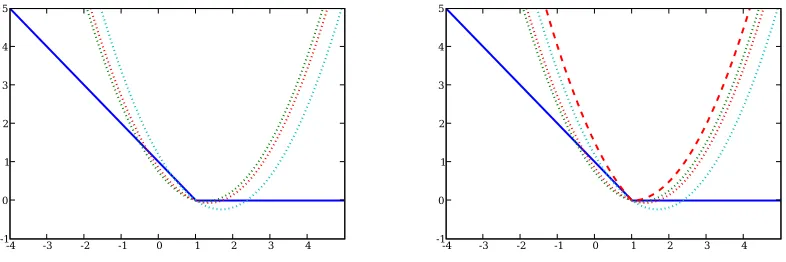
Figure 7: Left: selecting arbitrary subgradients yields many possible quadratic models (dotted lines) for the objective (solid blue line) at a subdifferentiable point. The models were

built by keepingBt fixed, but selecting random subgradients. Right: the tightest

pseudo-quadratic fit (10) (bold red dashes); note that it is not a pseudo-quadratic.

3.1 Generalizing the Local Quadratic Model

Recall that BFGS assumes that the objective function J is differentiable everywhere so that at the

current iteratewt it can construct a local quadratic model (1) of J(wt). For a nonsmooth objective

function, such a model becomes ambiguous at non-differentiable points (Figure 7, left). To resolve

the ambiguity, we could simply replace the gradient ∇J(wt) in (1) with an arbitrary subgradient

gt∈∂J(wt). However, as will be discussed later, the resulting quasi-Newton directionpt:=−Btgt

is not necessarily a descent direction. To address this fundamental modeling problem, we first generalize the local quadratic model (1) as follows:

Qt(p) := J(wt) +Mt(p), where

Mt(p) := ₂1p⊤Bt−1p + sup g∈∂J(wt)

g⊤p. (10)

Note that where J is differentiable, (10) reduces to the familiar BFGS quadratic model (1). At non-differentiable points, however, the model is no longer quadratic, as the supremum may be attained

at different elements of∂J(wt)for different directionsp. Instead it can be viewed as the tightest

pseudo-quadratic fit to J at wt (Figure 7, right). Although the local model (10) of subBFGS is

nonsmooth, it only incorporates non-differential points present at the current location; all others are smoothly approximated by the quasi-Newton mechanism.

Having constructed the model (10), we can minimize Qt(p), or equivalently Mt(p):

min p∈Rd

1 2p

⊤_B−1

t p + sup

g∈∂J(wt)

g⊤p

!

(11)

as the solution to the following problem (Hiriart-Urruty and Lemar´echal, 1993, Chapter VIII):

min p∈Rd J

′_(w

t,p) s.t. |||p||| ≤1, (12)

where

J′(wt, p):=lim η↓0

J(wt+ηp)−J(wt)

η

is the directional derivative of J atwt in direction p, and ||| · |||is a norm defined onRd. In other

words, the normalized steepest descent direction is the direction of bounded norm along which the maximum rate of decrease in the objective function value is achieved. Using the property:

J′(w_t,p) =sup_g∈∂J(wt)g⊤p(Bertsekas, 1999, Proposition B.24.b), we can rewrite (12) as:

min p∈Rd sup

g∈∂J(wt)

g⊤p s.t. |||p||| ≤1. (13)

If the matrixBt≻0 as in (11) is used to define the norm||| · |||as

|||p|||2:=p⊤B_t−1p, (14) then the solution to (13) points to the same direction as that obtained by minimizing our pseudo-quadratic model (11). To see this, we write the Lagrangian of the constrained minimization problem (13):

L(p,α) :=αp⊤B_t−1p −α + sup g∈∂J(wt)

g⊤p

= 1₂p⊤(2αB_t−1)p −α + sup g∈∂J(wt)

g⊤p, (15)

whereα>0 is a Lagrangian multiplier. It is easy to see from (15) that minimizing the Lagrangian

function L with respect topis equivalent to solving (11) withB_t−1scaled by a scalar 2α, implying

that the steepest descent direction obtained by solving (13) with the weighted norm (14) only differs in length from the search direction obtained by solving (11). Therefore, our search direction is essentially an unnomalized steepest descent direction with respect to the weighted norm (14).

Ideally, we would like to solve (11) to obtain the best search direction. This is generally

in-tractable due to the presence a supremum over the entire subdifferential set∂J(wt). In many

ma-chine learning problems, however,∂J(wt)has some special structure that simplifies the calculation

of that supremum. In particular, the subdifferential of all the problems considered in this paper is a convex and compact polyhedron characterised as the convex hull of its extreme points. This

dra-matically reduces the cost of calculating sup_g∈∂J(wt)g⊤psince the supremum can only be attained

at an extreme point of the polyhedral set∂J(wt)(Bertsekas, 1999, Proposition B.21c). In what

fol-lows, we develop an iterative procedure that is guaranteed to find a quasi-Newton descent direction,

assuming an oracle that supplies arg sup_g∈∂J(wt)g⊤pfor a given directionp∈Rd_{. Efficient oracles}

for this purpose can be derived for many machine learning settings; we provides such oracles for

L2-regularized risk minimization with the binary hinge loss (Section 4.1), multiclass and multilabel

Algorithm 2 pt=descentDirection(g(1),ε,kmax) 1: input (sub)gradientg(1)_∈∂J(w

t), toleranceε≥0, iteration limit kmax>0,

and an oracle to calculate arg sup_g∈∂J(w)g⊤pfor any givenwandp

2: output descent directionpt

3: Initialize: i=1, g¯(1)_=g(1)_,p(1)_=−B tg(1)

4: g(2)=arg sup_g∈∂J(wt)g⊤p(1)

5: ε(1):=p(1)⊤_g(2)_−p(1)⊤_g¯(1)

6: while(g(i+1)⊤_p(i)_{>0 orε}(i)_>ε)andε(i)_{>0 and i<k}

maxdo 7: µ∗:=minh1, (g¯(i)−g(i+1))⊤Btg¯(i)

(g¯(i)_−g(i+1)₎⊤_Bt(g¯(i)_−g(i+1)₎

i

; see (97)

8: g¯(i+1)= (1−µ∗)g¯(i)+µ∗g(i+1)

9: p(i+1)= (1−µ∗)p(i)_−µ∗_B

tg(i+1); see (76)

10: g(i+2)=arg sup_g∈∂J(wt)g⊤p(i+1)

11: ε(i+1):=minj≤(i+1)

p(j)⊤g(j+1)−1

2(p(

j)⊤_g¯(j)_+p(i+1)⊤_g¯(i+1)₎

12: i :=i+1

13: end while

14: pt =argminj≤iMt(p(j))

15: if sup_g∈∂J(wt)g⊤pt≥0 then

16: return failure;

17: else

18: returnpt.

19: end if

3.2 Finding a Descent Direction

A direction pt is a descent direction if and only if g⊤pt <0 ∀g ∈∂J(wt) (Hiriart-Urruty and

Lemar´echal, 1993, Theorem VIII.1.1.2), or equivalently

sup g∈∂J(wt)

g⊤pt < 0. (16)

For a smooth convex function, the quasi-Newton direction (2) is always a descent direction because

∇J(wt)⊤pt =−∇J(wt)⊤Bt∇J(wt) < 0

holds due to the positivity ofBt.

For nonsmooth functions, however, the quasi-Newton direction pt :=−Btgt for a givengt ∈

∂J(wt)may not fulfill the descent condition (16), making it impossible to find a step sizeη>0

that obeys the Wolfe conditions (4, 5), thus causing a failure of the line search. We now present an iterative approach to finding a quasi-Newton descent direction.

Our goal is to minimize the pseudo-quadratic model (10), or equivalently minimize Mt(p).

Inspired by bundle methods (Teo et al., 2010), we achieve this by minimizing convex lower bounds

of Mt(p)that are designed to progressively approach Mt(p)over iterations. At iteration i we build

the following convex lower bound on Mt(p):

Mt(i)(p) := 1₂p⊤Bt−1p+sup j≤i

where i,j∈N_andg(j)_∈∂J(w

t) ∀j≤i. Given a p(i)∈Rd the lower bound (17) is successively

tightened by computing

g(i+1):= arg sup g∈∂J(wt)

g⊤p(i), (18)

such that M_t(i)(p)≤M_t(i+1)(p)≤Mt(p)∀p∈Rd. Here we setg(1)∈∂J(wt)arbitrarily, and assume

that (18) is provided by an oracle (e.g., as described in Section 4.1). To solve min_p∈RdM(_ti)(p), we

rewrite it as a constrained optimization problem:

min p,ξ

1 2p

⊤_B−1

t p+ξ

s.t. g(j)⊤p≤ξ ∀j≤i. (19)

This problem can be solved exactly via quadratic programming, but doing so may incur substantial computational expense. Instead we adopt an alternative approach (Algorithm 2) which does not

solve (19) to optimality. The key idea is to write the proposed descent direction at iteration i+1

as a convex combination ofp(i)_and−B

tg(i+1) (Line 9 of Algorithm 2); and as will be shown in

Appendix B, the returned search direction takes the form

pt=−Btg¯t,

where ¯gt is a subgradient in∂J(wt) that allowspt to satisfy the descent condition (16). The

opti-mal convex combination coefficient µ∗can be computed exactly (Line 7 of Algorithm 2) using an

argument based on maximizing the dual objective of Mt(p); see Appendix A for details.

The weak duality theorem (Hiriart-Urruty and Lemar´echal, 1993, Theorem XII.2.1.5) states that

the optimal primal value is no less than any dual value, that is, if Dt(α)is the dual of Mt(p), then

min_p∈RdM_t(p)≥D_t(α)holds for all feasible dual solutionsα. Therefore, by iteratively increasing

the value of the dual objective we close the gap to optimality in the primal. Based on this argument, we use the following upper bound on the duality gap as our measure of progress:

ε(i)_:=min j≤i

h

p(j)⊤g(j+1)−1₂(p(j)⊤g¯(j)+p(i)⊤g¯(i))i≥ min

p∈RdMt(p)−Dt(α

∗_{), (20)}

where ¯g(i) _{is an aggregated subgradient (Line 8 of Algorithm 2) which lies in the convex hull of}

g(j)_∈∂J(w

t)∀j≤i, andα∗is the optimal dual solution; Equations 77–79 in Appendix A provide

intermediate steps that lead to the inequality in (20). Theorem 7 (Appendix B) shows thatε(i) is

monotonically decreasing, leading us to a practical stopping criterion (Line 6 of Algorithm 2) for our direction-finding procedure.

A detailed derivation of Algorithm 2 is given in Appendix A, where we also prove that at a

non-optimal iterate a direction-finding toleranceε≥0 exists such that the search direction produced by

Algorithm 2 is a descent direction; in Appendix B we prove that Algorithm 2 converges to a solution

with precisionε in O(1/ε)iterations. Our proofs are based on the assumption that the spectrum

(eigenvalues) of BFGS’ approximationBt to the inverse Hessian is bounded from above and below.

3.3 Subgradient Line Search

Given the current iteratewt and a search directionpt, the task of a line search is to find a step size

η>0 which reduces the objective function value along the linewt+ηpt:

minimize Φ(η) :=J(wt+ηpt). (21)

Using the chain rule, we can write

∂Φ(η) :={g⊤p_t:g∈∂J(w_t+ηp_t)}. (22)

Exact line search finds the optimal step sizeη∗by minimizingΦ(η), such that 0∈∂Φ(η∗_{); inexact}

line searches solve (21) approximately while enforcing conditions designed to ensure convergence. The Wolfe conditions (4) and (5), for instance, achieve this by guaranteeing a sufficient decrease in the value of the objective and excluding pathologically small step sizes, respectively (Wolfe, 1969; Nocedal and Wright, 1999). The original Wolfe conditions, however, require the objective function to be smooth; to extend them to nonsmooth convex problems, we propose the following subgradient reformulation:

J(w_t+1) ≤ J(w_t) + c1ηt sup g∈∂J(wt)

g⊤p_t (sufficient decrease) (23)

and sup

g′_{∈∂J(wt+1)}

g′⊤p_t ≥ c2 sup

g∈∂J(wt)

g⊤p_t, (curvature) (24)

where 0<c1<c2<1. Figure 8 illustrates how these conditions enforce acceptance of non-trivial

step sizes that decrease the objective function value. In Appendix C we formally show that for any given descent direction we can always find a positive step size that satisfies (23) and (24). Moreover, Appendix D shows that the sufficient decrease condition (23) provides a necessary condition for the global convergence of subBFGS.

Employing an exact line search is a common strategy to speed up convergence, but it drastically increases the probability of landing on a non-differentiable point (as in Figure 4, left). In order to leverage the fast convergence provided by an exact line search, one must therefore use an optimizer that can handle subgradients, like our subBFGS.

A natural question to ask is whether the optimal step size η∗obtained by an exact line search

satisfies the reformulated Wolfe conditions (resp., the standard Wolfe conditions when J is smooth).

The answer is no: depending on the choice of c1,η∗may violate the sufficient decrease condition

(23). For the function shown in Figure 8, for instance, we can increase the value of c1 such that

the acceptable interval for the step size excludesη∗. In practice one can set c1to a small value, for

example, 10−4, to prevent this from happening.

The curvature condition (24), on the other hand, is always satisfied by η∗, as long as pt is a

descent direction (16):

sup g′_∈J(wt+η∗_pt)

g′⊤pt = sup

g∈∂Φ(η∗₎

g ≥ 0 > sup g∈∂J(wt)

g⊤pt

! "(!)

0

acceptable interval c1 sup

g∈∂J(wt)

g⊤pt

c2 sup g∈∂J(wt)

g⊤pt inf

g∈∂J(wt)

g⊤pt

sup g∈∂J(wt)

g⊤pt

Figure 8: Geometric illustration of the subgradient Wolfe conditions (23) and (24). Solid disks are subdifferentiable points; the slopes of dashed lines are indicated.

3.4 Bounded Spectrum of SubBFGS’ Inverse Hessian Estimate

Recall from Section 1 that to ensure positivity of BFGS’ estimate Bt of the inverse Hessian, we

must have(∀t)s⊤_t yt>0. Extending this condition to nonsmooth functions, we require

(wt+1−wt)⊤(gt+1−gt)>0, where gt+1∈∂J(wt+1) and gt∈∂J(wt). (25)

If J is strongly convex,5andwt+16=wt, then (25) holds for any choice ofgt+1andgt.6For general

convex functions,gt+1need to be chosen (Line 12 of Algorithm 1) to satisfy (25). The existence of

such a subgradient is guaranteed by the convexity of the objective function. To see this, we first use

the fact thatηtpt =wt+1−wt andηt >0 to rewrite (25) as

p⊤_t gt+1>pt⊤gt, where gt+1∈∂J(wt+1) and gt∈∂J(wt). (26)

It follows from (22) that both sides of inequality (26) are subgradients ofΦ(η)atηt and 0,

respec-tively. The monotonic property of∂Φ(η)given in Theorem 1 (below) ensures thatp⊤_t gt+1is no less

thanp⊤_t gt for any choice ofgt+1andgt, that is,

inf g∈∂J(wt+1)p

⊤

t g ≥ sup

g∈∂J(wt)

p⊤_t g. (27)

This means that the only case where inequality (26) is violated is when both terms of (27) are equal, and

gt+1= arg inf

g∈∂J(wt+1)

g⊤pt and gt= arg sup

g∈∂J(wt)

g⊤pt,

that is, in this casep⊤_t gt+1=p⊤t gt. To avoid this, we simply need to setgt+1to a different

subgra-dient in∂J(wt+1).

5. If J is strongly convex, then(g2−g1)⊤(w2−w1)≥ckw2−w1k2, with c>0,gi∈∂J(wi),i=1,2.

Theorem 1 (Hiriart-Urruty and Lemar´echal, 1993, Theorem I.4.2.1)

LetΦbe a one-dimensional convex function on its domain, then∂Φ(η) is increasing in the sense that g1≤g2 whenever g1∈∂Φ(η1), g2∈∂Φ(η2),andη1<η2.

Our convergence analysis for the direction-finding procedure (Algorithm 2) as well as the global

convergence proof of subBFGS in Appendix D require the spectrum ofBtto be bounded from above

and below by a positive scalar:

∃(h,H : 0<h≤H<∞):(∀t)hBt H. (28)

From a theoretical point of view it is difficult to guarantee (28) (Nocedal and Wright, 1999, page

212), but based on the fact thatBt is an approximation to the inverse HessianHt−1, it is reasonable

to expect (28) to be true if

(∀t)1/HHt 1/h.

Since BFGS “senses” the Hessian via (6) only through the parameter and gradient displacementsst

andyt, we can translate the bounds on the spectrum ofHt into conditions that only involvest and

yt:

(∀t) s ⊤

t yt s⊤_t st

≥ 1

H and

y_t⊤yt

s⊤_t yt

≤1

h, with 0<h≤H<∞. (29)

This technique is used in Nocedal and Wright (1999, Theorem 8.5). If J is strongly convex5 and

st6=0, then there exists an H such that the left inequality in (29) holds. On general convex functions,

one can skip BFGS’ curvature update if (s⊤_t yt/s⊤t st) falls below a threshold. To establish the

second inequality, we add a fraction ofyttost at Line 14 of Algorithm 1 (though this modification

is never actually invoked in our experiments of Section 8, where we set h=10−8).

3.5 Limited-Memory Subgradient BFGS

It is straightforward to implement an LBFGS variant of our subBFGS algorithm: we simply modify

Algorithms 1 and 2 to compute all products between Bt and a vector by means of the standard

LBFGS matrix-free scheme (Nocedal and Wright, 1999, Algorithm 9.1). We call the resulting algorithm subLBFGS.

3.6 Convergence of Subgradient (L)BFGS

In Section 3.4 we have shown that the spectrum of subBFGS’ inverse Hessian estimate is bounded. From this and other technical assumptions, we prove in Appendix D that subBFGS is globally

con-vergent in objective function value, that is, J(w)→infwJ(w). Moreover, in Appendix E we show

that subBFGS converges for all counterexamples we could find in the literature used to illustrate the non-convergence of existing optimization methods on nonsmooth problems.

0 200 400 600 800 1000 1200 1400 1600 Iterations

10-10 10-9 10-8 10-7 10-6 10-5 10-4 10-3 10-2 10-1 100

J(

wt

)

J

!

CCAT ("

=10#6

)

0 500 1000 1500 2000 2500 3000 3500 4000 Iterations

10-9 10-8 10-7 10-6 10-5 10-4 10-3 10-2 10-1 100

J(

wt

)

J

!

INEX ("

=10#6

)

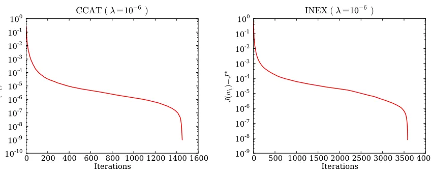
Figure 9: Convergence of subLBFGS in objective function value on sample L2-regularized risk

minimization problems with binary (left) and multiclass (right) hinge losses.

in Figure 9, where we plot (on a log scale) the excess objective function value J(wt)over its

“opti-mum” J∗7against the iteration number in two typical runs. The same kind of convergence behavior

was observed by Lewis and Overton (2008a, Figure 5.7), who applied the classical BFGS algorithm with a specially designed line search to nonsmooth functions. They caution that the apparent super-linear convergence may be an artifact caused by the inaccuracy of the estimated optimal value of the objective.

4. SubBFGS for L2-Regularized Binary Hinge Loss

Many machine learning algorithms can be viewed as minimizing the L2-regularized risk

J(w) := λ

2kwk

2₊ 1

n

n

∑

l(xi,zi,w), (30)

whereλ>0 is a regularization constant,xi∈

X

Z

cor-responding labels, and the loss l is a non-negative convex function ofwwhich measures the

dis-crepancy between zi and the predictions arising from usingw. A loss function commonly used for

binary classification is the binary hinge loss

l(x,z,w) := max(0,1−zw⊤x), (31)

where z∈ {±1}. L2-regularized risk minimization with the binary hinge loss is a convex but

nons-mooth optimization problem; in this section we show how subBFGS (Algorithm 1) can be applied to this problem.

Let

E

M

W

respectively:

E

M

W

Differentiating (30) after plugging in (31) then yields

∂J(w) = λw−1

n

n

∑

βizixi = w¯ −

1

n

∑

i∈M

βizixi, (32)

where w¯ :=λw−1

n_i

∑

zixi and βi:=

 



1 if i∈

E

[0,1] if i∈

M

0 if i∈

W

4.1 Efficient Oracle for the Direction-Finding Method

Recall that subBFGS requires an oracle that provides arg sup_g∈∂J(wt)g⊤pfor a given directionp.

For L2-regularized risk minimization with the binary hinge loss we can implement such an oracle

at a computational cost of O(d|

M

M

current margin points, which is normally much less than n. Towards this end, we use (32) to obtain

sup g∈∂J(wt)

g⊤p = sup

βi,i∈M_t

¯

wt−

1

n_i∈

∑

t βizixi

!⊤

p

= w¯_t⊤p−1

n_i∈

∑

t inf

βi∈[0,1](βizix

⊤

i p). (33)

Since for a givenpthe first term of the right-hand side of (33) is a constant, the supremum is attained

when we setβi∀i∈

M

βi:=

(

0 if zix⊤i pt ≥0,

1 if zix⊤i pt <0.

4.2 Implementing the Line Search

The one-dimensional convex functionΦ(η):=J(w+ηp)(Figure 10, left) obtained by restricting

(30) to a line can be evaluated efficiently. To see this, rewrite (30) as

J(w) := λ

2kwk

2₊ 1

n1

⊤_{max(0,1−z·Xw), (34)}

where0_and1_{are column vectors of zeros and ones, respectively,·denotes the Hadamard}

(component-wise) product, and z ∈Rn _{collects correct labels corresponding to each row of data in X :=}

[x1,x2,· · ·,xn]⊤∈Rn×d. Given a search directionpat a pointw, (34) allows us to write

Φ(η) = λ

2kwk

2_+ληw⊤_p+ λη2

2 kpk

2₊ 1

n1

´

)

´

(

©

´

S

ub

g

ra

d

ie

nt

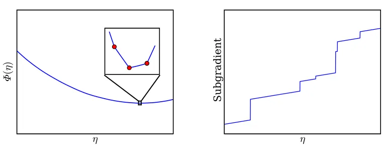
Figure 10: Left: Piecewise quadratic convex functionΦof step sizeη; solid disks in the zoomed

inset are subdifferentiable points. Right: The subgradient ofΦ(η)increases

monotoni-cally withη, and jumps discontinuously at subdifferentiable points.

wheref:=z·Xwand∆f:=z·Xp. Differentiating (35) with respect toηgives the subdifferential

ofΦ:

∂Φ(η) =λw⊤p+ηλkpk2₋1

nδ(η)

⊤_{∆f, (36)}

whereδ:R_→Rn_{outputs a column vector[}δ₁₍η_),δ₂₍η_{),· · ·,}δ_n(η_)]⊤_with

δi(η):=

 



1 if fi+η∆fi <1,

[0,1] if fi+η∆fi =1,

0 if fi+η∆fi >1.

(37)

We cachef and∆f, expending O(nd)computational effort and using O(n) storage. We also

cache the scalars λ₂kwk2_,λ_w⊤_{p, and} λ

2kpk2, each of which requires O(d)work. The evaluation of

1_−(f+η∆_f),δ(η_{), and the inner products in the final terms of (35) and (36) all take O(n)effort.}

Given the cached terms, all other terms in (35) can be computed in constant time, thus reducing the

cost of evaluatingΦ(η)(resp., its subgradient) to O(n). Furthermore, from (37) we see thatΦ(η)is

differentiable everywhere except at

ηi:= (1−fi)/∆fi with ∆fi6=0, (38)

where it becomes subdifferentiable. At these points an element of the indicator vector (37) changes from 0 to 1 or vice versa (causing the subgradient to jump, as shown in Figure 10, right); otherwise

δ(η)remains constant. Using this property ofδ(η), we can update the last term of (36) in constant

!! ! "(!)

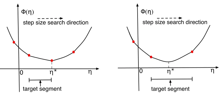
0

target segment

step size search direction

!! !

"(!)

0

target segment step size search direction

Figure 11: Nonsmooth convex functionΦ of step sizeη. Solid disks are subdifferentiable points;

the optimal stepη∗ either falls on such a point (left), or lies between two such points

(right).

4.2.1 EXACTLINE SEARCH

Given a directionp, exact line search finds the optimal step sizeη∗:=argmin_η≥0Φ(η)that satisfies

0∈∂Φ(η∗), or equivalently

inf∂Φ(η∗)≤0≤sup∂Φ(η∗).

By Theorem 1, sup∂Φ(η)is monotonically increasing withη. Based on this property, our algorithm

first builds a list of all possible subdifferentiable points andη=0, sorted by non-descending value

of η (Lines 4–5 of Algorithm 3). Then, it starts with η=0, and walks through the sorted list

until it locates the “target segment”, an interval [ηa,ηb]between two subdifferential points with

sup∂Φ(ηa)≤0 and sup∂Φ(ηb)≥0. We now know that the optimal step size either coincides with

ηb(Figure 11, left), or lies in(ηa,ηb)(Figure 11, right). Ifη∗ lies in the smooth interval(ηa,ηb),

then setting (36) to zero gives

η∗₌δ(η′)⊤∆f/n−λw⊤p

λkpk2 , ∀η ′_∈(η

a,ηb). (39)

Otherwise,η∗=ηb. See Algorithm 3 for the detailed implementation.

5. Segmenting the Pointwise Maximum of 1-D Linear Functions

The line search of Algorithm 3 requires a vectorηlisting the subdifferentiable points along the line

w+ηp, and sorts it in non-descending order (Line 5). For an objective function like (30) whose

Algorithm 3 Exact Line Search for L2-Regularized Binary Hinge Loss 1: inputw,p,λ,f,and∆f as in (35)

2: output optimal step size 3: h=λkpk2_{, j :=1}

4: η:= [(1_−f)./∆f_{,0] (vector of subdifferentiable points & zero)}

5: π=argsort(η) (indices sorted by non-descending value ofη)

6: whileηπ_j≤0 do 7: j :=j+1 8: end while 9: η:=ηπj/2

10: for i :=1 tof.sizedo

11: δi:=

1 if fi+η∆fi<1

0 otherwise (value ofδ(η)(37) for anyη∈(0,ηπj)) 12: end for

13: ρ:=δ⊤∆f/n−λw⊤_p 14: η:=0, ρ′_:=0

15: g :=−ρ (value of sup∂Φ(0))

16: while g<0 do 17: ρ′:=ρ

18: if j>π.sizethen

19: η:=∞ (no more subdifferentiable points)

20: break

21: else 22: η:=ηπj 23: end if 24: repeat

25: ρ:=

_ρ

−∆fπj/n if δπj =1 (move to next subdifferentiable ρ+∆f_πj/n otherwise point and updateρaccordingly) 26: j := j+1

27: untilηπ_j6=ηπj−1 and j≤π.size

28: g :=ηh−ρ (value of sup∂Φ(ηπj−1))

29: end while

30: return min(η,ρ′/h) (cf. equation 39)

one-dimensional piecewise linear function ρ:R_→R_{defined to be the pointwise maximum of r}

lines:

ρ(η) = max

1≤p≤r(bp+ηap), (40)

where ap and bpdenote the slope and offset of the pthline, respectively. Clearly,ρis convex since

it is the pointwise maximum of linear functions (Boyd and Vandenberghe, 2004, Section 3.2.3), see

Figure 12(a). The difficulty here is that althoughρconsists of at most r line segments bounded by

at most r−1 subdifferentiable points, there are r(r−1)/2 candidates for these points, namely all

intersections between any two of the r lines. A naive algorithm to find the subdifferentiable points

ofρwould therefore take O(r2_{)time. In what follows, however, we show how this can be done in}

just O(r log r)time. In Section 6 we will then use this technique (Algorithm 4) to perform efficient

(a) Pointwise maximum of lines

(b) Case 1

(c) Case 2

Figure 12: (a) Convex piecewise linear function defined as the maximum of 5 lines, but comprising only 4 active line segments (bold) separated by 3 subdifferentiable points (black dots). (b, c) Two cases encountered by our algorithm: (b) The new intersection (black cross) lies to the right of the previous one (red dot) and is therefore pushed onto the stack; (c) The new intersection lies to the left of the previous one. In this case the latter is popped from the stack, and a third intersection (blue square) is computed and pushed onto it.

Algorithm 4 Segmenting a Pointwise Maximum of 1-D Linear Functions

1: input vectorsaandbof slopes and offsets

lower bound L, upper bound U , with 0≤L<U<∞

2: output sorted stack of subdifferentiable pointsη

and corresponding active line indicesξ

3: y :=b+La

4: π:=argsort(−y) (indices sorted by non-ascending value of y)

5: S.push(L,π1) (initialize stack)

6: for q :=2 to y.sizedo

7: while not S.emptydo

8: (η,ξ):=S.top

9: η′:=b_aπq−bξ

ξ−aπq (intersection of two lines)

10: if L<η′≤ηor (η′=L and a_πq >a_ξ) then

11: S.pop (cf. Figure 12(c))

12: else

13: break

14: end if

15: end while

16: if L<η′≤U or (η′=L and a_πq>a_ξ) then

17: S.push(η′_,π

q) (cf. Figure 12(b))

18: end if

19: end for

20: return S

We begin by specifying an interval[L,U] (0≤L<U<∞)in which to find the subdifferentiable

points ofρ, and set y :=b+La, wherea= [a1,a2,· · ·,ar]andb= [b1,b2,· · ·,br]. In other words,

y contains the intersections of the r lines definingρ(η)with the vertical lineη=L. Letπdenote

function obtained by considering only the top q≤r lines atη=L, that is, the first q lines inπ:

ρ(q)_{(η) = max}

1≤p≤q(bπp+ηaπp). (41)

It is clear that ρ(r)=ρ. Letη contain all q′ ≤q−1 subdifferentiable points ofρ(q) in [L,U]in

ascending order, andξ the indices of the corresponding active lines, that is, the maximum in (41)

is attained for lineξj−1over the interval [ηj−1,ηj]: ξj−1:=πp∗, where p∗=argmax_1≤p≤q(b_πp+

ηa_πp)forη∈[ηj−1,ηj], and linesξj−1andξjintersect atηj.

Initially we setη0:=L andξ0:=π1, the leftmost bold segment in Figure 12(a). Algorithm 4

goes through lines inπ sequentially, and maintains a Last-In-First-Out stack S which at the end of

the qthiteration consists of the tuples

(η0,ξ0),(η1,ξ1), . . . ,(ηq′,ξ_q′)

in order of ascendingηi, with (ηq′,ξ_q′) at the top. After r iterations S contains a sorted list of all

subdifferentiable points (and the corresponding active lines) ofρ=ρ(r)_{in[L,U], as required by our}

line searches.

In iteration q+1 Algorithm 4 examines the intersectionη′between linesξq′andπq+1: Ifη′>U ,

lineπq+1is irrelevant, and we proceed to the next iteration. Ifηq′<η′≤U as in Figure 12(b), then

lineπq+1is becoming active atη′, and we simply push(η′,πq+1)onto the stack. Ifη′≤ηq′ as in

Figure 12(c), on the other hand, then lineπq+1dominates lineξq′over the interval(η′,∞)and hence

over(ηq′,U]⊂(η′,∞), so we pop(η_q′,ξ_q′)from the stack (deactivating lineξ_q′), decrement q′, and repeat the comparison.

Theorem 2 The total running time of Algorithm 4 is O(r log r).

Proof Computing intersections of lines as well as pushing and popping from the stack require O(1)

time. Each of the r lines can be pushed onto and popped from the stack at most once; amortized

over r iterations the running time is therefore O(r). The time complexity of Algorithm 4 is thus

dominated by the initial sorting of y (i.e., the computation ofπ), which takes O(r log r)time.

6. SubBFGS for Multiclass and Multilabel Hinge Losses

We now use the algorithm developed in Section 5 to generalize the subBFGS method of Section 4 to

the multiclass and multilabel settings with finite label set

Z

xour classifier predicts the label

z∗=argmax

z∈Z

f(w,x,z),

where f is a linear function ofw, that is, f(w,x,z) =w⊤φ(x,z)for some feature mapφ(x,z).

6.1 Multiclass Hinge Loss

A variety of multiclass hinge losses have been proposed in the literature that generalize the binary

focus on the following rather general variant (Taskar et al., 2004):8

l(xi,zi,w) := max

z∈Z [∆(z,zi) +f(w,xi,z)−f(w,xi,zi)], (42)

where ∆(z,zi)≥0 is the label loss specifying the margin required between labels z and zi. For

instance, a uniform margin of separation is achieved by setting∆(z,z′):=τ>0∀z6=z′ (Crammer

and Singer, 2003a). By requiring that ∀z∈

Z

non-negative. Adapting (30) to the multiclass hinge loss (42) we obtain

J(w) := λ

2kwk

2₊1

n

n

∑

max

z∈Z [∆(z,zi) +f(w,xi,z)−f(w,xi,zi)]. (43)

For a givenw, consider the set

Z

z∈Z

[∆(z,zi) +f(w,xi,z)−f(w,xi,zi)]

of maximum-loss labels (possibly more than one) for the ith training instance. Since f(w,x,z) =

w⊤φ(x,z), the subdifferential of (43) can then be written as

∂J(w) = λw+1

n

n

∑

∑

βi,zφ(xi,z) (44)

with βi,z =

[0,1] if z∈

Z

0 otherwise

−δz,zi s.t.

∑

βi,z=0, (45)

whereδis the Kronecker delta: δa,b=1 if a=b, and 0 otherwise.9

6.2 Efficient Multiclass Direction-Finding Oracle

For L2-regularized risk minimization with multiclass hinge loss, we can use a similar scheme as

described in Section 4.1 to implement an efficient oracle that provides arg sup_g∈∂J(w)g⊤pfor the

direction-finding procedure (Algorithm 2). Using (44), we can write

sup g∈∂J(w)

g⊤p = λw⊤p+ 1

n

n

∑

∑

sup βi,z

βi,zφ(xi,z)⊤p

. (46)

The supremum in (46) is attained when we pick, from the choices offered by (45),

βi,z :=δz,z∗i −δz,zi, where z

∗

i := argmax

z∈Z∗

i

φ(xi,z)⊤p.

8. Our algorithm can also deal with the slack-rescaled variant of Tsochantaridis et al. (2005).

9. Let l_i∗:=maxz6=zi[∆(z,zi) +f(w,xi,z)−f(w,xi,zi)].Definition (45) allows the following values ofβi,z:

      

z=zi z∈Z∗i\{zi} otherwise

l_i∗<0 0 0 0

l_i∗=0 [−1,0] [0,1] 0 l_i∗>0 −1 [0,1] 0

       s.t.

∑

z∈Z

6.3 Implementing the Multiclass Line Search

LetΦ(η):=J(w+ηp)be the one-dimensional convex function obtained by restricting (43) to a

line along directionp. Lettingρi(η):=l(xi,zi,w+ηp), we can write

Φ(η) = λ

2kwk

2_+ληw⊤_p+λη2

2 kpk

2₊ 1

n

n

∑

ρi(η). (47)

Eachρi(η)is a piecewise linear convex function. To see this, observe that

f(w+ηp,x,z):= (w+ηp)⊤φ(x,z) =f(w,x,z) +ηf(p,x,z)

and hence

ρi(η) :=max

z∈Z [∆_|(z,zi) +f(w,x_{zi,z)−f(w,xi,zi_})

=: b(i)z

+η(f(p,xi,z)−f(p,xi,zi))

| {z }

=: a(i)z

], (48)

which has the functional form of (40) with r=|

Z

a sorted vectorη(i)_{of all subdifferentiable points ofρ}

i(η)and corresponding active linesξ(i)in the

interval[0,∞)in O(|

Z

Z

η∈[η(_ji),η(_ji₊)₁] =⇒ ρi(η) =b_ξ(i) j

+ηa_ξ(i) j

. (49)

The first three terms of (47) are constant, linear, and quadratic (with non-negative coefficient) inη, respectively. The remaining sum of piecewise linear convex functionsρi(η)is also piecewise

linear and convex, and soΦ(η)is a piecewise quadratic convex function.

6.3.1 EXACTMULTICLASSLINESEARCH

Our exact line search employs a similar two-stage strategy as discussed in Section 4.2.1 for

locat-ing its minimum η∗ :=argmin_η>0Φ(η): we first find the first subdifferentiable point ˇη past the

minimum, then locateη∗ within the differentiable region to its left. We precompute and cache a

vectora(i)_{of all the slopes a}(i)

z (offsets b(zi)are not needed), the subdifferentiable pointsη(i)(sorted

in ascending order via Algorithm 4), and the corresponding indicesξ(i)of active lines ofρi for all

training instances i, as well askwk2_,w⊤_{p, andλkpk}2_.

Since Φ(η) is convex, any pointη<η∗ cannot have a non-negative subgradient.10 The first

subdifferentiable point ˇη≥η∗_{therefore obeys}

ˇ

η := minη∈ {η(i),i=1,2, . . . ,n}:η≥η∗

= minη∈ {η(i),i=1,2, . . . ,n}: sup∂Φ(η)≥0. (50)

We solve (50) via a simple linear search: Starting fromη=0, we walk from one subdifferentiable

point to the next until sup∂Φ(η)≥0. To perform this walk efficiently, define a vectorψ∈Nn_of

indices into the sorted vectorη(i)_resp.ξ(i)_{; initiallyψ:=0, indicating that(∀i)η}(i)

0 =0. Given the

current index vectorψ, the next subdifferentiable point is then

η′_:=η(i′)

(ψi′+1), where i

′_=argmin

1≤i≤n

η(i)

(ψi+1); (51)

Algorithm 5 Exact Line Search for L2-Regularized Multiclass Hinge Loss

1: input base pointw, descent directionp, regularization parameterλ, vectoraof

all slopes as defined in (48), for each training instance i: sorted stack Siof

subdifferentiable points and active lines, as produced by Algorithm 4

2: output optimal step size

3: a:=a/n, h :=λkpk2 4: ρ:=λw⊤p

5: for i :=1 to n do

6: while not Si.emptydo

7: Ri.pushSi.pop (reverse the stacks)

8: end while

9: (·,ξ_i):=Ri.pop

10: ρ:=ρ+a_ξi

11: end for

12: η:=0, ρ′=0

13: g :=ρ (value of sup∂Φ(0))

14: while g<0 do

15: ρ′:=ρ

16: if∀i : Ri.emptythen

17: η:=∞ (no more subdifferentiable points)

18: break

19: end if

20:

I

21: ρ:=ρ−∑_i∈Iaξi

22: Ξ:={ξi:(η,ξi):=Ri.pop, i∈

I

23: ρ:=ρ+∑_ξi∈Ξaξi

24: g :=ρ+ηh (value of sup∂Φ(η))

25: end while

26: return min(η,−ρ′/h)

the step is completed by incrementingψi′, that is, ψ_i′ :=ψ_i′+1 so as to remove η(i

′₎

ψi′ from future

consideration.11 Note that computing the argmin in (51) takes O(log n)time (e.g., using a priority

queue). Inserting (49) into (47) and differentiating, we find that

sup∂Φ(η′) = λw⊤p+λη′kpk2₊1

n

n

∑

a_ξ(i)

ψi

. (52)

The key observation here is that after the initial calculation of sup∂Φ(0) =λw⊤p+1

n∑ n i=1a_ξ(i)

0

forη=0, the sum in (52) can be updated incrementally in constant time through the addition of

a_ξ(i′)

ψ_i′ −a_ξ(i′)

(ψ_i′ −1)

(Lines 20–23 of Algorithm 5).

Suppose we find ˇη=η(_ψi′)

i′ for some i

′_{. We then know that the minimumη}∗_{is either equal to ˇη}

(Figure 11, left), or found within the quadratic segment immediately to its left (Figure 11, right).