VOLUME 36, ARTICLE 36, PAGES 1039
−
1080
PUBLISHED 4 APRIL 2017
http://www.demographic-research.org/Volumes/Vol36/36/ DOI: 10.4054/DemRes.2017.36.36
Research Article
Unequal lands: Soil type, nutrition, and child
mortality in southern Sweden, 1850–1914
Finn Hedefalk
Luciana Quaranta
Tommy Bengtsson
This publication is part of the Special Collection on “Spatial analysis in historical demography: Micro and macro approaches,” organized by Guest Editors Martin Dribe, Diego Ramiro Fariñas, and Don Lafreniere.
© 2017 Finn Hedefalk, Luciana Quaranta & Tommy Bengtsson.
This open-access work is published under the terms of the Creative Commons Attribution NonCommercial License 2.0 Germany, which permits use, reproduction & distribution in any medium for non-commercial purposes, provided the original author(s) and source are given credit.
1 Introduction 1040
2 Previous research 1043
3 Context and study area 1045
4 Data 1047
5 Methods 1049
5.1 Variables used in the analyses 1049
5.2 Statistical analysis 1051
5.3 Descriptive statistics 1053
6 Results 1058
7 Discussion and conclusions 1066
8 Acknowledgements 1069
References 1070
Unequal lands: Soil type, nutrition, and child mortality in southern
Sweden, 1850–1914
Finn Hedefalk1,2 Luciana Quaranta2 Tommy Bengtsson2
Abstract
BACKGROUND
Child mortality differed greatly within rural regions in Europe before and during the mortality transition. Little is known about the role of nutrition in such geographic differences, and about the factors affecting the nutritional status and hence the disease outcomes.
OBJECTIVE
Focusing on nutrition, we analyse the effects of soil type, used as an indicator of the farm-level agricultural productivity and hence of nutritional status, on mortality of children aged 1–15 living in five rural parishes in southern Sweden, 1850–1914.
METHODS
Using longitudinal demographic data combined with unique geographic microdata on residential histories, the effect of soil type on mortality risks are analysed considering as outcome all-cause mortality and mortality from nonairborne and airborne infectious diseases.
RESULTS
Soil type primarily affected the mortality of farmers’ children, but not labourers’ children. Particularly, farmers’ children residing in areas with very high proportions of clayey till (75–100% coverage) experienced lower risks of dying compared to children residing in areas with other soil types such as clay and sandy soils.
CONCLUSIONS
Certain soil types seem to have influenced agricultural productivity, which in turn affected the nutrition of farmers’ children and thus their likelihood of dying. The results
1
Department of Physical Geography and Ecosystem Science, Lund University, Sweden. E-Mail:[email protected].
indicate the relatively important role of nutrition as a mortality predictor for these children.
CONTRIBUTION
As, to our knowledge, the first longitudinal study at the microlevel that analyses the effects of soil type on mortality in a historical rural society, we contribute to the literature on the role of nutrition on the risk of dying in a preindustrial society.
1. Introduction
This paper studies the role of nutrition by analysing the effects of soil type on mortality of children living in five rural parishes in southern in Sweden, for the period 1850– 1914. Mortality differed greatly among regions in Europe before and during the mortality decline. These differences were not only common between rural and urban areas, but also between nearby rural areas (Bengtsson and Dribe 2010, 2011; Claësson 2009; Gregory 2008; Van Poppel, Jonker, and Mandemakers 2005). Studies covering the same area and a similar period as this paper have found large differences between parishes in both childhood and adult mortality after controlling for socioeconomic and other family factors. In fact, the regional differences were often larger than the socioeconomic ones, indicating that place was a stronger determinant of mortality than family factors (Bengtsson and Dribe 2010, 2011). Possible explanations for the mortality differences are variations in the distribution of risk factors related to exposure or resistance to diseases, or both.
mid-19th century (they disappeared primarily because of climate variations, drainage of wetlands, increased living standards, and better nutrition (Lindgren and Jaenson 2006)). Wetlands and areas with certain beneficial soil conditions served as habitats for mosquitos transmitting malaria; therefore, residing close to such areas would likely increase the exposure to diseases (Dobson 1994; Patz et al. 1998; Schröder and Schmidt 2008).
In the beginning of the 19th century, diseases affected by nutritional status became an increasingly important determinant of mortality in Sweden. This trend was a consequence of the mortality decline in which a reduction in the virulence of the pathogens likely occurred (Fridlizius 1984). Low nutritional intake is associated with decreased immune response and increased incidence of diseases that are harmless to a well-nourished person (Rotberg and Rabb 1983: 304–308; Schaible and Kaufmann 2007; Goldstein, Katona, and Katona-Apte 2008; Rodríguez, Cervantes, and Ortiz 2011). Nutritional status is in fact important in determining the response and survival of the human host to organisms that cause disease (McKeown, Brown, and Record 1972). Common factors that affected nutritional status were income and wealth, which in preindustrial rural societies were mostly determined by the ability of individuals to support themselves from the land they owned or worked on. In addition to the size of the farm and its arable land, variations in the natural environment such as soil conditions could affect farm-level productivity and hence potential income from the land (Bohman 2010; Brunt 2004; Puleston and Tuljapurkar 2008). Such differences in farm-level output would therefore manifest themselves as a socioeconomic gradient in mortality. Mortality differences among social classes were, however, small for adults until the 20thcentury in Europe (Bengtsson and van Poppel 2011). On the other hand, socioeconomic mortality differences existed for children in the study area during the latter part of the time period considered in this study (Bengtsson and Dribe 2010), which indicates an influence of nutritional status, through wealth, on mortality.
The aim of this study is to better understand the role of nutrition on child mortality, in general, and in the mortality differences which have been found previously among the five Scanian parishes considered in this study (c.f. Bengtsson and Dribe 2010, 2011). Because large differences in mortality between rural areas have been found after controlling for various socioeconomic factors, there are indications of other factors in play that affect mortality. Such factors could be those that determine exposure to virulent diseases and that have a low social gradient. Alternatively, the commonly used measures of socioeconomic status may not fully capture differences found in the nutritional status of individuals.
information about taxation and land type (e.g., manorial or freehold) to construct socioeconomic variables (Bengtsson 2004). For the period considered in this paper, however, taxation information may not fully capture farm-level productivity (cf. e.g., Svensson 2001). Therefore, as an additional measure of nutrition, we use information on the underlying soil type for each farm. Soil type is one core factor that affects the agricultural suitability and potential crop yield of an area (e.g., Fischer et al. 2002). In a rural society, where the main income source comes from the agricultural output of the land, soil type may indicate wealth and therefore nutritional status of individuals dependent on that land. In the study area of this paper, fertile and relatively manageable soils such as clayey till were likely more suitable in general for some of the commonly grown crops compared to the less fertile sandy soils and the heavy and less manageable clay soils (Eriksson et al. 2005; Bohman 2010: 61–62).
We estimate the soil type variable using individual-level longitudinal data from the Scanian Economic Demographic Database (SEDD) in combination with novel microlevel geographic data. Such information is available because we have recently linked individuals in the SEDD database to the property units they lived in for the period 1813–1914 (Hedefalk, Harrie, and Svensson 2015). Hence, we can combine detailed residential histories with detailed information on soil type for each property unit. This information can therefore be used as an estimate of agricultural production for individuals residing in the property units. Because soil types varied between and within regions, they may also explain some of the spatial mortality differences found previously between the five parishes.
are defined as labourers. Lastly, the large-scale farmers constitute a small group of the most well-off individuals.
We contribute to the literature on the role of nutrition and geographic context on the risk of dying in a preindustrial society by focusing on the following two hypotheses.
1) Our main hypothesis is that soil type is a measure of farm-level agricultural productivity and hence of nutritional status for the farmers’ children; i.e., children of individuals owning or leasing land (labourers, who were mostly paid in money or in kind, as well as the large-scale farmers, should be less affected by soil type). We expect that children living on farms covered by relatively large areas of fertile and relatively manageable soils, such as clayey till, experienced lower mortality than children living on farms with less productive soils. We also expect stronger effects of soil type on mortality from nonvirulent and nutrition dependent diseases compared to highly virulent airborne-infectious diseases such as whooping cough and smallpox.
2) As an alternative hypothesis, soil type may instead be a measure of exposure to virulent diseases. If so, we expect soil to affect the mortality of all social groups equally. In addition, there should be stronger effects of soil on mortality from highly virulent airborne-infectious diseases.
To our knowledge, this is the first longitudinal study at the microlevel that analyses the effects of soil type on mortality in a historical rural society. Previous and related research has often used geographic macrodata on larger administrative units and therefore much detail has been lost. The main reason is that large historical datasets that links individuals to microlevel longitudinal geographic data is sparse. Note, however, that this study is exploratory in its nature due to the small number of available observations, which is a limitation of this study.
2. Previous research
that can be produced). In addition, trace elements and minerals in the soils are transferred to the food cultivated in it, which in turn affect the health of humans (Abrahams 2002; Oliver and Gregory 2015). For example the availability of elements such as iron, iodine, selenium, and zinc (Oliver and Gregory 2015), which are essential to human health, is highly linked to soil quality.
A few studies have tried to quantify the impact of local soil conditions on agricultural production patterns in a historical context (Allen 2008; Brunt 2004). For example, Brunt (2004) used village-level data to analyse the effects of technological developments and environmental factors on English agriculture in the 18th century. They found that technological applications such as drainage, turnip cultivation (which increased the humus content in the soil and thus reduced weeds), clover cultivation (which added nitrogen to the soil), and seed drills, increased yields substantially. As regards to the environmental factors, climate was shown to be a much more important factor affecting crop yield than soil quality (note, however, that the study used soil type data on a more aggregated level than what is used in our study). Furthermore, Allen (2008) analysed the importance of nitrogen in the soil and its relationship to yield in preindustrial England and found that nitrogen-fixing plants such as peas and beans accounted for approximately half of the yield increase during England’s agricultural revolution. Thus, the local production pattern at each farm likely affected the fertility of the soil types. Moreover, there have been several theoretical demographic models developed that can be used to model feedbacks between food supply, vital rates, and labour availability in preindustrial societies. Using such models it is possible to analyse how environmental and soil conditions as well as human factors such as agricultural techniques and crop choices could affect mortality and fertility rates (Lee and Tuljapurkar 2008; Puleston and Tuljapurkar 2008). In a case study applying such models, Lee and Tuljapurkar (2008) found that both cultivated area and soil productivity positively affected population size for preindustrial societies.
farming regions became less important. Consequently, the differences in productivity changed from being regional to local in line with the enclosures.
Finally, the effect of climate on mortality in preindustrial societies has been studied by combining microlevel and macrolevel data (Bengtsson and Broström 2010; Rocklov et al. 2014; Schumann et al. 2013). For example, Schumann et al. (2013), using parish-level data, found that for a rural region in northern Sweden in the 18th and 19th century, a high amount of autumn rain increased the total number of deaths for all age groups. The authors speculate that this higher level of rain reduced harvest quality and quantity, which in turn affected the nutritional status and hence susceptibility to infectious diseases. In addition, the rains may also have increased the spread of airborne diseases due to crowding (i.e., people stayed inside during rainy weather). Moreover, Bengtsson and Broström (2010) found that cold winters increased mortality among adults but not among children and infants, indicating that different age groups are affected by climate variations in different ways. Finally, as regards to soil type as a factor affecting the microclimate, Munro et al. (1997) studied the relationship between infant mortality and soil in England for the period 1981–1990. Using ward-level data they found that wards dominated by wet soils had 31.9% higher infant mortality than wards dominated by dry soils. The authors speculate that areas with wet soils in general contain humid and cold air, which may increase the risk of cold and other diseases for the infants and their mothers (Munro et al. 1997). Thus, soil type may affect the mortality of infants, although research shows that infant mortality is in general less dependent on environmental factors compared to child mortality.
3. Context and study area
intensified. In Sweden as a whole, there were also decreased profits from grain production. This resulted in the cessation of new land reclamation that occurred up until 1880 (Morell 2011). In addition, with increased livestock production, fertilisers became more available, which likely improved soil conditions. There was also a more extensive use of new crops, which made it possible to increase crop yields on less productive soils. Moreover, with a more developed market, it was possible to produce a surplus of output. Large farms in the plain land regions could therefore better specialize in producing grains, whereas smaller family farms were better suited for livestock production (Pettersson 1989).
The study area covers five rural parishes located in Scania, the southernmost province in Sweden: Hög, Kävlinge, Kågeröd, Sireköpinge, and Halmstad (Figure 1). These parishes are not a representative sample of Sweden, but they vary in their topography and socioeconomic characteristics (Dribe and Bengtsson 1997). Hög, Kävlinge, and Sireköpinge were plain land farming regions (open farmlands) which in general focused on grain production. Kågeröd was a forest region with large forest areas; Halmstad a brushwood region with wooded areas in the north and plain lands in the south (Dribe, Olsson, and Svensson 2011). Moreover, Sireköpinge, Halmstad, and Kågeröd had primarily a manorial system in which tenants leased their farms for a certain period; in Hög and Kävlinge freeholders and crown-tenants were more common, who owned their land and paid taxes for it. Furthermore, Hög and Kävlinge underwent a major enclosure in 1804, in which most of the farmers moved out from their villages into their property units. Halmstad was enclosed in 1827 and 1844, Kågeröd in the period 1839–1842, and Sireköpinge in 1849. All parishes stayed rural and had a similar economic structure and development as well as population growth for the whole study period, except for parts of Kävlinge, which developed into an industrialized village from the 1890s.
Figure 1: Common soil types in: 1) Sireköpinge, Halmstad, and Kågeröd parishes; 2) Hög and Kävlinge parishes
Notes: The legend shows only some of the most common soil types. The black lines represent property unit borders in 1910; the orange lines represent parish borders.
Source: SGU (2014).
4. Data
structure and individual exposure to economic and demographic factors used in this study is well covered. Moreover, the data quality of births and infant deaths has been evaluated by estimating the birth sex ratio and the share of infant deaths occurring during the first months of life for different social groups (Bengtsson and Lundh 1994; Bengtsson and Dribe 2010).
In addition, we have information about the detailed geographic location of each of the individuals who have lived in the five parishes. In a recent study we have combined historical maps and demographic information from SEDD to link around 53,000 individuals in the five rural parishes, for the period 1813–1914, to the property units they lived in (Hedefalk 2016; Hedefalk, Harrie, and Svensson 2014, 2015; Hedefalk, Svensson, and Harrie 2017). The property units are stored in temporal representations of longitudinal object lifelines. That is, for each property unit we have yearly information about when it was created, reformed, and when it ceased to exist. This information is derived from cadastral dossiers and textual sources such as poll tax registers (Hedefalk, Harrie, and Svensson 2015). Consequently, we have information about the residential histories of individuals and the shapes of property units that was updated on an annual basis.
With regards to the quality of the geocoding, the linkage between the poll tax registers and the digitized property units has been carried out on two levels of detail: on the exact property unit and on the address level (when property units were subdivided or partitioned into smaller units, they did not receive new designations; thus, multiple close-by property units may share an address). For Kävlinge, Halmstad, Kågeröd, and Sireköpinge, 50% of the property units in the poll tax registers have been linked to the exact corresponding digitized property unit; for Hög parish, the link level is 85%. Moreover, 94% of the property units (all parishes) in the poll tax registers have been matched to a digitized property unit on the address level (Hedefalk, Harrie, and Svensson 2015). Soil type data on the exact property unit level is used when such linkage exists; otherwise, soil type data on the address level is used. Some individuals in the dataset used in this study, primarily poor and landless individuals, could not be linked to a property unit for a span of years, or for their whole lifetime. This amounted to 10.9% of the children’s (aged 1–15) time at risk (c.f. Section 5.3). The positional accuracy of the digitized property units used in this study (i.e., the average distance between a property unit border in the dataset and its corresponding border in the true world) has a root mean square error (RMSE) of 17 metres (cf. Hedefalk, Svensson, and Harrie 2017).
types did not normally change in the demographic time scale of interest (SGU 2016). Common for all the data is that the observations are conducted at around half a metre’s depth; i.e., under the food soil. For our study area, the soil types have been estimated through detailed fieldwork and the data quality is assumed to be homogenous across the regions (SGU 2014). The positional accuracy for the soil types used in this study is approximately 50–75 metres. Note also that the defined spatial boundaries of the soil types are often not sharp. Instead, they mark transition zones of the soil types (SGU 2014).
5. Methods
This study focuses on the period after the large land reforms had taken place in all of the five parishes; i.e., from 1850 to 1914. Before these enclosures, the effects of soil type were small for individuals within a parish. We begin at age 1 and consider children until they turn 15, which was when they usually left home (Dribe 2000). The main independent variable of interest considered is the soil type of the property units in which the children resided.
5.1 Variables used in the analyses
We control for various socioeconomic and family-level factors, which are explained in the following paragraphs.
group into two categories, 50–75% and 75–100%, because of the large proportion of this soil in the study area (see Table 2). We expect that areas with large coverage of clayey till or clay-till/clay are more fertile than sandy soils. Additionally, the clayey till soils may have been less difficult to work with than the heavier clay-till/clay soils (Eriksson et al. 2005; Bohman 2010). Therefore, we expect that farmers’ children who lived in property units with higher spatial coverage of clayey till experienced relatively lower mortality because of higher levels of nutrition. Because the mixed soil type group is heterogeneous, it is difficult to make assumptions about children living in areas covered by such soil.
Socioeconomic status (SES). This variable is based on the children’s family’s access to land and the ability to support themselves with that land (and whether they were able to employ labour or not); i.e., having land above subsistence level (cf. Bengtsson and Dribe 2010). Such ability was related to having a taxation value (Swedish mantal) higher than, or equal to, 1/32. Bengtsson and Dribe (2010) use a higher value, 1/16, but this value reflects the subsistence level in the first half of the 19th century and earlier. The Swedish taxation values remained static despite improvements in productivity. Thus, 1/32 is a more accurate limit of the subsistence level in the second half of the 19th century (cf. Svensson 2001: 66–67). We create the following four variable groups (Table 2).
1) Freeholders and crown tenants with land of at least subsistence level.
2) Noble tenants having time-limited leasing agreements on manorial lands above subsistence level.
3) Semilandless individuals, a group including freeholders, crown tenants, and noble tenants with land below the subsistence level, as well as crofters and cottagers with or without land similar in size.
4) Landless individuals, foremost soldiers, workers, and servants.
family as the household head were in general better off than children to servants constituting their own household. (As a sensitivity test, we also estimated models where every servant was classified as landless, but the results did not change.)
Taxation value. This is a ratio (continuous) value used as a rudimentary estimation of the productivity of the farm, which in turn can be used as a measure of wealth of the individuals owning or leasing the farm.
Parish of residence, sex, and birth year.
SES v2. Because we expect soil to primarily affect the mortality of those dependent on their land for subsistence, we introduce a new measure of SES that categorizes the families into three groups based on taxation value and property unit area, but not on land type: large-scale farmers, small- and medium-scale farmers (henceforth called farmers), and labourers. As stated earlier, farmers constitute a group who owned properties that were large enough to provide them with at least the majority of the earnings needed to support themselves. Families having smaller and less productive lands than the farmers, including the landless, are defined as labourers. Lastly, the large-scale farmers constitute a small group of the wealthiest individuals. See Appendix 1 for a detailed description of the categorization of the variable groups. Concerning the relationship between the variables SES and SES v2, freeholders, tenants, and semilandless (with relatively large farms) individuals constitute the farmers, whereas semilandless (with relatively small farms) and landless individuals constitute the labourers (cf., Table 2).
Explanatory variables used for sensitivity tests. As a sensitivity analysis, we estimated models that also controlled for property unit area, population density, land type, and whether children lived in large demesnes/satellite units. Further details on these variables are provided in Appendix 2. It should be noted that the property unit area was positively correlated with the taxation value (0.407 for areas below 100 hectare), and additional models showed that taxation value was a more accurate predictor for child mortality than area. Therefore, we exclude property unit area from the main models, which instead consider taxation value.
5.2 Statistical analysis
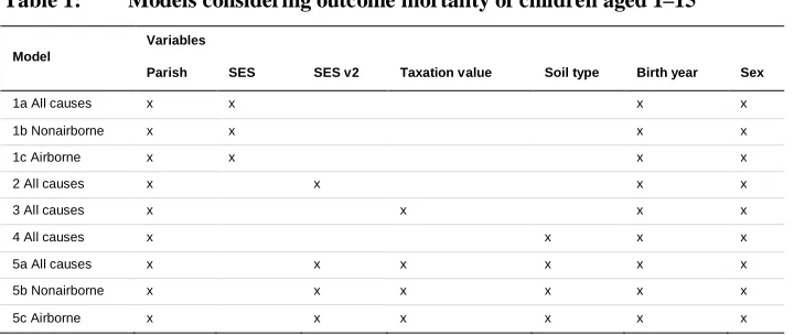
estimate simple models focusing on parish of residence and socioeconomic status. Thereafter, we extend these models with the inclusion of the soil type variable in order to study whether soil type may explain some of the previously found mortality differences between the parishes in our study area. Moreover, models 1b and 5b analyse the mortality risk from nonairborne/unspecified diseases in order to better identify deaths that could have been caused by the lack of nutrition, whereas models 1c and 5c analyse the mortality risk from only airborne diseases to identify deaths that could have been caused by increased exposure to highly virulent diseases (cf. Table 2).
Table 1: Models considering outcome mortality of children aged 1–15
Model
Variables
Parish SES SES v2 Taxation value Soil type Birth year Sex
1a All causes x x x x
1b Nonairborne x x x x
1c Airborne x x x x
2 All causes x x x x
3 All causes x x x x
4 All causes x x x x
5a All causes x x x x x x
5b Nonairborne x x x x x x
5c Airborne x x x x x x
Notes:Variables included in the models are marked by the letter x.
Likelihood Ratio (LR) tests on models 1a and 3–5a analyse whether the addition of variables in the extended models improve model fit. We run a separate model for infants as a sensitivity analysis to test if their mortality is affected by soil type.3 Moreover, except for model 1b and 1c, the models are also estimated separately for children of labourers and small- and medium-scale farmers. For models 1a and 3–5a, Cox proportional hazard models are used (Therneau and Grambsch 2000), whereas a competing-risks regression model is used for models 1b-c and 5b-c (Fine and Gray 1999). All Cox proportional hazard models also included a shared frailty component to measure the proportion of unobserved characteristics shared between members of the same household. That is, thetas were obtained to measure within-household variation in
3
mortality. Because of the spatial autocorrelation4 for the soil types, we also tested models with property units as a shared frailty (not reported here), but this did not change our results. Tests based on Schoenfeld residuals were conducted after each model to test the proportionality of the hazards, and no violations in this assumption were found in the main explanatory variables.
Because the studied age group of 1–15 years may be heterogeneous, as a sensitivity analysis we also studied separately the age groups 1–4 and 5–15. We first performed ANOVA tests, which revealed that there were no statistical significant differences in the causes of deaths of children of the two age groups (both for all children and for the two socioeconomic groups). We also estimated separate Cox proportional hazard models for the two age groups. Although the hazard ratios and p-values varied somewhat, the patterns remained consistent to results of the model that focused on children aged 1–15 (Tables 5–6, Model 5a). Finally, we observed a correlation between some of the soil type groups and parishes and, in some degree, between soil type and SES, which indicates a possible redundancy between the variables. There were also overlaps between parish and SES. That is, freeholders mainly resided in Hög, Kävlinge, and Kågeröd, whereas tenants commonly lived in Sireköpinge, Halmstad, and Kågeröd; the groups considered in the newly introduced measure of SES (SES v2), landless and semilandless, however, were more equally distributed among the parishes. We tested for multicollinearity by estimating linear regressions including soil and parish and thereafter checked the variance inflation factor (VIF). These tests showed no indication of such multicollinearity issues between the variables. Hence, the variables likely explain different parts of the variations in mortality in the model.
5.3 Descriptive statistics
Table 2 shows the distribution of the children’s time at risk in percentage among the categorical variables considered in this study, and the average values of the continuous variables. The values for the taxation value represent only those individuals that had a value higher than zero. As seen in the table, farmers have a higher taxation value. The unlinked soil type group represents the share of individuals that for parts of, or for their whole life course, could not be linked to a property unit. These individuals belonged
4
primarily to the landless class and some of them were the poorest people, who wandered about between farms and other lodgings. Consequently, it has been difficult to link them to a household or to a property unit.
Table 2: Distribution of the time at risk in person-years on the independent variables used in this study, farmer and labourer children, age 1–15, Scania, 1850–1914
All Small- and medium-scale
farmers Labourers
% % %
Soil type
Clayey till 75–100% 20.43 22.28 20.60 Clayey till 50–75% 20.21 23.38 19.99 Clay-till/clay 50–100% 21.81 29.20 19.69 Sandy soils 50–100% 17.10 15.24 17.43
Mixed 9.58 9.91 8.89
Unlinked 10.88 13.40
SES
Freeholders 9.56 33.68 Tenants 15.06 50.41
Semilandless 18.10 15.91 20.22
Landless 57.28 79.78
SES v2
Large farmers 6.90 Small-medium farmers 21.13 Labourers 71.98
Parish
Hög 9.16 15.14 7.21
Kävlinge 8.32 9.18 7.61
Halmstad 19.41 24.28 18.98
Sireköpinge 27.85 27.14 28.26
Kågeröd 32.25 24.26 37.94
Sex
Female 47.92 48.03 48.11
Male 52.08 51.97 51.89
Birth year
(average and min–max)
1872.75 (1835–1912) 1871.43 (1835–1912) 1873.03 (1835–1912) Taxation value (average and min–max)
0.27 (0.01–3.00) 0.15 (0.02–0.4) 0.01 (0.00–0.03)
Individuals 15,485 3,235 12,900
Deaths 997 207 744
gastrointestinal diseases, psychiatric diagnoses, congenital heart disease, and kidney suffering. Table 3 shows that the largest groups of causes of death for both classes were the nonspecified diseases, followed by the airborne diseases. The share of causes of deaths is almost identical between the two groups. Some differences, however, are observed; e.g., the labourers’ children have a higher share of accidents and crimes, as well as food- and waterborne diseases.
To create sufficiently large groups for the cause-specific models (presented in Tables 4–6), we study the mortality where the outcome is from either nonairborne/unspecified diseases or airborne diseases. Such classification has two limitations that may introduce biases in the analyses. First, the nonairborne/unspecified group is heterogeneous, with a very large share of cases not being specified. Second, diseases such as different types of respiratory infections, measles, and tuberculosis cause approximately half of the deaths within the group airborne infectious diseases, for which the risk of infection may be influenced by an individual’s nutritional status (cf. e.g., Bellagio conference authors 1985). Therefore, we cannot estimate models for causes of deaths that are either explicitly linked to nutrition or not linked to nutrition (i.e., highly virulent diseases). Hence, the results from the cause-specific models have to be interpreted with care. Despite this limitation, analysing the mortality using such models is, nonetheless, a first step towards trying to better understand the influence of soil type, as an indicator of nutrition, on child mortality.
Table 3: Mortality by cause of death, farmer and labourer children, age 1–15, Scania, 1850–1914. Total and relative frequencies
Small- and medium-scale farmers Labourers
Total % Total %
Airborne infectious diseases 61 29.47 221 29.70 Food- and waterborne infectious
diseases
8 3.86 50 6.72
Other infectious diseases 2 0.97 4 0.54 Cardiovascular diseases and
diabetes
2 0.97 9 1.21
Accidents, crimes, etc. 1 0.48 21 2.82
Cancer 1 0.48 5 0.67
Other specified noninfectious diseases
23 11.11 79 10.62
Not specified 109 52.66 355 47.72 Total nonairborne infectious
diseases/not specified
146 70.53 523 70.30
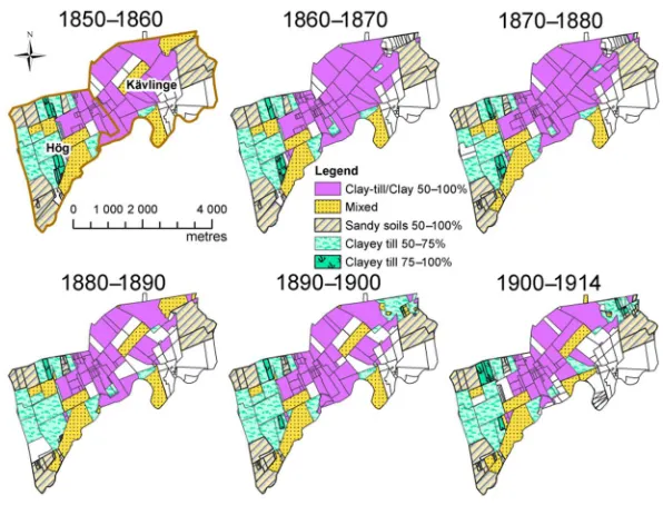
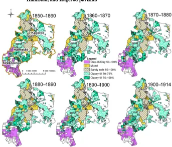
Figures 2 and 3 show the spatial distribution of the soil type groups for all children aged 1–15. Note that the maps show all the property units that ever existed during each 10-year period. This means that some property units may overlay each other on the map, and that some property units may have existed for only a short period. Moreover, the empty areas in white represent property units where no individuals are linked. The large white area in Kävlinge parish represents the urban area that we excluded in the analyses. As regards to the soil type distribution, clay-till/clay soils dominate in the middle of Kävlinge and Hög, as well as in the southern parts of Sireköpinge (mainly clay-tills). Halmstad and Kågeröd are dominated by areas with large proportions of clayey till and sandy soils. Note also that the soil type variable seems to change for some property units through time. This is because the property units change size (e.g., because of subdivisions) through time and that larger property units are sometimes overlaid by smaller property units in the map. Hence, although the soil type is static, the soil type variable sometimes varies in time.
Figure 2: Distribution of the soil variable based on the % of the spatial coverage of soil types in each property unit in Hög and Kävlinge parishes
Figure 3: Distribution of the soil variable based on the % of the spatial coverage of soil types in each property unit in Sireköpinge, Halmstad, and Kågeröd parishes
Note:The white areas represent property units where no individuals (children aged 1–15) are linked.
Kågeröd. Lastly, we observe mortality differences between the soil types groups, in which children living in property units with mixed soil types experience the lowest mortality, whereas the unlinked children have the highest risk of dying.
Figure 4: Nelson–Aalen cumulative hazards by SES, SES v2, parish of residence, and soil type, ages 1–15, 1850–1914
6. Results
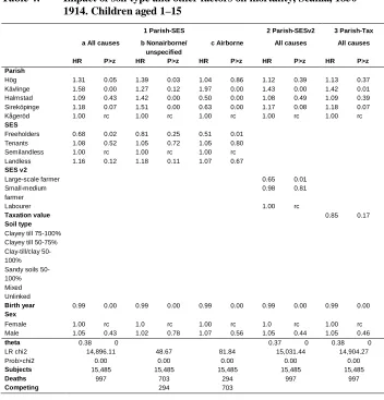
paper). Large mortality differences between the nonairborne/unspecified and airborne diseases for the parishes are also observed (Models 1b–c and 5b–c).
The freeholders (when considering the first SES classification) and large-scale farmers (when considering the second SES classification) experience a relatively much lower risk of death compared to the other social groups. However, in the cause-specific models, this effect is only statistical significant in the models estimated for airborne diseases. Hence, these results may indicate that some of the airborne infectious diseases are nutrition-dependent, or that the upper classes were less exposed to highly virulent diseases. Moreover, year of birth had a beneficial effect on children: an increase of one in year of birth decreases the mortality risk by 1% (model 5a).
Table 4: Impact of soil type and other factors on mortality, Scania, 1850– 1914. Children aged 1–15
1 Parish-SES 2 Parish-SESv2 3 Parish-Tax
a All causes b Nonairborne/ unspecified
c Airborne All causes All causes
HR P>z HR P>z HR P>z HR P>z HR P>z
Parish
Hög 1.31 0.05 1.39 0.03 1.04 0.86 1.12 0.39 1.13 0.37 Kävlinge 1.58 0.00 1.27 0.12 1.97 0.00 1.43 0.00 1.42 0.01 Halmstad 1.09 0.43 1.42 0.00 0.50 0.00 1.08 0.49 1.09 0.39 Sireköpinge 1.18 0.07 1.51 0.00 0.63 0.00 1.17 0.08 1.18 0.07 Kågeröd 1.00 rc 1.00 rc 1.00 rc 1.00 rc 1.00 rc
SES
Freeholders 0.68 0.02 0.81 0.25 0.51 0.01 Tenants 1.08 0.52 1.05 0.72 1.05 0.80 Semilandless 1.00 rc 1.00 rc 1.00 rc Landless 1.16 0.12 1.18 0.11 1.07 0.67
SES v2
Large-scale farmer 0.65 0.01 Small-medium
farmer
0.98 0.81
Labourer 1.00 rc
Taxation value 0.85 0.17
Soil type
Clayey till 75-100% Clayey till 50-75% Clay-till/clay 50-100% Sandy soils 50-100% Mixed Unlinked
Birth year 0.99 0.00 0.99 0.00 0.99 0.00 0.99 0.00 0.99 0.00
Sex
Female 1.00 rc 1.0 rc 1.00 rc 1.0 rc 1.00 rc Male 1.05 0.43 1.02 0.78 1.07 0.56 1.05 0.44 1.05 0.46
theta 0.38 0 0.37 0 0.38 0
LR chi2 14,896.11 48.67 81.84 15,031.44 14,904.27 Prob>chi2 0.00 0.00 0.00 0.00 0.00
Subjects 15,485 15,485 15,485 15,485 15,485
Deaths 997 703 294 997 997
Competing 294 703
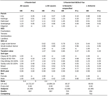
Table 4: (Continued)
4 Parish-Soil 5 Parish-Soil-SESv2-Tax
All causes a All causes b Nonairb./ unspecified
c Airborne
HR P>z HR P>z HR P>z HR P>z
Parish
Hög 1.17 0.26 1.16 0.27 1.28 0.10 0.88 0.56 Kävlinge 1.43 0.01 1.42 0.01 1.23 0.20 1.67 0.01 Halmstad 1.13 0.27 1.11 0.32 1.45 0.00 0.51 0.00 Sireköpinge 1.23 0.05 1.22 0.06 1.56 0.00 0.66 0.02 Kågeröd 1.00 rc 1.00 rc 1.00 rc 1.00 rc
SES Freeholders Tenants Semilandless Landless SES v2
Large-scale farmer 0.62 0.01 0.78 0.24 0.44 0.02 Small-medium farmer 0.99 0.89 1.00 0.96 1.01 0.95 Labourer 1.00 rc 1.00 rc 1.00 rc
Taxation value 1.07 0.64 0.85 0.27 1.35 0.20
Soil type
Clayey till 75-100% 1.00 rc 1.00 rc 1.00 rc 1.00 rc Clayey till 50-75% 1.20 0.10 1.20 0.10 1.05 0.68 1.58 0.02 Clay-till/clay 50-100% 1.04 0.77 1.04 0.74 0.95 0.69 1.23 0.35 Sandy soils 50-100% 1.09 0.48 1.10 0.45 1.08 0.55 1.21 0.39 Mixed 0.91 0.52 0.91 0.54 0.79 0.15 1.35 0.23 Unlinked 1.23 0.11 1.28 0.07 1.04 0.77 1.62 0.04
Birth year 0.99 0.00 0.99 0.00 0.99 0.00 0.99 0.00
Sex
Female 1.00 rc 1.00 rc 1.00 rc 1.00 rc Male 1.05 0.45 1.05 0.42 1.02 0.80 1.08 0.53
theta 0.4 0 0.4 0
LR chi2 14,721.67 14,894.24 49.37 88.93 Prob>chi2 0.00 0.00 0.00 0.00
Subjects 15,485 15,485 15,485 15,485
Deaths 997 997 703 294
Competing 294 703
Notes:HR = hazard ratio, rc =reference category, person-years at risk: 96,952.
Table 5 and Figure 5 show the results from the separate models for children to small- and medium-scale farmers. (Note: Figure 5 shows only the effects from the soil type and parish variables.) A relatively strong effect of soil types and taxation value on mortality is revealed, which is consistent across the models.5 Thus, the results indicate a possible effect of nutrition, through soil type and taxation value, on the mortality of the
5
farmers’ children. Moreover, we observe no significant mortality differences between the parishes for this group of children. However, in the cause-specific model for nonairborne/unspecified diseases (model 5b), children residing in Halmstad and Sireköpinge show higher hazards of death. Overall, children residing in areas with very high proportions of clayey till (75–100% coverage) experience a lower risk of dying compared to children residing in areas with other soil types. In particular, children residing in property units with a spatial coverage of 50–75% clayey till or with mixed soils have approximately twice as high a hazard of death as children residing in property units with a spatial coverage of 75–100% clayey till (models 4 and 5a). The magnitude of the effects, as well as the statistical significance, of the soil types decreases in the model that considers as outcome mortality from nonairborne or unspecified diseases (model 5b), although the pattern of the effects remains constant. An exception is the effects of the group sandy soils 50–100%, for which the effect becomes stronger and statistically significant at the 5% level. That is, the hazard of death from nonairborne/unspecified diseases for children residing in farms with soil type sandy soils 50–100% is 96% higher relative to children living in farms with soil type clayey till 75–100%. Thus, in this cause-specific model we can observe a trend from lower hazards of mortality for children living in areas with large proportions of fertile clayey till soils to higher hazards of mortality for children living in areas with less fertile sandy soils.
Figure 5: Impact of soil type and parish on child mortality, Scania, 1850–1914. Small- and medium-scale farmers, aged 1–15
Table 5: Impact of soil type and other factors on child mortality, Scania, 1850–1914. Small- and medium-scale farmers, aged 1–15
1 Parish-SES 3 Parish-Tax 4 Parish-Soil 5 Parish-Soil-Tax
All causes All causes All causes a All causes b Nonairborne/ unspecified
HR P>z HR P>z HR P>z HR P>z HR P>z
Parish
Hög 0.87 0.61 0.79 0.39 0.86 0.60 0.77 0.36 0.96 0.90 Kävlinge 0.93 0.82 0.84 0.59 1.01 0.99 0.89 0.74 1.04 0.92 Halmstad 1.13 0.60 1.01 0.98 1.05 0.85 0.94 0.79 1.75 0.04 Sireköpinge 1.12 0.63 0.96 0.88 1.13 0.64 0.97 0.91 1.66 0.07 Kågeröd 1.00 rc 1.00 rc 1.00 rc 1.00 rc 1.00 rc
Taxation value 0.18 0.05 0.16 0.04 0.23 0.11
Soil type
Clayey till 75-100% 1.00 rc 1.00 rc 1.00 rc Clayey till 50-75% 1.91 0.01 1.98 0.01 1.67 0.04 Clay-till/clay 50-100% 1.32 0.30 1.39 0.22 1.14 0.64 Sandy soils 50-100% 1.49 0.18 1.63 0.10 1.96 0.04 Mixed 2.11 0.01 2.11 0.01 1.57 0.14 Unlinked
Birth year 0.99 0.00 0.99 0.00 0.99 0.00 0.99 0.00 0.98 0.00
Sex
Female 1.00 rc 1.00 rc 1.00 rc 1.00 rc 1.00 rc Male 1.28 0.09 1.28 0.09 1.29 0.08 1.29 0.08 1.21 0.26
theta 0.71 0.00 0.65 0.00 0.61 0.00 0.54 0.00
LR chi2 2,855.50 2,926.66 2,906.05 2,989.27 29.34 Prob>chi2 0.00 0.00 0.00 0.00 0.00
Subjects 3,235 3,235
Deaths 207 146
Competing 61
Person-years at risk 20,485 20,485
Note:HR = hazard ratio, rc =reference category
Whereas the effect of the taxation value on mortality may seem relatively large, it represents the increase of 1 mantal, which is a large unit increase (the small- and medium-scale farmers have a mantal between 0.02 and 0.4). An increase of 0.1 of a
mantal decreases the mortality risk by 8.4% (model 5a). Moreover, male children had a higher mortality risk compared to female children (e.g., 28.8% in model 5a) (P<0.1), and the shared frailty within the households was high: 53.9% in the model including soil type and taxation value (model 5a).
For the labourers’ children, we observe no significant mortality differences between the soil type groups representing areas covered by high proportions of a specific soil type (Figure 6, Table 6).6 Also, no beneficial effect of taxation value is
6
found. However, labourers’ children residing in areas with mixed soils (foremost a mix of clayey till, clay/clay-till, and sandy soils) experience in general a lower risk of dying compared to children residing in areas with other soil type groups. Moreover, the mortality differences observed in Figure 6 and Table 6 between the parishes for the labourers’ children (model 1) are similar to the ones found in Table 4. This adheres to both the parish differences found for all-cause mortality as well as the large differences between the cause-specific models estimated for nonairborne/unspecified and airborne diseases. Note, however, that when including the soil type variable in the models considering all-cause mortality, there are no longer any statistically significant effects from Sireköpinge parish. Moreover, even though the urban area of Kävlinge was excluded in the analyses, children living in Kävlinge parish have a significantly higher mortality compared to the reference category in all models, except for the cause-specific model for nonairborne/unspecified diseases. This indicates that children also living outside the urban area in Kävlinge have an increased hazard of death from airborne diseases. Finally, the shared frailty within the households was generally smaller compared to the farmers’ children: between 33.6% and 35.3% (Table 6: models 1, 3–4, 5a).
Figure 6: Impact of soil type and parish on child mortality, Scania, 1850–1914. Labourers, aged 1–15
Table 6: Impact of soil type and other factors on child mortality, Scania, 1850–1914. Labourers, aged 1–15
1 Parish-SES 3 Parish-Tax 4 Parish-Soil 5 Parish-Soil-Tax
All causes All causes All causes a All causes b Nonairborne/
unspecified c Airborne
HR P>z HR P>z HR P>z HR P>z HR P>z HR P>z
Parish
Hög 1.26 0.14 1.25 0.15 1.26 0.16 1.26 0.17 1.30 0.15 1.01 0.98 Kävlinge 1.66 0.00 1.66 0.00 1.58 0.00 1.57 0.00 1.26 0.20 2.05 0.00 Halmstad 1.06 0.63 1.06 0.65 1.08 0.51 1.08 0.53 1.35 0.02 0.53 0.01 Sireköpinge 1.25 0.03 1.25 0.03 1.22 0.10 1.21 0.11 1.48 0.00 0.79 0.23 Kågeröd 1.00 rc 1.00 rc 1.00 rc 1.00 rc 1.00 rc 1.00 rc
Taxation value 1.15 0.40 1.24 0.23 0.91 0.55 1.77 0.08
Soil type
Clayey till 75-100% 1.00 rc 1.00 rc 1.00 rc 1.00 rc Clayey till 50-75% 1.07 0.61 1.07 0.60 0.94 0.64 1.46 0.10 Clay-till/clay 50-100% 1.08 0.57 1.08 0.56 1.01 0.95 1.16 0.55 Sandy soils 50-100% 1.09 0.53 1.09 0.54 1.05 0.73 1.27 0.35 Mixed 0.70 0.05 0.70 0.05 0.60 0.02 1.02 0.96 Unlinked 1.15 0.32 1.21 0.20 1.02 0.92 1.43 0.17
Birth year 0.99 0.00 0.99 0.00 0.99 0.00 0.99 0.00 0.99 0.00 0.98 0.08
Sex
Female 1.00 rc 1.00 rc 1.00 rc 1.00 rc 1.00 rc 1.00 rc Male 0.99 0.88 0.99 0.89 0.99 0.91 0.99 0.92 0.97 0.68 1.00 0.99
theta 0.34 0.00 0.35 0.00 0.34 0.00 0.35 0.00
LR chi2 11,255.68 11,240.97 11,201.69 11,155.59 33.65 66.75 Prob>chi2 0.00 0.00 0.00 0.00 0.00 0.00
Subjects 12,900 12,900 12,900
Deaths 744 523 221
Competing 221 523
Person-years at risk 69,782 69,782 69,782
Notes:HR = hazard ratio, rc =reference category
7. Discussion and conclusions
By combining detailed geographic information on residential histories with information on soil type for each property unit, we were able to analyse the impacts of soil type on child mortality (ages 1–15) for the period 1850–1914. The results indicate that soil type primarily affected the mortality of the children of farmers. Particularly, these children experienced relatively lower mortality when living in property units covered by very high proportions of clayey till. We observed some effects of soil type for the labourers’ children; however, in contrast to the farmers’ children, they had a lower mortality when residing in property units covered by mixed soils (foremost constituted of clayey till, clay-till/clay, and sandy soils). This soil type, however, is a small heterogeneous category that may possibly correlate with other unobserved factors that are not considered in the models. Therefore, the results indicate some support for our first hypothesis; i.e., that soil type is a measure for nutrition of children of farmers. That is, certain soil types may have influenced the farm-level production pattern and the quantity and quality of the output, which in turn affected the nutritional level of the farmers’ children and thus their likelihood of dying. Moreover, we found little support for our second hypothesis, which predicted that soil was instead a measure of exposure to virulent diseases, because soil types did not affect the mortality of the two groups equally. Consequently, the results indicate the relatively important role of nutrition as a mortality predictor for the farmers’ children, which is in line with previous research on the link between nutrition and disease outcomes in preindustrial societies (e.g., McKeown 1976; Fogel 1994, 2004; Puleston and Tuljapurkar 2008; Floud et al. 2011). Note, however, that we have not been able to estimate models that explicitly describe diseases that are either dependent or not dependent on nutrition. In addition, the group containing the farmers’ children is small. Therefore, the results of this study have to be interpreted with care and further research is needed to better study the relationship between nutrition and the risk of dying in a preindustrial society.
A possible explanation for the different effects of soil on mortality for the farmers’ children is that clayey till was in general more fertile than sandy soils and more manageable than heavy clay-till and clay soils. For example, in the cause-specific model for nonairborne/unspecified diseases, a trend can be observed from lower risks of mortality for children living in farms with more fertile soils (clayey till) to higher risks of mortality for children living in farms with less fertile soils (sandy soils). However, market and technological developments likely affected the suitability of a soil type for agriculture. Some soils may have been more suited for specific crops, which was likely influenced by the current market demand for these crops. For example, the rising popularity of new crops such as sugar beets, which began to be cultivated in the 1890s in the five parishes (BiSOS 1892), as well as the increased use of both natural and artificial fertilizers (Morell 2011) probably influenced the importance of some soil types. For example, well-drained medium to slightly fine-textured soils are good soils for sugar beets (FAO 2015). Hence, lands with large proportions of clayey tills and, possibly, clay-tills may have been suited for such crops. However, sugar beets are also sensitive to the pH value in the soil, which may vary across areas regardless of the soil type (FAO 2015). Moreover, the agricultural suitability of heavy clay soils may have increased in the latter part of our study period because of the improvements in drainage and the use of better tools (Morell 2011; Bohman 2010). To study the impact of such technological developments, we could have divided the analysis into two periods; however, this was not possible because it resulted in an insufficient sample size. Lastly, the shared frailty component, which measures unobserved characteristics within the household-level, was high in the models estimated for the farmers’ children (54%). This suggests that their mortality is affected also by other unobserved factors that have not been considered in this study.
Some research indicates that soil affects infant mortality; e.g., Munro et al. (1997) found that wards dominated by wet soils had a relatively high infant mortality. In contrast, we found no effect of soil types on mortality for infants in the models that we conducted as a sensitivity analysis. However, both the demographic and geographic data used in the study by Munro et al. (1997) were on an aggregate level, whereas this study uses longitudinal microlevel data over a smaller area. Furthermore, we did not classify the soils based on their wetness; therefore, the results may not be comparable.
Although this work brings new knowledge to our understanding of mortality in the past, it is not free from limitations. One such limitation concerns the individuals that for parts of or for their whole life-course have not been linked to a property unit. Many of the poorest families belonged to this group, families with no fixed addresses and who often resided in poorhouses. They were a vulnerable group with relatively high mortality (Table 4). Such individuals are important to consider in the analyses to avoid creating a potential risk of a bias in the results. Including them as a separate group (unlinked) in the soil type variable was one way to handle this problem. However, this was only possible in the less extended models for the labourers’ children.
Another limitation is the correlation that exists between some of the soil type groups and parishes (see Figures 2–3) and, to some degree, between soil type and SES. Thus, there is some redundancy between the variables. The multicollinearity tests, however, showed no serious indications of such concerns; therefore, the variables likely explain different parts of the variations in mortality in the model. Connected to this issue is also the spatial autocorrelation of the soil types. To overcome such limitation, we estimated models that included a frailty component for a geographical unit; i.e., the property units (not shown in this paper). This did not change our main results in any substantial way. However, a more proper way to study this would be to use a model that also takes into account the neighbouring areas and thus controls for the spatial autocorrelation; for example, a Cox proportional hazard model with spatially shared frailties (Darmofal 2009).
Moreover, the models on cause-specific mortality were limited by the large share of unspecified deaths and by the fact that the two groups considered, nonairborne/unspecified and airborne, may not necessarily represent a proper distinction between causes of death that may and may not be related to nutrition. However, we see these estimations as a first and preliminary step to better understand the role of nutrition on mortality. Further research that looks in more depth into different causes of death is required.
Lastly, the findings of this work could be extended by making some additional improvements to the models. Foremost it is possible to use various soil assessment models or specific crop yield models to more accurately estimate farm-level productivity (e.g., Brunt 2004; Steduto et al. 2009). In these models, we could include information such as detailed elevation data and topographic wetness indexes (TWI).
Despite the abovementioned limitations, this is, to our knowledge, the first longitudinal study at the microlevel that analyses the effects of soil type on mortality in a historical rural society, and we therefore contribute to the literature on the role of nutrition on the risk of dying in a preindustrial society.
8. Acknowledgements
References
Abrahams, P.W. (2002). Soils: Their implications to human health.Science of the Total Environment291(1‒3): 1‒32.doi:10.1016/S0048-9697(01)01102-0.
Allen, R.C. (2008). The nitrogen hypothesis and the English agricultural revolution: A biological analysis. Journal of Economic History 68(1): 182‒210.
doi:10.1017/S0022050708000065.
Bellagio conference authors (1985). The relationship of nutrition, disease and social conditions: A graphical presentation. In Rotberg, R. and Rabb, T. (eds.).Hunger and history. The impact of changing food production and consumption patterns on society. New York: Cambridge University Press: 304‒308.
Bengtsson, T. (1999). The vulnerable child. Economic insecurity and child mortality in pre-industrial Sweden: A case study of Västanfors, 1757–1850. European Journal of Population15(2): 117‒151.
Bengtsson, T. (2004). Mortality and social class in four Scanian parishes, 1766–1865. In: Bengtsson, T., Campbell, C., and Lee, J.Z. (eds.). Life under pressure: Mortality and living standards in Europe and Asia, 1700–1900. London: MIT Press: 135‒171.
Bengtsson, T. and Broström, G. (2010). Mortality crises in rural southern Sweden 1766–1860. In: Kurosu, S., Bengtsson, T., and Campbell, C. (eds).Demographic responses to economic and environmental crises. Kashiwa: Reitaku University Press: 1‒16.
Bengtsson, T. and Dribe, M. (2010). Quantifying the family frailty effect in infant and child mortality by using Median Hazard Ratio (MHR). Historical Methods: A Journal of Quantitative and Interdisciplinary History43(1): 15‒27.
Bengtsson, T. and Dribe, M. (2011). The late emergence of socioeconomic mortality differentials: A micro-level study of adult mortality in southern Sweden, 1815– 1968. Explorations in Economic History 48(3): 389‒400.
doi:10.1016/j.eeh.2011.05.005.
Bengtsson, T. and Lindstrom, M. (2000). Childhood misery and disease in later life: The effects on mortality in old age of hazards experienced in early life, southern Sweden, 1760–1894. Population Studies 54(3): 263‒277.
doi:10.1080/713779096.
Bengtsson, T. and Lundh, C. (1994). La mortalité infantile et post-infantile dans les pays Nordiques avant 1900.Annales de Démographie Historique 1994(1): 23– 43.
Bengtsson, T. and van Poppel, F. (2011). Socioeconomic inequalities in death from past to present: An introduction.Explorations in Economic History48(3): 343‒356.
BiSos (1892). Bidrag till Sveriges officiella statistik. N, Jordbruk och boskapsskötsel. Stockholm: Statistiska centralbyrån, P.A. Norstedt & söner.
Bohman, M. (2010). Bonden, bygden och bördigheten: Produktionsmönster och utvecklingsvägar under jordbruksomvandlingen i Skåne ca 1700–1870. [PhD thesis]. Lund: Lund University, Department of Economic History.
Brändström, A. (1984). “De kärlekslösa mödrarna”: Spädbarnsdödligheten i Sverige under 1800-talet med särskild hänsyn till Nedertorneå. [PhD thesis]. Umeå: Umeå University.
Brändström, A., Edvinsson, S., and Rogers, J. (2002). Illegitimacy, infant feeding practices and infant survival in Sweden, 1750–1950: A regional analysis.Hygiea Internationalis 3(1): 13–52.doi:10.3384/hygiea.1403-8668.023113.
Brunt, L. (2004). Nature or nurture? Explaining English wheat yields in the industrial revolution, c. 1770. Journal of Economic History 64(1): 193‒225.
doi:10.1017/S0022050704002657.
Claësson, O. (2009). Geographical differences in infant and child mortality during the initial mortality decline: Evidence from southern Sweden, 1749–1830. [Lic. thesis]. Lund: Lund University, Department of Economic History.
Darmofal, D. (2009). Bayesian spatial survival models for political event processes.
American Journal of Political Science 53(1): 241‒257. doi:10.1111/j.1540-5907.2008.00368.x.
Dobson, M.J. (1994). Malaria in England: A geographical and historical perspective.
Parassitologia36(1‒2): 35‒60.
Dribe, M. (2000). Leaving home in a peasant society. Economic fluctuations, household dynamics and youth migration in southern Sweden, 1829–1866. [PhD thesis]. Lund: Lund University, Department of Economic History.
Dribe, M. and Bengtsson, T. (1997). Economy and demography in western Scania, Sweden, 1650–1900.Kyoto: International research center for Japanese studies
(EAP working series paper no.10).
Dribe, M., Olsson, M., and Svensson, P. (2011). Production, prices and mortality: Demographic response to economic hardship in rural Sweden, 1750–1860.
Paper presented at the meetings of the European Historical Economics Society, Dublin, Ireland, September 2–3, 2011.
Eriksson, J., Nilsson, I., Simonsson, M., and Wiklander, L. (2005). Wiklanders marklära. Lund: Studentlitteratur.
Food and Agriculture Organization of the United Nations (FAO) (2015). Crop Water Information: Sugarbeet [electronic resource]. Rome: FAO Water Development and Management Unit. http://www.fao.org/nr/water/cropinfo_sugarbeet.html
Fine, J.P. and Gray, R.J. (1999). A proportional hazards model for the subdistribution of a competing risk. Journal of the American statistical association 94(446): 496‒509.doi:10.1080/01621459.1999.10474144.
Fischer, G., van Velthuizen, H.T., Shah, M.M., and Nachtergaele, F.O. (2002). Global agro-ecological assessment for agriculture in the 21st century: Methodology and results. Laxenburg: IIASA: 157 pp.
Floud, R., Fogel, R.W., Harris, B., and Hong, S.C. (2011).The changing body: Health, nutrition, and human development in the western world since 1700. Cambridge: Cambridge University Press.doi:10.1017/CBO9780511975912.
Fogel, R. (1994). Economic growth, population theory and physiology: The bearing of long-term processes on the making of economic policy. American Economic Review 84(3): 369‒395.doi:10.3386/w4638.
Fogel, R. (2004). The escape from hunger and premature death, 1700–2100: Europe, America and the Third World. Cambridge: Cambridge University Press.
doi:10.1017/CBO9780511817649.
Gadd, C.-J. (1983). Järn och potatis: Jordbruk, teknik och social omvandling i Skaraborgs län 1750–1860. [PhD thesis]. Göteborg: University of Gothenborg, Department of Economic History.
Gadd, C.-J. (2011). The agricultural revolution in Sweden, 1700–1870. Lund: Nordic Academic Press.
Goldstein, E.J.C., Katona, P., and Katona-Apte, J. (2008). The interaction between nutrition and infection. Clinical Infectious Diseases 46(10): 1582‒1588.
doi:10.1086/587658.
Gregory, I.N. (2008). Different places, different stories: Infant mortality decline in England and Wales, 1851–1911. Annals of the Association of American Geographers98(4): 773‒794.doi:10.1080/00045600802224406.
Hawley, J.K. (1985). Assessment of health risk from exposure to contaminated soil.
Risk Analysis5(4): 289‒302.doi:10.1111/j.1539-6924.1985.tb00185.x.
Hedefalk, F. (2016). Life paths through space and time: Adding the micro-level geographic context to longitudinal historical demographic research. [PhD thesis]. Lund: Lund University, Department of Physical Geography and Ecosystem Science.
Hedefalk, F., Harrie, L., and Svensson, P. (2014). Extending the Intermediate Data Structure (IDS) for longitudinal historical databases to include geographic data.
Historical Life Course Studies 1: 27‒46.
Hedefalk, F., Harrie, L., and Svensson, P. (2015). Methods to create a longitudinal integrated demographic and geographic database on the micro-level. A case study of five Swedish rural parishes, 1813–1914.Historical Methods: A Journal of Quantitative and Interdisciplinary History 48(3): 153‒173.
doi:10.1080/01615440.2015.1016645.
Hedefalk, F., Pantazatou, K., Quaranta, L., and Harrie, L. (2016). Importance of the geocoding level for historical demographic analyses: A case study of rural parishes in Sweden, 1850–1914. Lund: Lund University, Department of Physical Geography and Ecosystem Science, and Centre for Economic Demography.
Hedefalk, F., Svensson, P., and Harrie, L. (2017). Spatiotemporal historical datasets at micro-level for geocoded individuals in five Swedish parishes, 1813–1914.
Jaenicke, E. and Lengnick, L. (1997). A soil–quality index and its relationship to efficiency and productivity growth measures: Two decompositions. American Journal of Agricultural Economics79(5): 1702‒1702.
Kintner, H.J. (1985). Trends and regional differences in breastfeeding in Germany from 1871 to 1937. Journal of Family History 10(2): 163‒182.
doi:10.1177/036319908501000203.
Lazuka, V., Quaranta, L., and Bengtsson, T. (2016). Fighting infectious disease: Evidence from Sweden, 1870–1940.Population and Development Review 42(1): 27‒52.doi:10.1111/j.1728-4457.2016.00108.x.
Lee, C.T. and Tuljapurkar, S. (2008). Population and prehistory I: Food-dependent population growth in constant environments. Theoretical Population Biology
73(4): 473‒482.doi:10.1016/j.tpb.2008.03.001.
Lindgren, E. and Jaenson, T.G. (2006). Fästing-och myggöverförda infektionssjukdomar i ett kommande, varmare klimat i Sverige.Ent. Tidskr127: 21‒30.
Lundh, C. and Olsson, M. (2011). Contract-workers in Swedish agriculture, c. 1890s– 930s: A comparative study of standard of living and social status.Scandinavian Journal of History36(3): 298‒323.doi:10.1080/03468755.2011.582620.
Mayagaya, V.S., Nkwengulila, G., Lyimo, I.N., Kihonda, J., Mtambala, H., Ngonyani, H., Russel, L.T., and Ferguson, H.M. (2015). The impact of livestock on the abundance, resting behaviour and sporozoite rate of malaria vectors in southern Tanzania.Malaria Journal 14(17): 1‒13.doi:10.1186/s12936-014-0536-8.
McKeown, T. (1976).The modern rise of population. London: Arnold.
McKeown, T., Brown, R.G., and Record, R.G. (1972). An interpretation of the modern rise of population in Europe. Population Studies 26: 345‒382.
doi:10.2307/2173815.
Morell, M. (2011). Agriculture in industrial society, 1870–1945. In: Myrdal, J. and Morell, M. (eds.).The agrarian history of Sweden: From 4000 BC to AD 2000. Lund: Nordic Academic Press: 165–213.
Munro, L.J.A., Penning-Rowsell, E.C., Barnes, H.R., Fordham, M.H., and Jarrett, D. (1997). Infant mortality and soil type: A case study in south-central England.
Oliver, M.A. and Gregory, P.J. (2015). Soil, food security and human health: A review.
European Journal of Soil Science66(2): 257‒276.doi:10.1111/ejss.12216.
Oris, M., Derosas, R., and Breschi, M. (2004). Infant and child mortality. In: Bengtsson, T., Campbell, C., and Lee, J.Z. (eds.).Life under pressure: Mortality and living standards in Europe and Asia, 1700–1900. London: MIT Press: 359‒ 398.
Patz, J.A., Strzepek, K., Lele, S., Hedden, M., Greene, S., Noden, B., Hay, S., Kalkstein, L., and Beier, J.C. (1998). Predicting key malaria transmission factors, biting and entomological inoculation rates, using modelled soil moisture in Kenya. Tropical Medicine and International Health 3(10): 818‒827.
doi:10.1046/j.1365-3156.1998.00309.x.
Pettersson, L. (1989). Riksgäldskontoret, penningpolitiken och statsstödssystemet under tidigt 1800-tal. In: Dahmén, E. (ed.). Upplåning och utveckling-Riksgäldskontoret 1789–1989: Stockholm: Allmänna förlaget: 135‒172.
Puleston, C.O. and Tuljapurkar, S. (2008). Population and prehistory II: Space-limited human populations in constant environments. Theoretical Population Biology
74(2): 147‒160.doi:10.1016/j.tpb.2008.05.007.
Quaranta, L. (2013). Scarred for life. How conditions in early life affect socioeconomic status, reproduction and mortality in southern Sweden, 1813–1968. [PhD thesis]. Lund: Lund University, Department of Economic History.
Quaranta, L. (2015). Using the Intermediate Data Structure (IDS) to construct files for statistical analysis.Historical Life Course Studies 2: 86‒107.
Quaranta, L. (2016). STATA Programs for using the Intermediate Data Structure (IDS) to construct files for statistical analysis.Historical Life Course Studies 3: 1‒19.
Rocklov, J., Edvinsson, S., Arnqvist, P., de Luna, S.S., and Schumann, B. (2014). Association of seasonal climate variability and age-specific mortality in northern Sweden before the onset of industrialization. International Journal of Environmental Research and Public Health 11(7): 6940‒6954.
doi:10.3390/ijerph110706940.
Rodríguez, L., Cervantes, E., and Ortiz, R. (2011). Malnutrition and gastrointestinal and respiratory infections in children: A public health problem. International Journal of Environmental Research and Public Health 8(12): 1174‒1205.
Rotberg, R.I. and Rabb, T.K. (1983). Hunger and history. Cambridge: Cambridge University Press.
Schaible, U.E. and Kaufmann, S.H. (2007). Malnutrition and infection: Complex mechanisms and global impacts. PLoS Medicine 4(5): 806‒812.
doi:10.1371/journal.pmed.0040115.
Schröder, W. and Schmidt, G. (2008). Mapping the potential temperature-dependent tertian malaria transmission within the ecoregions of lower Saxony, Germany.
International Journal of Medical Microbiology 298(1): 38‒49.
doi:10.1016/j.ijmm.2008.05.003.
Schumann, B., Edvinsson, S., Evengard, B., and Rocklov, J. (2013). The influence of seasonal climate variability on mortality in pre-industrial Sweden.Glob Health Action6: 20153.doi:10.3402/gha.v6i0.20153.
Swedish Geological Survey (SGU) (2014). Produkt: Jordarter 1:25.000–1:100.000 [electronic resource]. Uppsala: Sveriges geologiska undersökning. http://resource.sgu.se/dokument/produkter/jordarter-25-100000-beskrivning.pdf
Swedish Geological Survey (SGU) (2016). Jord [electronic resource]. Uppsala: Sveriges geologiska undersökning. http://www.sgu.se/om-geologi/jord/
Steduto, P., Hsiao, T.C., Raes, D., and Fereres, E. (2009). AquaCrop—The FAO crop model to simulate yield response to water: I concepts and underlying principles.
Agronomy Journal101(3): 426‒437.doi:10.2134/agronj2008.0139s.
Svensson, P. (2001). Agrara entreprenörer. Böndernas roll i omvandlingen av jordbruket i Skåne ca 1800–1870. [PhD thesis]. Lund: Lund University, Department of Economic History.
Therneau, T.M. and Grambsch, P.M. (2000). Modeling survival data: Extending the Cox model. New York: Springer.doi:10.1007/978-1-4757-3294-8.
Van Poppel, F., Jonker, M., and Mandemakers, K. (2005). Differential infant and child mortality in three Dutch regions, 1812–1909. Economic History Review58(2): 272‒309.doi:10.1111/j.1468-0289.2005.00305.x.
Woods, R.I., Watterson, P.A., and Woodward, J.H. (1988). The causes of rapid infant mortality decline in England and Wales, 1861–1921 Part I.Population Studies
42(3): 343‒366.doi:10.1080/0032472031000143516.