Using Contextual Representations
to Efficiently Learn Context-Free Languages
Alexander Clark [email protected]
Department of Computer Science, Royal Holloway, University of London Egham, Surrey, TW20 0EX
United Kingdom
R´emi Eyraud [email protected]
Amaury Habrard [email protected]
Laboratoire d’Informatique Fondamentale de Marseille CNRS UMR 6166, Aix-Marseille Universit´e
39, rue Fr´ed´eric Joliot-Curie, 13453 Marseille cedex 13, France
Editor: Fernando Pereira
Abstract
We present a polynomial update time algorithm for the inductive inference of a large class of context-free languages using the paradigm of positive data and a membership oracle. We achieve this result by moving to a novel representation, called Contextual Binary Feature Grammars (CBFGs), which are capable of representing richly structured context-free languages as well as some context sensitive languages. These representations explicitly model the lattice structure of the distribution of a set of substrings and can be inferred using a generalisation of distributional learning. This formalism is an attempt to bridge the gap between simple learnable classes and the sorts of highly expressive representations necessary for linguistic representation: it allows the learnability of a large class of context-free languages, that includes all regular languages and those context-free languages that satisfy two simple constraints. The formalism and the algorithm seem well suited to natural language and in particular to the modeling of first language acquisition. Pre-liminary experimental results confirm the effectiveness of this approach.
Keywords: grammatical inference, context-free language, positive data only, membership queries
1. Introduction
in this paper, consists in switching to a formalism that is in some sense intrinsically learnable, and seeing whether we can represent linguistically interesting formal languages in that representation.
Grammatical inference is the machine learning domain which aims at studying learnability of formal languages. While many learnability results have been obtained for regular languages (An-gluin, 1987; Carrasco and Oncina, 1994), this class is not sufficient to correctly represent natural languages. The next class of languages to consider is the class of context-free languages (CFL). Unfortunately, there exists no learnability results for the whole class. This may be explained by the fact that this class relies on syntactic properties instead of intrinsic properties of the language like the notion of residuals for regular languages (Denis et al., 2004). Thus, most of the approaches proposed in the literature are either based on heuristics (Nakamura and Matsumoto, 2005; Langley and Stromsten, 2000) or are theoretically well founded but concern very restricted subclasses of context-free languages (Eyraud et al., 2007; Yokomori, 2003; Higuera and Oncina, 2002). Some of these approaches are built from the idea of distributional learning,1 normally attributed to Harris (1954). The basic principle—as we reinterpret it in our work—is to look at the set of contexts that a substring can occur in. The distribution of a substring is the linguistic way of referring to this set of contexts. This idea has formed the basis of many heuristic algorithms for learning context-free grammars (see Adriaans, 2002 for instance). However, a recent approach by Clark and Eyraud (2007), has presented an accurate formalisation of distributional learning. From this formulation, a provably correct algorithm for context-free grammatical inference was given in the identification in the limit framework, albeit for a very limited subclass of languages, the substitutable languages. From a more general point of view, the central insight is that it is not necessary to find the non-terminals of the context-free grammar (CFG): it is enough to be able to represent the congruence classes of a sufficiently large set of substrings of the language and to be able to compute how they combine. This result was extended to a PAC-learning result under a number of different assumptions (Clark, 2006) for a larger class of languages, and also to a family of classes of learnable languages (Yoshinaka, 2008).
Despite their theoretical bases, these results are still too limited to form the basis for models for natural language. There are two significant limitations to this work: first it uses a very crude measure for determining the syntactic congruence, and secondly the number of congruence classes required will in real cases be prohibitively large. If each non-terminal corresponds to a single congruence class (the NTS languages Boasson and Senizergues, 1985), then the problem may be tractable. However in general the contexts of different non-terminals overlap enormously: for instance the contexts of adjective phrases and noun phrases in English both contain contexts of the form (“it is”, “.”). Problems of lexical ambiguity also cause trouble. Thus for a CFG it may be the case that the number of congruence classes corresponding to each non-terminal may be exponentially large (in the size of the grammar). But the situation in natural language is even worse: the CFG itself may have an exponentially large number of non-terminals to start off with! Conventional CFGs are simply not sufficiently expressive to be cognitively plausible representations of natural language: to write a CFG requires a multiplication of the numbers of non-terminals to handle phenomena like subject verb agreement, gender features, displaced constituents, etc. This requires the use of a formalism like GPSG (Generalised Phrase Structure Grammar) (Gazdar et al., 1985) to write a meta-grammar—a compact way of specifying a very large CFG with richly structured non-terminals.
Thus we cannot hope to learn natural languages by learning one congruence class at a time: it is vital to use a more structured representation.
This is the objective of the approach introduced in this article: for the first time, we can bridge the gap between theoretically well founded grammatical inference methods and the sorts of struc-tured representations required for modeling natural languages.
In this paper, we present a family of representations for highly structured context-free languages and show how they can be learned. This is a paper in learning, but superficially it may appear to be a paper about grammatical representations: much of the work is done by switching to a more tractable formalism, a move which is familiar to many in machine learning. From a machine learning point of view, it is a commonplace that switching to a better representation—for example, through a non-linear map into some feature space—may make a hard problem very easy.
The contributions of this paper are as follows: we present in Section 3 a rich grammatical for-malism, which we call Contextual Binary Feature Grammars (CBFG). This grammar formalism is defined using a set of contexts which play the role of features with a strict semantics attached to these features. Though not completely original, since it is closely related to a number of other for-malisms such as Range Concatenation Grammars (Boullier, 2000), it is of independent interest. We consider then the case when the contextual features assigned to a string correspond to the contexts that the string can occur in, in the language defined by the grammar. When this property holds, we call it an exact CBFG. The crucial point here is that for languages that can be defined by an exact CBFG, the underlying structure of the representation relies on intrinsic properties of the language easily observable on samples by looking at context sets.
The learning algorithm is defined in Section 4. We provide some conditions, both on the context sets and the learning set, to ensure the learnability of languages that can be represented by CBFG. We prove that this algorithm can identify in the limit this restricted class of CBFGs from positive data and a membership oracle.
Some experiments are provided in Section 5: these experiments are intended to demonstrate that even quite naive algorithms based on this are efficient and effective at learning context-free languages.
Section 6 contains a theoretical study on the expressiveness of CBFG representations. We inves-tigate the links with the classical Chomsky hierarchy, some well known grammatical representations used in natural language processing. An important result about the expressive power of the class of CBFG is obtained: it contains all the context-free languages and some non context-free languages. This makes this representation a good candidate for representing natural languages. However ex-act CBFG do not include all context-free languages but do include some non context-free ones, thus they are orthogonal with the classic Chomsky hierarchy and can represent a large class of languages. This expressiveness is strengthened by the fact that exact CBFG contains most of the existing learnable classes of languages.
2. Basic Definitions and Notations
We begin by some standard notations and definitions used all along the paper.
We consider a finite alphabetΣas a finite non-empty set of symbols also called letters. A string (also called word) u overΣis a finite sequence of letters u=u1· · ·un. Let|u|denote the length of
We will write the concatenation of u and v as uv, and similarly for sets of strings. u∈Σ∗ is a
substring of v∈Σ∗ if there are strings l,r∈Σ∗ such that v=lur. Define Sub(u) to be the set of non-empty substrings of u. For a set of strings S define Sub(S) =Su∈SSub(u).
A context is an element ofΣ∗×Σ∗. For a string u and a context f = (l,r)we write f⊙u=lur;
the insertion or wrapping operation. We extend this to sets of strings and contexts in the natural way. We define by Con(w) ={(l,r)|∃u∈Σ+: lur=w}, that is, the set of all contexts of a word w. Similarly, for a set of strings, we define: Con(S) =Sw∈SCon(w).
We give now a formal definition of the set of contexts since it represents a notion often used in the paper.
Definition 1 The set of contexts, or context distribution, of a string u in a language L is, CL(u) = {(l,r)∈Σ∗×Σ∗|lur∈L}. We will often drop the subscript where there is no ambiguity.
Definition 2 Two strings u and v are syntactically congruent with respect to a language L, denoted
u≡Lv, if and only if CL(u) =CL(v).
The equivalence classes under this relation are the congruence classes of the language.
After these basic definitions and notations, we recall here the definition of a context-free gram-mar which is a class which is close to the language class studied in this paper.
Definition 3 A context-free grammar (CFG) is a quadruple G= (Σ,V,P,S). Σis a finite alphabet of terminal symbols, V is a set of non terminals s.t. Σ∩V =/0, P⊆V×(V∪Σ)+ is a finite set of productions, S∈V is the start symbol.
We denote a production of P: N→αwith N∈V andα∈(V∪Σ)+. We will write uNv⇒Guαv
if there is a production N→αin G.⇒∗Gdenotes the reflexive transitive closure of⇒G.
The language defined by a CFG G is L(G) ={w∈Σ∗|S⇒∗Gw}. In the following, we will
consider the CFG are represented in the Chomsky normal form (CNF), that is, with right hand side of production rules composed of exactly two non terminals or with exactly one terminal symbol.
In general we will assume thatλis not a member of any language.
3. Contextual Binary Feature Grammars (CBFG)
Distributional learning, in our view, involves explicitly modeling the distribution of the substrings of the language—we would like to model CL(w). Clearly a crucial element of this distribution is the
empty context(λ,λ):(λ,λ)∈CL(w)if and only if w∈L. Our goal is to construct a representation
that allows us to recursively compute a representation of the distribution of a string w, CL(w), from
the (representations of) the distributions of its substrings.
The representation by contextual binary feature grammars relies on the inclusion relation be-tween sets of contexts of language L. In order to introduce this formalism, we propose, for a start, to present some preliminary results on context inclusion. These results will lead us to define a relevant representation for modeling these inclusion dependencies by the notion of contextual binary feature grammars.
3.1 Preliminary Results about Context Inclusion
the contexts of a string w and the contexts of its substrings. This is given by the following trivial lemma:
Lemma 4 For any language L and for any strings u,u′,v,v′if C(u) =C(u′)and C(v) =C(v′), then C(uv) =C(u′v′).
Proof We write out the proof completely as the ideas will be used later on. Suppose we have
u,v,u′,v′that satisfy the conditions. If(l,r)∈C(uv), then(l,vr)∈C(u)and thus(l,vr)∈C(u′). As a consequence,(lu′,r)∈C(v)and then(lu′,r)∈C(v′)which implies that(l,r)∈C(u′v′). Symmet-rically, by using the same arguments, we can show that(l,r)∈C(u′v′)implies(l,r)in C(uv). Thus C(uv) =C(u′v′).
This establishes that the syntactic monoidΣ∗/≡L is well-defined; from a learnability point of
view this means that if we want to compute the contexts of a string w we can look for a split into two strings uv where u is congruent to u′ and v is congruent to v′; if we can do this and we know how u′ and v′ combine, then we know that the contexts of uv will be exactly the contexts of u′v′. There is also a slightly stronger result:
Lemma 5 For any language L and for any strings u,u′,v,v′if C(u)⊆C(u′)and C(v)⊆C(v′), then C(uv)⊆C(u′v′).
Proof See proof of Lemma 4.
C(u)⊆C(u′) means that we can replace any occurrence in a sentence of u with a u′, without affecting the grammaticality, but not necessarily vice versa. Note that none of these strings need to correspond to non-terminals: this is valid for any fragment of a sentence.
We will give a simplified example from English syntax: the pronoun “it” can occur everywhere that the pronoun “him” can, but not vice versa.2 Thus given a sentence “I gave him away”, we can substitute “him” for ”it”, to get the grammatical sentence “I gave it away”, but we cannot reverse the process. For example, given the sentence “it is raining”, we cannot substitute “him” for “it”, as we will get the ungrammatical sentence “him is raining”. Thus we observe C(him)(C(it).
Looking at Lemma 5 we can also say that, if we have some finite set of strings K, where we know the contexts, then:
Corollary 6 For any language L and for any set of strings K, we have:
C(w)⊇ [ u′,v′: u′v′=w
[
u∈K: C(u)⊆C(u′)
[
v∈K: C(v)⊆C(v′)
C(uv).
This is the basis of our representation: a word w is characterised by its set of contexts. We can compute the representation of w, from the representation of its parts u′,v′, by looking at all of the other matching strings u and v where we understand how they combine (with subset inclusion). Rather than representing just the congruence classes, we will represent the lattice structure of the set of contexts using subset inclusion; sometimes called Dobruˇsin-domination (Marcus, 1967).
The key relationships are given by context set inclusion. Contextual binary feature grammars allow a proper definition of the combination of context inclusion.
3.2 Contextual Binary Feature Grammars
The formalism of contextual binary feature grammars has some resemblance with Generalized Phrase Structure Grammar (GPSG) (Gazdar et al., 1985), and most importantly the class of Range Concatenation Grammars (RCG) (Boullier, 2000); these relationships will be detailed in Section 6. As we will see later, note that our formalism defines a class orthogonal to the class of context-free grammars, indeed the use of subsets inclusion allows to model non context-free languages.
Definition 7 A Contextual Binary Feature Grammar (CBFG) G is a tuplehF,P,PL,Σi:
• F is a finite set of contexts, (i.e., F⊂Σ∗×Σ∗) called features, where we write E=2F for the
power set of F defining the categories of the grammar, and where(λ,λ)∈F.
• P⊆E×E×E is a finite set of productions that we write x→yz where x,y,z∈E,
• PL⊆E×Σis a set of lexical rules, written x→a,
• Σdenotes the alphabet.
Given a CBFG G we can recursively define a function fGfromΣ∗→E as follows:
fG(λ) =/0,
fG(w) = [
(c→w)∈PL
c iff|w|=1,
fG(w) = [
u,v:uv=w [
x→yz∈P: y⊆fG(u)∧
z⊆fG(v)
x iff|w|>1.
Given a CBFG G and a string w it is possible to compute fG(w) in time
O
(|F||P||w|3) usingstandard dynamic programming techniques. A straightforward modification of the Cocke-Kasami-Younger algorithm for parsing Context-Free Grammars will suffice.
Thus a CBFG, G, defines for every string u a set of contexts fG(u): this will be a representation
of the context distribution. fG(u)will be a subset of F: we will want fG(u)to approximate CL(u)∩
F. The natural way to define the membership of a string w in L(G)is to have the context(λ,λ)∈
fG(w).
Definition 8 The language defined by a CBFG G is the set of all strings that are assigned the empty
context: L(G) ={u|(λ,λ)∈ fG(u)}.
We give here more explanation about the function fG. A rule x→yz is applied to analyse a string
w if there is a split or cut of the string w into two strings u and v such that uv=w s.t. y⊆fG(u)and
z⊆ fG(v)—recall that y and z are sets of features.
The complete computation of fGis then justified by Corollary 6: fG(w)defines all the possible
contextual features associated by G to w with all the possible cuts uv=w (i.e., all the possible derivations).
Note the relation between the third clause above and Corollary 6. In general we will apply more than one production at each step of the analysis.
We will discuss the relation between this class and the class of CFGs in some detail in Section 6. For the moment, we will just make the following points. First, the representation is quite close to that of a CFG where the non-terminals correspond to sets of contexts (subsets of F). There are, however, crucial differences: the very fact that they are represented by sets means that the non-terminals are no longer atomic symbols but rather structures; the formalism can combine different rules together at each step. Secondly, the function fGcan combine different parsing paths. It is not
the case that every feature assigned to w must come from the same split of w into u and v. Rather some features could come from one split, and some from another: these two sets of features can be combined in a single derivation even though they come from different splits (which correspond to different derivation trees in CFG). It is this property that takes the class of languages out of the class of context-free languages. In the special case where all of the productions involve only singleton sets then this will reduce to a CFG—the non-terminals will correspond to the individual features, and fG(w)will correspond to the set of non-terminals that can derive the string w.
Clearly by the definition of L(G) we are forcing a correspondence between the occurrence of the context(λ,λ)in CL(w)and the occurrence of the feature(λ,λ)in fG(w). But ideally we can also
require that fGdefines exactly the possible features that can be associated to a given string according
to the underlying language. Indeed, we are interested in cases where there is a correspondence between the language theoretic interpretation of a context, and the occurrence of that context as a feature in the grammar: in this case the features will be observable which will lead to learnability.
This is formalised via the following definitions.
Definition 9 Given a finite set of contexts F ={(l1,r1), . . . ,(ln,rn)} and a language L we can
define the context feature function FL:Σ∗→2F which is just the function u7→ {(l,r)∈F|lur∈
L}=CL(u)∩F.
Using this definition, we now need a correspondence between the language theoretic context feature function FLand the representation in our CBFG, fG.
Definition 10 A CBFG G is exact if for all u∈Σ∗, fG(u) =FL(G)(u).
Example. Let L={anbn|n>0}. LethF,(λ,λ),P,PL,Σia CBFG s.t.
F={(λ,λ),(a,λ),(aab,λ),(λ,b),(λ,abb)}.
The lexical productions in PLare:
{(λ,b),(λ,abb)} →a,and
{(a,λ),(aab,λ)} →b.
of the features/contexts(λ,b)and(λ,abb). Since this is the only lexical rule for a, we will have that fG(a) ={(λ,b),(λ,abb)}. The productions in P, denoted by x→yz, where x,y,z are again sets of
contexts, are defined as:
{(λ,λ)} → {(λ,b)}{(aab,λ)},
{(λ,λ)} → {(λ,abb)}{(a,λ)},
{(λ,b)} → {(λ,abb)}{(λ,λ)},and
{(a,λ)} → {(λ,λ)}{(aab,λ)}.
In each of these rules, in this trivial case, the sets of contexts are singleton sets. In general, these productions may involve sets that have more than one element. This defines an exact CBFG for L. Indeed, the grammar assigns only(λ,λ)to the elements of the language; for all elements w of
{anbn+1: n>1}we have fG(w) ={(a,λ)}=FL(w)and for all all elements w of{an+1bn: n>1},
fG(w) ={(λ,b)}=FL(w); The lexical rules assign correct contexts to each letter.
Exact CBFGs are a more limited formalism than CBFGs themselves; without any limits on the interpretation of the features, we can define a class of formalisms that is equal to the class of Conjunctive Grammars (see Section 6.2.3). However, exactness is an important property because it allows to associate the intrinsic structure of a language to the structure of the representation. Contexts are easily observable from a sample and moreover it is only when the features correspond to the contexts that distributional learning algorithms can infer the structure of the language.
3.3 A Parsing Example
To clarify the relationship with CFG parsing, we will give a simple worked example. Consider the CBFG G=h{(λ,λ),(aab,λ),(λ,b),(λ,abb),(a,λ)},P,PL,{a,b}iwith
PL={ {(λ,b),(λ,abb)} →a, {(a,λ),(aab,λ)} →b }.
and P={ {(λ,λ)} → {(λ,b)}{(aab,λ)},
{(λ,λ)} → {(λ,abb)}{(a,λ)},
{(λ,b)} → {(λ,abb)}{(λ,λ)},
{(a,λ)} → {(λ,λ)}{(aab,λ)} }.
If we want to parse a string w the usual way is to have a bottom-up approach. This means that we recursively compute the fG function on the substrings of w in order to check whether (λ,λ)
belongs to fG(w).
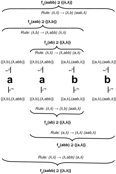
For example, suppose w=aabb. Figure 1 graphically gives the main steps of the computation of fG(aabb). Basically there are two ways to split aabb that allow the derivation of the empty context:
aab|b and a|abb. The first one corresponds to the top part of the figure while the second one is drawn at the bottom. We can see for instance that the empty context belongs to fG(ab)thanks to the
rule{(λ,λ)} → {(λ,abb)}{(a,λ)}:{(λ,abb)} ⊆fG(a)and{(a,λ)} ⊆ fG(b). But for symmetrical
reasons the result can also be obtained using the rule{(λ,λ)} → {(λ,b)}{(aab,λ)}.
As we trivially have fG(aa) = fG(bb) =/0, since no right-hand side contains the concatenation
of the same two features, an induction proof can be written to show that(λ,λ)∈ fG(w)⇔w∈ {anbn: n>0}.
Figure 1: The two derivations to obtain(λ,λ)in fG(aabb)in the grammar G.
We stop here the presentation of the CBFG formalism and we present our learning algorithm in the next section. However, if the reader wishes to become more familiar with CBFGs a study on their expressiveness is provided in Section 6.
4. Learning Algorithm
We have carefully defined the representation so that the inference algorithm will be almost trivial. Given a set of strings, and a set of contexts, we can simply write down a CBFG that will approximate a particular language.
4.1 Building CBFGs from Sets of Strings and Contexts
Definition 11 Let L be a language, F be a finite set of contexts such that(λ,λ)∈F, K a finite set of strings, PL={FL(u)→u|u∈K∧ |u|=1}and P={FL(uv)→FL(u)FL(v)|u,v,uv∈K}. We define
G0(K,L,F)as the CBFGhF,P,PL,Σi.
We will call K here the basis for the language. The set of productions is defined merely by observation: we take the set of all productions that we observe as the concatenation of elements of the small set K.
Let us explain the construction in more detail. PLis the set of lexical productions—analogous to
rules of the form N→a in a CFG in Chomsky normal form. These rules just assign to the terminal symbols their observed distribution—this will obviously be correct in that fG(a) =FL(a). P is the
interesting set of productions: these allow us to predict the features of a string uv from the features of its part u and v. To construct P we take all triples of strings u,v,uv that are in our finite set K. We observe that u has the contexts FL(u)and v has the set of contexts FL(v): our rule then states that
we can combine any string that has all of the contexts in FL(u)together with any string that has the
contexts in FL(v)and the result will have all of the contexts in FL(uv).
We will now look at a simple example. Let L={anbn |n>0}, F, the set of features is
{(λ,λ),(a,λ),(λ,b)} and K, the basis, is {a,b,ab,aa,aab}. For each of the elements of K we can compute the set of features that it has:
• FL(a)is just{(λ,b)}—this is the only one of the three contexts in F such that f⊙a∈L,
• FL(b) ={(a,λ)},
• FL(aa) = /0,
• FL(ab) ={(λ,λ)},
• FL(aab) ={(λ,b)}.
G0will therefore have the following lexical productions PL={(λ,b)} →a, {(a,λ)} →b. We
can now consider the productions in P. Looking at K we will see that there are only four possible triples of strings of the form uv,u,v: these are(aa,a,a),(ab,a,b),(aab,aa,b)and(aab,a,ab). Each of these will give rise to an element of P:
• The rule given by ab=a◦b:{(λ,λ)} → {(λ,b)}{(a,λ)},
• aa=a◦a gives /0 → {(λ,b)}{(λ,b)},
• aab=aa◦b gives{(λ,b)} → /0{(a,λ)},
• aab=a◦ab gives{(λ,b)} → {(λ,b)}{(λ,λ)}.
Given K,F and an oracle for L we can thus simply write down a CBFG. However, in this case, the language L(G0) is not the same as L; moreover, the resulting grammar is not exact.
Applying the rules for the recursive computation of fG, we can see that fG0(aab) ={(λ,b)}and
fG0(abb) = fG0(aabb) ={(λ,b),(λ,λ)}but FL(G0)(abb) ={(a,λ),(λ,b),(λ,λ)}and thus G0is not
exact. The problem here is caused by the fact that the production{(λ,b)} → /0{(a,λ)}allows any string to occur in the place specified by the /0: indeed since /0⊆ fG0(aab)and{(a,λ)} ⊆fG0(b)the
rule holds for aabb and thus{(λ,b)} ⊆ fG0(aabb). This is actually caused by the fact that there are
no contexts in F that correspond to the string aa in K.
a CBFG with almost no computation, but we still have the problem of finding suitable K and F—it might be that searching for exactly the right combination of K and F is intractably hard. It turns out that it is also very easy to find suitable sets.
In the next section we will establish two important lemmas that show that the search for K and F is fundamentally tractable: first, that as K increases the language defined by G0(K,L,F) will
increase, and secondly that as F increases the language will decrease.
Let us consider one example that illustrates these properties. Consider the language L={anb|
n≥0} ∪ {bam|m≥0} ∪ {a}.
First, let K={a,b,ab}and F={(λ,λ)}; then, by the definition of G0, we have the following
productions:
• {(λ,λ)} →a,
• {(λ,λ)} →b,
• {(λ,λ)} → {(λ,λ)}{(λ,λ)}.
It is easy to see that L(G0) =Σ+.
Now, suppose that F ={(λ,λ),(λ,b)}with K unchanged; then, by construction G0 will have
the following productions:
• {(λ,λ),(λ,b)} →a,
• {(λ,λ)} →b,
• {(λ,λ)} → {(λ,λ),(λ,b)}{(λ,λ)}.
The language defined by G0contains anb and also ansince{(λ,λ)} ⊂ {(λ,λ),(λ,b)}allowing the
third production to accept strings ending with an a. Thus, the language has been reduced such that L(G0) ={anb|n≥0} ∪ {am|m≥0}.
We continue by leaving F ={(λ,λ),(λ,b)}and we enlarge K such that K={a,b,ab,ba}. The productions in G0are:
• {(λ,λ),(λ,b)} →a,
• {(λ,λ)} →b,
• {(λ,λ)} → {(λ,λ),(λ,b)}{(λ,λ)}; the rule given by ab=a◦b,
• {(λ,λ)} → {(λ,λ)}{(λ,λ),(λ,b)}; the rule given by ba=b◦a.
The addition of the last rule allows the grammar to recognize ban and it can be easily shown that by a combination of the last two productions anbam belongs to the language defined by the grammar. Then, L(G0)has been increased such that L(G0) ={anbak|n,k≥0} ∪ {am|m≥0}.
In this example, the addition of(λ,b),(a,λ)and(λ,a)to F and the addition of aab and baa to K will then define the correct language. In fact this illustrates one principle of our approach: in the infinite data limit, the construction G0will define the correct language. In the following lemma we
abuse notation and use G0for when we have infinite K, and F: in this lemma we let K be the set of
Lemma 12 For any language L, let G=G0(Σ+,L,Σ∗×Σ∗). Then for all w∈Σ+ fG(w) =CL(w)
and therefore L(G) =L.
Proof By induction on the length of w. If |w|=1, and w=a then there is a lexical production CL(a)→a and by the definition of fG(a) =CL(a). Suppose this is true for all w with |w| ≤k.
Let w be some string of length k+1. Consider any split of w into u,v such that w=uv. fG(w)
is the union over all these splits of a function. We will show that every such split will give the same result of CL(w). By inductive hypothesis fG(u) =CL(u),fG(v) =CL(v). Since u,v,w are in
K =Σ+ we will also have an element of P of the form C
L(w)→CL(u)CL(v), so we know that
fG(w)⊇FL(w). We now show that fG will not predict any extra contexts. Consider every
pro-duction in P, FL(u′v′)→FL(u′)FL(v′), that applies to u,v, that is, with FL(u′)⊆fG(u) =CL(u)and
FL(v′)⊆ fG(v) =CL(v). Lemma 5 shows that in this case FL(u′v′)⊆FL(w)and thus we deduce that
fG(w)⊆FL(w), which establishes the lemma.
Informally if we take K to be every string and F to be every context, then we can accurately define any language. Of course, we are just interested in those cases where this can be defined finitely and we have a CBFG, in which case L will be decidable, but this infinite limit is a good check that the construction is sound.
4.2 Monotonicity Lemmas
We now prove two lemmas that show that the size of the language, and more particularly the features predicted will increase or decrease monotonically as a function of the basis K, and the feature set F, respectively. In fact, they give also a framework for approaching a target language from K and F.
Lemma 13 Suppose we have two CBFGs defined by G=G0(K,L,F)and G′=G0(K,L,F′)where
F⊆F′. Then for all u, fG(u)⊇ fG′(u)∩F.
Proof Let G′ have a set of productions P′,PL′, and G have a set of productions P,PL. Clearly if
x→yz∈P′then x∩F→(y∩F)(z∩F)is in P by the definition of G0, and likewise for PL,PL′. By
induction on|u|we can show that any feature in fG′(u)∩F will be in fG(u). The base case is trivial since FL′(a)∩F=FL(a); if it is true for all strings up to length k, then if f ∈ fG′(u)∩F; there must be a production in F′ with f on the head. By the inductive hypothesis, the right hand sides of the corresponding production in P will be triggered, and so f must be in fG(u).
Corollary 14 Suppose we have two CBFGs defined by G=G0(K,L,F) and G′ =G0(K,L,F′)
where F⊆F′; then L(G)⊇L(G′).
Proof It is sufficient to remark that if u∈L(G′)then(λ,λ)∈ fG′(u)⊆fG(u)and thus u∈L(G).
Conversely, we can show that as we increase K, the language and the map fGwill increase. This
is addressed by the next lemma.
Lemma 15 Suppose we have two CBFGs defined by G=G0(K,L,F)and G′=G0(K′,L,F)where
Proof Clearly the sets of productions of G0(K,L,F)will be a subset of the set of productions of G0(K′,L,F), and so anything that can be derived by the first can be derived by the second, again by
induction on the length of the string.
A simple result is that when K contains all of the substrings of a word, then G0(K,L,F) will
generate all of the correct features for this word.
Lemma 16 For any string w, if Sub(w)⊂K, and let G=G0(K,L,F), then FL(w)⊆ fG(w). Proof By recursion on the size of w. Let G=G0(K,L,F) =hF,P,PL,Σi. First, notice that if w is of
length 1 then we have FL(w)→w in PLand thus the lemma holds. Then suppose that|w|=k≥2.
Let u and v in Σ+ be such that w=uv. As Sub(w)⊂K we have u,v in K. Therefore the rule FL(w)→FL(u)FL(v)belongs to P. As|u|<|w|and|v|<|w|, by recursion we get FL(u)⊆ fG(u)
and FL(v)⊆ fG(v). Thus the rule can be applied and then FL(w)⊆ fG(w).
In particular if w∈L, and Sub(w)⊆K, then w∈L(G). This means that we can easily increase the language defined by G just by adding Sub(w)to K. In general we do not need to add every element of Sub(w)—it is enough to have one binary bracketing.
To establish learnability, we need to prove that for a target language L, if we have a sufficiently large F then L(G0(K,L,F))will be contained within L and that if we have a sufficiently large K,
then L(G0(K,L,F))will contain L.
4.3 Fiducial Feature Sets and Finite Context Property
We need to be able to prove that for any K if we have enough features then the language defined will be included within the target language L. We formalise the idea of having enough features in the following way:
Definition 17 For a language L and a string u, a set of features F is fiducial on u if for all v∈Σ∗, FL(u)⊆FL(v)implies CL(u)⊆CL(v).
Note that if F is fiducial on u and F⊂F′ then F′is fiducial on u. Therefore we can naturally extend this to sets of strings.
Definition 18 For a language L and a set of strings K, a set of features F is fiducial on K if for all
u∈K, F is fiducial on u.
Clearly, for any string w, CL(w) will be fiducial on w; but this is vacuous—we are interested
in cases where there is a finite set of contexts which is fiducial for w, but where CL(w) is infinite.
If u and v are both in K then having the same features means they are syntactically congruent. However if two strings, neither of which are in K, have the same features this does not mean they are necessarily congruent (for instance if FL(v) =FL(v′) = /0). For non finite state languages, the set
Let us consider our running example L={anbn|n>0}. Take the string ab. CL(ab)is infinite and
contains contexts of the form(λ,λ),(a,b),(aa,bb)and so on. Consider a set with just one of these contexts, say F={(a,b)}. This set is clearly fiducial for ab, since the only strings that will have this context are those that are congruent to ab. Consider now the string aab; clearly{(λ,b)}is fiducial for aab, even though the string a, which is not congruent to aab also occurs in this context. Indeed, this does not violate fiduciality since CL(a)⊃CL(aab). However, looking at string a,{(λ,b)}is not
fiducial, since aab has this context but does not include all the contexts of a such as, for example,
(λ,abb).
In these trivial examples, a context set of cardinality one is sufficient to be fiducial, but this is not the case in general. Consider the finite language L={ab,ac,db,ec,dx,ey}, and the string a. It has two contexts(λ,b)and(λ,c)neither of which is fiducial for a on its own. However, the set of both contexts is:{(λ,b),(λ,c)}is fiducial for a.
We now define the finite context property, which is one of the two conditions that languages must satisfy to be learnable in this model; this condition is a purely language theoretic property.
Definition 19 A language L has the Finite Context Property (FCP) if every string has a finite
fidu-cial feature set.
Clearly if L has the FCP, then any finite set of substrings, K, has a finite fiducial feature set which will be the union of the finite fiducial feature sets for each element of K. If u6∈Sub(L)then any set of features is fiducial since CL(u) =/0.
We note here that all regular languages have the FCP. We refer the reader to the Section 6.1.1 about CBFG and regular languages where the Lemma 35 and the associated construction proves this claim.
We can now state the most important lemma: this lemma links up the definition of the feature map in a CBFG, with the fiducial set of features to show that only correct features will be assigned to substrings by the grammar. It states that the features assigned by the grammar will correspond to the language theoretic interpretation of them as contexts.
Lemma 20 For any language L, given a set of strings K and a set of features F, let G=G0(K,L,F).
If F is fiducial on K, then for all w∈Σ∗ f
G(w)⊆FL(w).
Proof We proceed by induction on length of the string. Base case: strings of length 1. fG(w)will
be the set of observed contexts of w, and since we have observed these contexts, they must be in the language. Inductive step: let w a string of length k.
Take a feature f on fG(w); by definition this must come from some production x→yz and a split
u,v of w. The production must be from some elements of K, u′,v′and u′v′such that y=FL(u′),z=
FL(v′)and x=FL(u′v′). If the production applies this means that FL(u′) =y⊆fG(u)⊆FL(u)(by
in-ductive hypothesis), and similarly FL(v′)⊆FL(v). By fiduciality of F this means that C(u′)⊆C(u)
and C(v′)⊆C(v). So by Lemma 5 C(u′v′)⊆C(uv). Since f ∈C(u′v′) then f ∈C(uv) =C(w). Therefore, since f ∈F and C(w)∩F=FL(w), f ∈FL(w), and therefore fG(w)⊆FL(w).
Corollary 21 If F is fiducial on K then L(G0(K,F,L))⊆L.
4.4 Kernel and Finite Kernel Property
We will now show a complementary result, namely that for a sufficiently large K the language defined by G0will include the target language. We will start by formalising the idea that a set K is
large enough, by defining the idea of a kernel.
Definition 22 A finite set K ⊆Σ∗ is a kernel for a language L, if for any set of features F,
L(G0(K,F,L))⊇L.
Consider again the language L={anbn|n≥0}. The set K={a,b,ab}is not a kernel, since if we have a large enough set of features, then the language defined will only be{ab} which is a proper subset of L. However K={a,b,ab,aab,abb,aabb}is a kernel: no matter how large a set of features we have the language defined will always include L. Consider a language L′=L∪ {b16}. In this case, a kernel for L′must include, as well as a kernel for L, some set of substrings of b16: it is enough to have b16,b8,b4,bb,b.
To prove that a set is a kernel, it suffices to show that if we consider all the possible features for building the grammar, we will contain the target language; any smaller set of features defines then a larger language. In our case, we can take the infinite set of all contexts and define productions based on the congruence classes. If F is the set of all contexts then we have FL(u) =CL(u), thus the
productions will be exactly of the form C(uv)→C(u)C(v). This is a slight abuse of notation since feature sets are normally finite.
Lemma 23 Let F=Σ∗×Σ∗; if L(G0(K,L,F))⊇L then K is a kernel. Proof By monotonicity of F: any finite feature set will be a subset of F.
Not all context-free languages will have a finite kernel. For example L={a+} ∪ {anbm|n<m}
is clearly context-free, but does not have a finite kernel. Assume that the set K contains all strings of length less than or equal to k. Assume w.l.o.g. that the fiducial set of features for K includes all features(λ,bi), where i≤k+1. Consider the rules of the form FL(ak)→FL(aj)FL(ak−j); we can
see that no matter how large k is, the derived CBFG will undergenerate as ak is not congruent to ak−1.
Definition 24 A context-free grammar GT =hV,S,P,Σi has the Finite Kernel Property (FKP) iff
for every non-terminal N∈V there is a finite set of strings K(N)such that a∈K(N)if a∈Σand N→a∈P and such that for all k∈K(N),N⇒∗ k and where for every string w∈Σ∗such that N⇒∗ w there is a string k∈K(N)such that C(k)⊆C(w). A CFL L has the FKP, if there is a grammar in CNF for it with the FKP.
Notice that all regular languages have the FKP since they have a finite number of congruence classes.
Lemma 25 Any context-free language with the FKP has a finite kernel. Proof Let GT=hV,S,P,Σibe such a CNF CFG with the FKP. Define
K(GT) = [
N∈V
K(N)∪ [ X→MN∈P
K(M)K(N)
!
We claim that K(GT) is a kernel. Assume that F =Σ∗×Σ∗ and let G be such that G=
G0(K(GT),L(GT),F) =hF,(λ,λ),P,PL,Σi.
We will show, by induction on the length of derivation of w in GT, that for all N,w if N⇒∗ w
then there is a k in K(N) such that fG(w)⊇C(k). If length of derivation is 1, then this is true
since|w|=1 and thus w∈K(N): therefore C(w)→w∈PL. Suppose it is true for all derivations
of length less than j. Take a derivation of length j; say N ⇒∗ w. There must be a production in GT of the form N→PQ, where P⇒∗u and Q⇒∗ v, and w=uv. By inductive hypothesis; we
have fG(u)⊇C(ku) and fG(v)⊇C(kv). By construction kukv∈K(GT) and then there will be a
rule C(kukv)→C(ku)C(kv)in P. Therefore fG(uv)⊇C(kukv). Since N ∗
⇒kukv there must be some
kuv∈K(N)such that C(kuv)⊆C(kukv). Therefore fG(w)⊇C(kukv)⊇C(kuv).
Now we can see that if w∈L, then S⇒∗ w, then there is a k∈K(S)such that fG(w)⊇C(k)and
S⇒∗ k, therefore(λ,λ)∈ fG(w)since(λ,λ)∈C(k), thus w∈L(G)and therefore K is a kernel.
4.5 Learning Algorithm
Before we present the algorithm, we will discuss the learning model that we use. The class of languages that we will learn is suprafinite and thus we cannot get a positive data only identifica-tion in the limit result (Gold, 1967). Ultimately we are interested in a more realistic probabilistic learning paradigm, but for mathematical convenience it is appropriate to establish the basic results in a symbolic paradigm. The ultimate goal is to model natural languages, where negative data, or equivalence queries are generally not available or are computationally impossible. Accordingly, we have decided to use the model of positive data together with membership queries: an oracle can tell the learner whether a string is in the language or not (Angluin, 1988). The presented algorithm runs in time polynomial in the size of the sample S: since the strings are of variable length, this size must be the sum of the lengths of the strings in S,kSk=∑w∈S|w|. We should note that this is not a strong enough result: Pitt (1989) showed that any algorithm can be made polynomial, by only processing a small prefix of the data. It is hard to tighten the model sufficiently: the suggestion of de la Higuera (1997) for a polynomial characteristic set is inapplicable for representations, such as the ones in this paper, that are powerful enough to define languages whose shortest strings are exponentially long. Accordingly we do not require in this model a polynomial dependence on the size of the represen-tation. We note that the situation is unsatisfactory, but we do not intend to propose a solution in this paper. We merely point out that the algorithm is genuinely polynomial and processes all of the data in the sample without “delaying tricks” of the type discussed by Pitt.
Definition 26 A class of languages L is identifiable in the limit (IIL) from positive data and a membership oracle with polynomial time and queries iff there exist two polynomials p(),q()and an algorithm A such that:
• Given an infinite presentation of positive examples S, where Sn is the first n examples of the
presentation,
1. A returns a representation G=A(Sn)in time p(kSnk).
2. A asks at most q(kSnk)queries to build A(Sn).
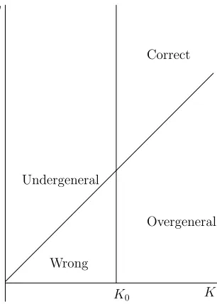
K F
K0
Overgeneral Correct
Undergeneral
Wrong
Figure 2: The relationship between K and F: The diagonal line is the line of fiduciality: above this line means that F is fiducial on K. K0is a kernel for the language.
Before we present the algorithm we hope that it is intuitively obvious how the approach will work. Figure 2 diagrammatically shows the relationship between K and F. When we have a large enough K, we will be to the right of the vertical line; when we have enough features for that K we will be above the diagonal line. Thus the basis of the algorithm is to move to the right, until we have enough data, and then to move up vertically, increasing the feature set until we have a fiducial set.
We can now define our learning algorithm in Algorithm 1. Informally, D is the list of all strings that have been seen so far and Gnis the current grammar obtained with the first n strings of D. The
algorithm uses two tests: one test is just to determine if the current hypothesis undergeneralises. This is trivial, since we have a positive presentation of the data, and so eventually we will be presented with a string in L\L(Gn). In this case we need to increase K; we accordingly increase K to the set
of all substrings that we have observed so far. The second test is a bit more delicate. We want to detect if our algorithm overgeneralises. This requires us to search through a polynomially bounded set of strings looking for a string that is in L(Gn)\L. An obvious candidate set is Con(D)⊙Sub(D);
but though we conjecture that this is adequate, we have not yet been able to prove that is correct, as it might be that the overgenerated string does not lie in Con(L)⊙Sub(L).
Here we use a slightly stricter criterion: we try to detect whether F is fiducial for K: we search through a polynomially bounded set of strings, Sub(D), to find a violation of the fiduciality condi-tion. If we find such a violation, then we know that F is not fiducial for K, and so we increase F to the set of all contexts that we have seen so far, Con(D).
In Algorithm 1, G0(K,
O
,F)denotes the same construction as G0(K,L,F), except that we usemembership queries with the oracle
O
to compute FLfor each element in K. We give theAlgorithm 1: CBFG learning algorithm IIL
Data: A sequence of strings S={w1,w2. . . ,}, membership oracle
O
Result: A sequence of CBFGs G1,G2, . . .K← /0; D← /0; F← {(λ,λ)}; G=G0(K,
O
,F); for widoD←D∪ {wi}; C←Con(D); S←Sub(D); if ∃w∈D\L(G)then
K←S ; F←C ;
end
else if∃v∈S,u∈K,f ∈C such that FL(u)⊆FL(v)and f⊙u∈L but f⊙v6∈L then
F←C ;
end
G=G0(K,
O
,F);Output Gi=G ; end
Theorem 27 Algorithm 1 runs in polynomial time in the size of the sample, and makes a polynomial
number of calls to the membership oracle.
Proof The value of D will just be the set of observed strings; Sub(D)and Con(D)are both polyno-mially bounded by the size of the sample, and therefore so are|K|and|F|. Therefore the number of calls to the oracle is clearly polynomial, as it is bouned by|K||F|. Computing G0is also polynomial,
since|P| ≤ |K|2, and all strings involved are in Sub(D).
4.6 Identification in the Limit Result
In the following, we consider the class of context-free languages having the FCP and the FKP, represented by CBFG. Kndenotes the value of K at the nthloop, and similarly for F, D.
Definition 28
L
CFGis the class of all context-free languages that satisfy the FCP and the FKP.In what follows we assume that L is an element of this class, and that w1, . . . ,wn, . . .is a infinite
presentation of the language. The proof is straightforward and merely requires an analysis of a few cases. We will proceed as follows: there are 4 states that the model can be in, that correspond to the four regions of the diagram in Figure 2.
1. K is a kernel and F is fiducial for K; in this case the model has converged to the correct answer. This is the region labeled correct in Figure 2.
2. K is a kernel and F is not fiducial for K: then L⊆L(G), and at some later point, we will increase F to a fiducial set, and we will be in state 1: this is the region labeled overgeneral.
4. K is not a kernel and F is not fiducial: in this case at some point we will move to states 1 or 2. This is the area labeled wrong.
We will start by making some basic statements about properties of the algorithm:
Lemma 29 If there is some n, such that Fnis fiducial for Knand L(Gn) =L, then the algorithm will
not change its hypothesis: that is, for all n>N, Kn=KN,Fn=FNand therefore Gn=GN.
Proof If L(Gn)is correct, then the first condition of the loop will never be met; if Fnis fiducial for
Kn, then the second condition will never be satisfied.
Lemma 30 If there is some N such that KN is a kernel, then for all n>N, Kn=KN.
Proof Immediate by definition of a kernel, and of the algorithm.
We now prove that if F is not fiducial then the algorithm will be able to detect this.
Lemma 31 If there is some n such that Fnis not fiducial for Kn, then there is some index n′≥n at
which Fnwill be increased.
Proof If Fnis not fiducial, then by definition there is some u∈K, v∈Σ+such that FL(u)⊆FL(v),
but there is an f ∈CL(u)that is not in CL(v). By construction FL(u)is always non-empty, and so
is FL(v). Thus v∈Sub(L). Note f⊙u∈L, so f ∈Con(L). Let n′be the smallest index such that
v∈Sub(Dn)and f ∈Con(Dn): at this point, either Fn will have changed, or not, in which case it
will be increased at this point.
We now prove that we will always get a fiducial feature set.
Lemma 32 For any n, there is some n′such that Fn′ is fiducial for Kn.
Proof If Fnis fiducial then n′=n satisfies the condition. Assume otherwise. Let F be a finite set
of contexts that is fiducial for Kn. We can assume that F⊆Con(L). Let n1be the first index such
that Con(Dn1)contains F. At this point we are not sure that Fn1 =Con(Dn1)since the conditions
for changing the set of contexts may not be reached. Anyhow, if it is the case then Fn1 is fiducial,
then n1=n′ satisfies the condition. If not, then by the preceding lemma, there must be some point
n2 at which we will increase the set of contexts of the current grammar; Fn2 =Con(n2)must
con-tain F since Con(Dn1)⊂Con(Dn2), and is therefore fiducial, and so n2=n
′satisfies the condition.
Lemma 33 For every positive presentation of an L∈
L
CFG, there is some n such that either theProof Let m be the smallest number such that Sub(Dm) is a kernel. Recall that any superset of a
kernel is a kernel, and that all CFL with the FKP have a finite kernel (Lemma 25), and that such a kernel is a subset of Sub(L), so such an m must exist.
Consider the grammar Gm; there are three possibilities:
1. L(Gm) =L, and Fmis fiducial, in which case the grammar has converged.
2. L(Gm) is a proper subset of L and Fm is fiducial. Let m′ be the first point at which wm′ is in L\L(Gm); at this point Km′ will be increased to include Sub(Dm)and it will therefore be a kernel. 3. Fmis not fiducial: in this case by Lemma 32; there is some n at which Fnis fiducial for Km. Either
Kn=Kmin which case this reduces to Case 2; or Knis larger than Kmin which case it must be a
kernel, since it will include Sub(Dm)which is a kernel.
We now can prove the main result of the paper:
Theorem 34 Algorithm 1 identifies in the limit the class of context-free languages with the finite
context property and the finite kernel property.
Proof By Lemma 33 there is some point at which it converges or has a kernel. If Knis a kernel then
by Lemma 32, there is some point n′ at which we have a fiducial feature set. Therefore L(Gn′) =L, and the algorithm has converged.
4.7 Examples
We will now give a worked example of the algorithm. Suppose L={anbn|n>0}.
G0 will be the empty grammar, with K = /0,F ={(λ,λ)} and an empty set of productions.
L(G0) =/0.
1. Suppose w1=ab. D={ab}. This is not in L(G0)so we set • K=Sub(D) ={a,b,ab}.
• F=Con(D) ={(λ,λ),(a,λ),(λ,b)}.
This gives us one production: FL(ab) → FL(a)FL(b) which corresponds to {(λ,λ)} → {(λ,b)}{(a,λ)}, and the lexical productions{(λ,b)} →a,{(a,λ)} →b. The language de-fined is thus L(G1) ={ab}.
2. Suppose w2=aabb. D={ab,aabb}. This is not in L(G1)so we set • K=Sub(D) ={a,b,ab,aa,bb,aab,abb,aabb}.
• F=Con(D) ={(λ,λ),(a,λ),(λ,b),(aa,λ),(a,b),(λ,bb),(aab,λ),(aa,b),
(a,bb),(λ,abb)}.
• FL(ab)→FL(a),FL(b)which is
{(λ,λ),(a,b)} → {(a,bb),(λ,abb),(λ,b)},{(aa,b),(aab,λ),(a,λ)}.
• FL(aab)→FL(a),FL(ab)which is
{(a,bb),(λ,b)} → {(a,bb),(λ,abb),(λ,b)},{(λ,λ),(a,b)}.
• FL(aab)→FL(aa),FL(b)which is
{(a,bb),(λ,b)} → {(λ,bb)},{(aa,b),(aab,λ),(a,λ)}.
• FL(bb)→FL(b),FL(b)which is
{(aa,λ)} → {(aa,b),(aab,λ),(a,λ)},{(aa,b),(aab,λ),(a,λ)}.
• FL(aa)→FL(a),FL(a)which is
{(λ,bb)} → {(a,bb),(λ,abb),(λ,b)},{(a,bb),(λ,abb),(λ,b)}.
• FL(aabb)→FL(a),FL(abb)which is
{(λ,λ),(a,b)} → {(a,bb),(λ,abb),(λ,b)},{(aa,b),(a,λ)}.
• FL(aabb)→FL(aa),FL(bb)which is
{(λ,λ),(a,b)} → {(λ,bb)},{(aa,λ)}.
• FL(aabb)→FL(aab),FL(b)which is
{(λ,λ),(a,b)} → {(a,bb),(λ,b)},{(aa,b),(aab,λ),(a,λ)}.
• FL(abb)→FL(a),FL(bb)which is
{(aa,b),(a,λ)} → {(a,bb),(λ,abb),(λ,b)},{(aa,λ)}.
• FL(abb)→FL(ab),FL(b)which is
{(aa,b),(a,λ)} → {(λ,λ),(a,b)},{(aa,b),(aab,λ),(a,λ)}.
and the two lexical productions:
• FL(a)→a which is{(a,bb),(λ,abb),(λ,b)} →a • FL(b)→b which is{(aa,b),(aab,λ),(a,λ)} →b.
K is now a kernel and L(G) =L, but F is not fiducial for K, since(λ,bb)is not fiducial for aa (consider aaab).
3. Suppose w3=aaabbb. Now |Con(D3)|=21; there are now several elements of Con(D3)
that are similar. For example(λ,λ),(a,b)and(aa,bb)are identical but as it is harmless for the resulting grammar, it does not mind. Now we will detect that F is not fiducial: we will find v=aaab, u=aa and f = (λ,abbb); FL(aa) ={(λ,bb)}=FL(aaab), but f⊙aaab=
aaababbb which is not in L. We will therefore increase F to be Con(D3), and then the
5. Practical Behavior of the Algorithm
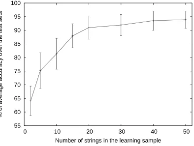
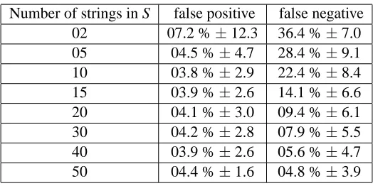
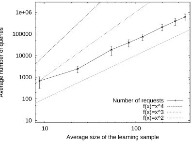
In this section, we propose to study the behavior of our algorithm from a practical point of view. We focus more specifically on two important issues. The first one deals with the learning ability of the algorithm when the conditions for the theoretical learning result are not reached. Indeed, although the identification in the limit paradigm proves that with sufficient data it is possible to obtain exact convergence, it says nothing about the convergence when fewer learning examples are available: does the output get closer and closer to the target until it reaches it or does it stay far from the expected solution until receives enough data? The second question concerns the learning behavior of the algorithm: does it tend to over-generalise or to under-generalise?
For our experimental setup, we need to select appropriate data sets. In grammatical inference little has been done concerning benchmarking. The main available corpora are those of the on line competitions organised by the International Colloquium on Grammatical Inference. Three different competitions have recently taken place: the Abbadingo One (Lang et al., 1998) which was about regular languages, the Omphalos competition on context-free languages (Starkie et al., 2004) and the Tenjino competition (Starkie et al., 2006) dealing with transducers learning. Note that some of these data sets correspond to extremely hard learning problems since their main objective was to push the state of the art (some problems of the Abbadingo One competition are still unsolved more than ten years after its official end!)
However, these data sets can not be directly used for evaluating our algorithm because the solutions or the target models are not available. Our algorithm needs an oracle and thus we need a way to give answers to membership queries. In order to overcome this drawback, we chose to build synthetically some data sets following the experimental setup proposed by these competitions. More precisely, we decided to randomly generate target context-free grammars following what has been done for the Omphalos competition. Each grammar is then used either to generate training and test sets or as an oracle for answering membership queries.
In the following paragraphs we describe first the generation of the target context-free gram-mars, then the experimental setup with learning and test data sets used and finally the results and conclusions that can be drawn.
5.1 Generation of Target Context-free Grammars
The main difference with the Omphalos generation process is that we do not especially need non-regular languages. Indeed, one of the aim of these experiments is to give an idea on the behavior of the algorithm when its theoretical assumptions are not likely to be valid. From this standpoint, all randomly generated non-finite languages are good candidates as learning targets. However, with a similar principle used for the Omphalos competition, we checked that some of the generated grammars can not be easily solved by methods for regular languages. Although we can not decide if these grammars define non regular context-free languages, it ensures us that the target models are at least not too simple.
5.2 Experimental Setup
For each target grammar we generate a learning and a test sample following the Omphalos com-petition requirements. We build the learning sample by first creating a structurally complete set of strings for each grammar. This set is built such that for each rule of the target grammar, at least one string of the set can be derived using this rule (Parekh and Honavar, 1996). This would guarantee that the complete learning set would have the minimal amount of information for finding the struc-ture of the grammar. We then complete this learning set by randomly generating new strings from the grammar in order to have a total of 50 examples. We chose arbitrarily this value for two reasons: first it is sufficient to ensure that each sample strictly contains a structurally complete set for each target grammar and secondly we are likely to be far from the guarantees of the identification in the limit framework.
The construction of the test set needs particular attention. Since the learning phase uses a mem-bership oracle, when the hypothesis is being constructed, some new strings may be built and queried for the oracle by picking a substring and a context from the learning sample. Thus, even if the test set does not contain any string of the learning sample, the construction G0may consider some strings
present in the test set. In order to avoid this drawback, that is, to guarantee that no string of the test could be seen during the construction of the CBFG, each test string has a length of at least 3 times the maximal length of the strings in the learning set, which is by construction the maximal size of the strings queried. According to this procedure, we randomly generate a test set of 1000 strings over the alphabet of terminal symbols used to define the target grammar (1000 examples is twice the size of the small test sets of the Omphalos competition). The test sequences are then labeled positive or negative depending on their membership to the language defined by the grammar. We repeat this process until we have the desired number of strings. The ratio between strings in the language and strings outside the language is fixed to be between 40% and 60%.
In order to study the behavior of our algorithm, we define the following setup. For each target context-free grammar, we construct a CBFG by applying the construction G0(K,
O
,F) with K=Sub(S)and F=Con(S)where S is a set of strings drawn from the learning set and using the target grammar as the oracle