Tracking Methods to Study the Surface Regression of the
Solid-Propellant Grain
Yao Hsin Hwang
1and Chung Hua Chiang
2, *1Department of Marine Engineering, National Kaohsiung Marine University, Kaohsiung, Taiwan. 2Department of Mechanical and Automation Engineering, I-Shou University, Kaohsiung, Taiwan.
Received 08 April 2014; received in revised form 22 April 2014; accepted 30 May 2014
Abstract
In the work, we have successfully developed practical surface tracking methods to calculate the erosive
volume and the associated burning areas which are the important parameters to solve a nonlinear,
pressurization-rate dependent combustion ballistics. Three methodologies, namely the front tracking, the
emanating ray and the least distance methods, are proposed. The front tracking method is based on the
Lagrangian point of view; while both the emanating ray and the least distance methods are formulated from the
Eulerian viewpoint. Two two-dimensional test problems have been examined to compare with the programming
complexity, simulation accuracy and required CPU time of the proposed methods. It is found that the least
distance method performs superior to the other two methods in numerical respects. The least distance method is
implemented with tetrahedron grids to track the outward propagation of a three-dimensional cubic.
Comparison between the predicted erosive volume and corresponding theoretical result yields satisfactory
agreement.
Keywords: solid propellant surface regression, surface tracking methods, CFD
1.
Introduction
The tremendous complexity of solid propellant rocket systems has received almost universal and tacit recognition.
However, the basic idea behind a solid-propellant rocket motor is simple: thrust arises from pressurization of a vented
chamber by mass injection which is caused by the burning of the propellant. Its detailed behavior is quite complicated
because the combustion rate depends on the chamber pressure as well as the propellant’s surface area, storage temperature,
and composition. For the readers may unfamiliar with the theoretical state-of-the-art in propellant combustion, the
fundamental study can be found in [1] and the compilation of expert articles in [2] is a valuable resource.
In general, the rocket motor’s operation and design depend heavily on the combustion characteristics of the propellant,
its burning rate, burning surface, storage temperature, and composition. The solid propellant’s shape, called the propellant
grain determines the burning surface area, which in turn affects how the thrust varies over time-progressive, regressive, or
neutral profiles are possible. Usually, the propellant grain is not just a simple cylinder, but often has slots and fins in its
interior cavity to increase the surface area. The propellant surface regresses as propellant is consumed, so the shape and area
of the burning surface change dynamically with time. The coupling and feedback between these variables can lead to
instabilities. These problems are characterized by very-high-energy densities; extremely diverse length and time scales;
dynamically changing geometries; complex interfaces; and reactive, turbulent, multiphase flows. Because of the complexity
*Corresponding author. E-mail address: [email protected]
of the components and their interactions, conventional rocket-design techniques have largely been limited to a relatively
simple lumped system modeling based on gross thermo-mechanical properties, and have relied heavily on experimental trial
and error. Simulation of each component is a challenging problem in its own right, both in terms of developing realistic
models and in the computational capacity required solving them accurately.
To coordinate the overall predictions of the interior ballistics of modern solid-propellant rocket motors and thruster gas
dynamics, combustion sub-models and simulation codes must be developed to calculate transient variation of pressure
distribution, velocity profile, burning rates, gas-phase combustion kinetics, and overall rocket thrust. To meet these
objectives, a numerical framework is proposed which permits the calculation of the pressure and thrust curve of a motor
supported by a homogeneous propellant, allowing for complete coupling between the condensed phase physics, the
gas-phase physics, and the unsteady, uneven, regressing surface. It would require developing a code to simulate the
propagation of a burning front in a solid propellant rocket model. The overall approach relies on a combination of interface
tracking method to capture the motion of the gas/solid interface and a gas-phase transient analysis of pressure. The integrated
code must be able to predict the grain surface regression rate and overall mass flow rate through the nozzle accurately. This
study will focus on the methods of surface tracking. The details will be described as follows.
2.
Numerical Methods for Surface Tracking of the Grain
The direct numerical simulation of solid-propellant grain burnout needs the solution of a moving boundary problem,
which for the present discussion is represented by the evolution of the three-dimensional solid grain shape. To carry out the
solution, one must choose an algorithm to represent the grain surface at any instant and to compute its motion. Various
numerical attempts exist in the literature to realize tracking interface [3]. In general there are two kinds of methods which
have been widely used for the surface tracking of grain regression, namely the front tracking method and the front capturing
method. The former is described by using a Larangian approach, while the latter is based on an Eulerian view. The most
commonly used method for tracking moving boundaries in a Larangian framework is the marker/string method or nodal
method [4]. The popular methods for tracking moving boundaries in an Eulerian framework are the volume-of-fluid method
and its refinements [5, 6], the level-set method [7, 8], and the phase-field method [9]. These methods perform very well in
problems involving free surfaces. For the particular problems of interest here, namely, tracking of solid–gas phase fronts, the
level-set method [10, 11], the phase-field method [12, 13], and enthalpy type methods [14, 15] have been employed. In these
purely Eulerian methods, the interface is not tracked explicitly but is deduced based on a field variable such as the distance
function, order parameter, or local enthalpy. The interface is of finite thickness and may occupy a few grid points in a
direction normal to it. Although these methods converge to the sharp interface models as the grid size has decreased,
numerical difficulties restrict operation of these methods because interface thicknesses is proportional to the grid size. Based
on above methodologies, many researchers or rocket companies have developed sophisticated internal ballistics code to deal
with fluid structure interactions with moving boundary [16-20]. However, for developing the own internal ballistics code,
some people may find out that the above methods are usually too complicated in math and difficult in topology to extend to a
three-dimensional calculation.
In the present work, we try to use different methodologies without involving too much math but with a simple physics
that is essential on the basic idea. Currently advanced internal ballistics models can deal with heterogeneous combustion
with the cost of handling complexities of surface tracking significantly. To make it simple, we assume the propellant
burning rate is isotropically homogeneous in the combustor. That is, the propellant erosive velocity is uniform in all
directions. It can be analog to the propagation of wave front of a point source. Therefore, the required burning distance at a
specific location will be the shortest one which originated from the initial burning surface, i.e. the normal distance from the
Copyright © TAETI distance. We test three proposed methods to estimate the burning volume of uniform solid propellants: front tracking, method
of emanating ray and least distance. More details are as follows.
2.1. Front tracking method
In the front tracking method, the currently burning segments are evolved into the unburned region by the velocity
according to the specified burning rate. Technical details may be paid to appropriately handle the entanglement, addition and
elimination of burning segments. The resulting algorithm can be summarized as follows:
(1) The initial surface is constructed as consecutive segments. Segments can be the line segments in the two-dimensional case and the surfaces in the three-dimensional case.
(2) Move the surface segments in its normal direction at a burn distance. If a convex corner is formed, there is a need to add the segments to form a circular arc based on the Huygens principle. If a concave corner is formed, the intersected segments can be resulted after the move. There is a need to delete the segment sections beyond the intersecting point.
(3) Connect the remaining segments to form the new surface segments.
(4) Treat the new segments as initial ones and return to step 2.
Obviously, this can be categorized as a Lagrangian method.
2.2. Emanating ray method
The methods of emanating rays and least distance require a background grid, which is arisen from the Eulerian point
of view. The actual burn distance for each node is recorded and the current burn surface is determined by the contour lines
for a given burn distance. The algorithm of emanating rays is:
(1) Construct non-overlapping cells in the interested region. The initial burn surface is constructed as consecutive segments.
(2) Emanate a ray from each initial segment in its normal direction and estimate the distance for all visited cells that this ray has passed through. If a convex corner is formed, emanate additional distance rays from each convex corner and estimate the distance for all visited cells.
(3) Assign the shortest distance as the resulting distance for a cell if it is visited by multiple rays.
The emanating rays must be sufficiently dense such as all constructed cell must be visited. The emanating direction
should be normal to the segment surface.
2.3. The least distance method
The detailed steps for the method of least distance can be itemized as follows:
(1) Construct non-overlapping cells in the interested region. The initial burn surface is constructed as consecutive segments.
(2) For each node of every cell, determine the distance from the node to each surface segment.
(3) Assign the shortest distance as the resulting distance for the node.
(4) The burning surface is located at the contour of each constant distance function.
The location at a surface to determine the shortest distance will be the perpendicular point on at surface, edge or both
end points. It can be easily checked with the computational geometry methods.
3.
Results and Discussions
The above three methods are tested by two numerical examples. Example 1 is to test the effect of discontinuity of
convex surface on the evolution process from an initial squared region. The resulting contour lines for above three methods
are shown in Figures 1, 2 and 3. It is observed that the sharp corner diminishes and an expansion fan is developed. The
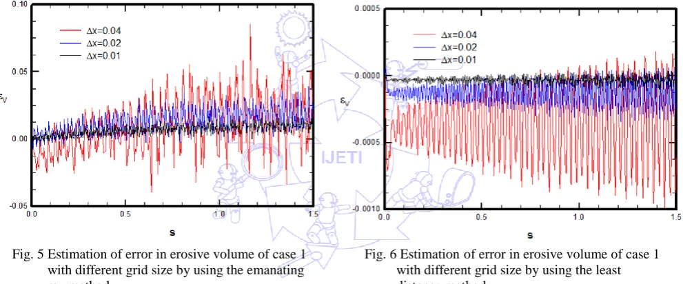
estimation errors of the erosive volume (ε_v) for these methods with different grid spacing are correspondingly shown in
methods with exact solution is presented in Figure 7. It is indicated that all these methods can yield quite satisfactory results
and close to the exact solution. We can see the error increasing progressively with the burn distance and the error increases as
the grid size increases for the front tracking method. The error seems independent on the burn distance but slightly depends
on grid size for the emanating ray method and for the least distance method.
Fig. 1 Contours of regressing surface by using the front tracking method
Fig. 2 Contours of regressing surface by using the emanating ray method
Copyright © TAETI Fig. 4 Estimation of error in erosive volume of case 1 with different grid sizes by using the front tracking method
Fig. 5 Estimation of error in erosive volume of case 1 with different grid size by using the emanating ray method
Fig. 6 Estimationof error in erosive volume of case 1 with different grid size by using the least distance method
The second test example is to investigate discontinuity of the concave surface for the evolution of an initial cross
shape. The resulting contours are presented in Figures 8, 9 and 10 for three different methods. The propagation of
discontinuity on concave surface usually develops a shock. In order to ensure that shock won’t stall the algorithm, care must
be taken to delete portions of intersecting segments when working with the front tracking method. The other two Eulerian
approach based methods do not suffer this kind of difficulty in coding the program. No shock-like compressed regions have
observed for all three methods. Comparison of erosive volume for three different methods is shown in Figure 11. Our
calculations indicated that all three methods yield almost have the same results.
Fig. 8 Evolution of an initial cross shape by using the front tracking method
Fig. 9 Evolution of an initial cross shape by using the emanating ray method
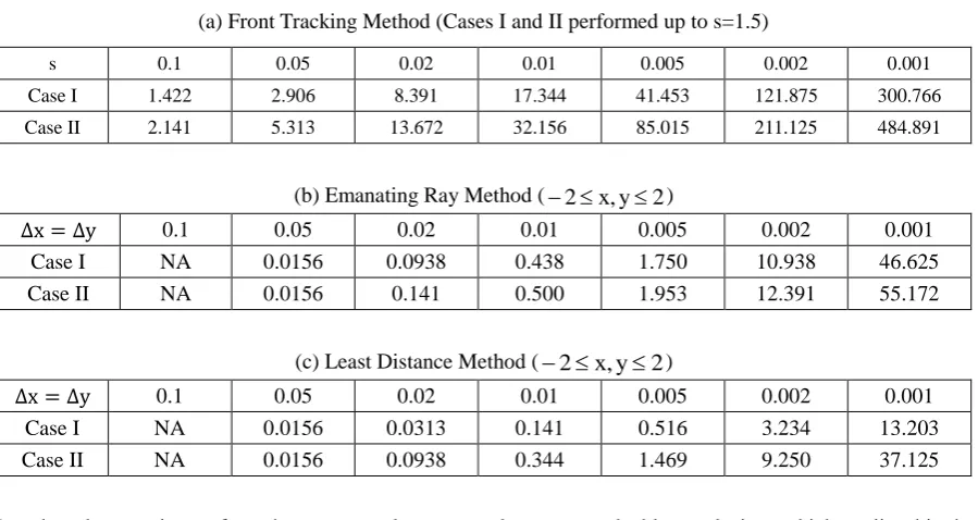
Copyright © TAETI Table 1 Comparisons of CPU times for the three proposed methods
(a) Front Tracking Method (Cases I and II performed up to s=1.5)
s 0.1 0.05 0.02 0.01 0.005 0.002 0.001
Case I 1.422 2.906 8.391 17.344 41.453 121.875 300.766
Case II 2.141 5.313 13.672 32.156 85.015 211.125 484.891
(b) Emanating Ray Method (2x,y2)
∆x = ∆y 0.1 0.05 0.02 0.01 0.005 0.002 0.001
Case I NA 0.0156 0.0938 0.438 1.750 10.938 46.625
Case II NA 0.0156 0.141 0.500 1.953 12.391 55.172
(c) Least Distance Method (
2
x
,
y
2
)∆x = ∆y 0.1 0.05 0.02 0.01 0.005 0.002 0.001
Case I NA 0.0156 0.0313 0.141 0.516 3.234 13.203
Case II NA 0.0156 0.0938 0.344 1.469 9.250 37.125
Based on the experiences from the test examples, we can draw some valuable conclusions which are listed in the Table
2. It is obviously shown that the least distance method can be chosen as a feasible method for practical grain burnback
calculation from the considerations of programming flexibility, accuracy and computational resource.
Table 2 Overall Comparisons of the advantages/disadvantages of the three proposed methods
Items Front tracking Emanating ray Least distance
Topology dependence global local no
Grid required no yes yes
Exactness straight line no nodes
Error dependence accumulated grid size grid size
Memory storage small full full
CPU time heavy mediate light
Conservation no yes yes
Extension to 3-D difficult easy straightforward
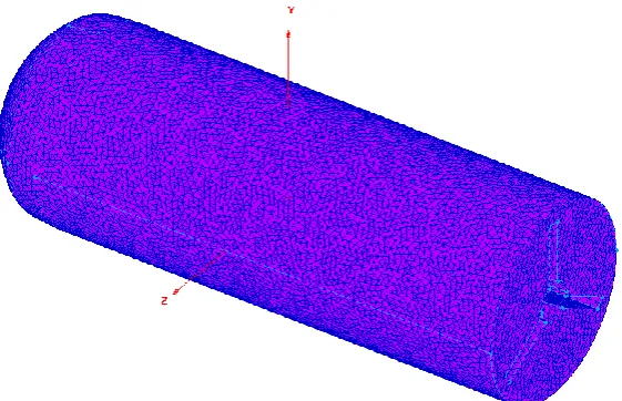
Fig. 12 Burning surfaces at different positions in Z-direction
Therefore, the least distance method is recommended to be employed to calculate the burned-volume of the
three-dimensional solid propellant at each burn distance. A simple geometry with a cubical region propagating outward is
selected as a model problem. Two different grid systems (Cartesian grids and Tetrahedron grids) have been employed. We
into N_d divisions. Therefore, N_d^3 small cubics are formed. Each small cubic can create 24 tetrahedron cells based on the
Delaunay method. The resulting burn surfaces at different positions in Z-direction by using tetrahedron cells are shown in
Figure 12. Similar contour surfaces are also observed by using Cartesian cells. It is observed the constant distance function is
symmetrically distributed with respect to the central axises. It is also shown that the sharp corners of the initial cubic region
become rounded corners as the cubic region propagates outward in all directions.
The errors in the burning volume are calculated by using the tetrahedron grids and the Cartesian grids and depicted in
the Figures 13 and 14, respectively. The errors are due to the interpolation and are relatively small. In both grid systems, our
numerical results show a promising agreement with theoretical results.
Fig. 13 Estimation of error in a three-dimensional erosive volume with respect to the burn distance by using the least distance method and tetrahedron grid system
Fig. 14 Estimation of error in a three-dimensional erosive volume with respect to the burn distance by using the least distance method and Cartesian grid system
The CPU times consumed by using the 3-D least distance method with different grid size, cell number and node
number, and with different grid systems are listed in Table 3. At each column of Table 3(a) and 3(b) the grid spacing is
comparable at the same order of magnitude for both grid systems. Apparently the calculation with the Cartesian grid is more
Copyright © TAETI Table 3 Comparison of the numerical performance for the 3-D least distance method with
the different cell and the node numbers, and different grid systems
(a) Cartesian grid (-2
x,y,z
2)Grid Size 0.1 0.05 0.02
Cells 64,000 512,000 8,000,000
Nodes 68,921 531,441 8,120,601
CPU time 1.375 10.625 162
(b) Tetrahedron grid (-2
x,y,z
2)Division (Nd) 20 40 60
Cells 192,000 1,536,000 5,184,000
Nodes 42,461 329,721 1,101,781
CPU time 0.875 6.641 21.859
Although the simulation with the Cartesian cubic cells can yield more accurate result, those with tetrahedral cells are
computationally more efficient and can still provide reasonable prediction in the test problems. Since the propellant
configuration in a practical combustor becomes complicated and difficult to simulate with a regular Cartesian grid system,
the feasibility of tetrahedral cells become quite valuable. Even with the dense grid system that has several millions of nodes,
the required CPU time is still acceptable.
4.
Conclusion Remarks and Future Work
In this paper, we present the three-dimensional numerical methods for the surface regression of the homogeneous
propellants. Three methodologies, namely the front tracking method, the emanating ray method and the least distance
method, are first proposed and verified with two two-dimensional test problems. The least distance method is found to
perform better than the other two methods in the numerical respects. A three dimensional calculation by using this method
combined with tetrahedral cells has been conducted to demonstrate its feasibility. Our preliminary result has shown a
satisfactory agreement with the theoretical data. The least distance method can be employed to a practical three-dimensional
grain design. It would require a grid generation model of the propellant topology that can completely construct the
tetrahedral cells of the grain. One of our preliminary designs looks like Figure 15. We are taking an incremental approach to
accommodate the method to the grain design. We expect our method can shorten the grain design time significantly.
References
[1] G. P. Sutton, Rocket propulsion elements: An introduction to the engineering of rockets, 6th ed. New York: John Wiley & Sons, 1992.
[2] V. Yang, T. B. Brill, W. Z. Ren, and P. Zarchan, Solid propellant chemistry, combustion, and motor interior ballistics, vol. 185. NY: American Institute of Aeronautics and Astronautics, 2000.
[3] M. J. Hyman, “Numerical Methods for Tracking Interfaces,”Journal of Computational Physics, vol. 12, no. 1-3, pp. 396-407, July 1984.
[4] S. O. Unverdi and G. Tryggvason, “A front tracking method for viscous, incompressible, multi-fluid flows,” Journal of Computational Physics, vol. 100, no. 1, pp. 25-37, May 1992.
[5] W. C. Hirt and D. B. Nichols, “Volume of fluid (VOF) method for the dynamics of free boundaries,” Journal of Computational Physics, vol. 39, no. 1, pp. 201-225, Jan. 1981.
[6] R. Scardovelli and S. Zaleski, “Direct numerical simulation of free-surface and interfacial flow,” Annual Reviews Fluid Mech, vol. 31, pp. 567-603, Jan. 1999.
[7] S. Osher, “Fronts propagating with curvature dependent speed: Algorithms based in Hamilton–Jacobi formulations,” Journal of Computational Physics, vol. 79, no. 1, pp. 12-49, Nov. 1988.
[8] O. Stanley and F. Ronald, Level set methods and dynamic implicit surfaces, applied mathematical Sciences, vol. 153. New York: Springer, 2003.
[9] N. Provatas and K. Elder, Phase-field methods in material science and engineering. Wiley, 2010.
[10] S. Chen, B. Merriman, S. Osher, and P. Smereka, “A simple level set method for solving Stefan problems,” Journal of Computational Physics, vol. 135, no. 1, pp. 8-29, July 1997.
[11] J. A. Sethian, “Curvature and the evolution of fronts,” Communications in Mathematical Physics, vol. 101, no. 4, pp. 487-499, 1985.
[12] W. J. Boettinger, J. A. Warren, C. Beckermann, and A. Karma, “Phase-field simulation of solidification,” Annual Review of Materials Research, vol. 32, pp. 163-194, Aug. 2002.
[13] R. Kobayashi, “Modeling and numerical simulation of dendritic crystal growth,” Physica D: Nonlinear Phenomena, vol. 63, no. 3-4, pp. 410-423, Mar. 1993.
[14] V. R. Voller and C. Prakash, “A fixed grid numerical modeling methodology for convection-diffusion mushy region phase-change problems,” International Journal of Heat and Mass Transfer, vol. 30, no. 8, p. 1709-1719, Aug. 1987. [15] L. W. Hunter and J. R. Kuttler, “Enthalpy method for ablation-type moving boundary problems,” Journal of
Thermophysics and Heat Transfer, vol. 5, no. 2, pp. 240-242, 1991.
[16] G. Püskülcü and A. Ulas, “3-D grain burnback analysis of solid propellant rocket motors: Part 2 – modeling and simulations,” Aerospace Science and Technology, vol. 12, no. 8, p. 585-591, Dec. 2008.
[17] X. Wang, T. L. Jackson, and L. Massa, “Numerical simulation of heterogeneous propellant combustion by a level set method,” Combustion Theory and Modelling, vol. 8, no. 2, pp. 227-254, 2004.
[18] M. A. Wilcox, M. Q. Brewster, K. C. Tang, D. C. Stewart, and I. Kuznetsov, “Solid rocket motor internal ballistics simulation using three-dimensional grain Burnback,” Journal of Propulsion and Power, vol. 23, no. 3, pp. 575-584, 2007.
[19] C. Yildirim and M. H. Aksel, Numerical simulation of the grain. Burnback in solid propellant rocket motor. American Institute of Aeronautics and Astronautics, July 2005.