Nonlinear controller tuning based on a sequence of identifications of linearized time-varying models

Nonlinear controller tuning based on a sequence of identifications

of linearized time-varying models

Jonas Sjo¨berg

a

, Per-Olof Gutman

b,

, Mukul Agarwal

c

, Mike Bax

d

a

Department of Signals and Systems, Chalmers University of Technology, 412 96 Gothenburg, Sweden b_{Faculty of Civil and Environmental Engineering, Technion—Israel Institute of Technology, Haifa 32000, Israel} c

Bu¨hler AG, CH-9240 Uzwil, Switzerland d

Department of Mechatronics, Philips Applied Technologies, 5656 AE Eindhoven, The Netherlands

a r t i c l e

i n f o

Article history:

Received 5 October 2007 Accepted 5 August 2008 Available online 11 October 2008

Keywords: Nonlinear control Controller tuning Optimization

Control-oriented identification

a b s t r a c t

A novel algorithm for tuning controllers for nonlinear plants is presented. The algorithm iteratively minimizes a criterion of the control performance. In each iteration one experiment is performed with a reference signal slightly different from the previous reference signal. The input–output signals of the plant are used to identify a linear time-varying model of the plant which is then used to calculate an update of the controller parameters. The algorithm requires an initial feedback controller that stabilizes the closed loop for the desired reference signal and in its vicinity, and that the closed-loop outputs are similar for the previous and current reference signals. The tuning algorithm is successfully tested on a laboratory set-up of the Furuta pendulum.

&2008 Published by Elsevier Ltd.

1. Introduction

Most methods for controller tuning rely on a mathematical model of the plant. The model is necessary to calculate the derivative of the output signal with respect to the controller parameters. See, e.g.,Trulsson and Ljung (1985)on linear systems and, e.g.,Harris (1994)on nonlinear systems. In this contribution a novel approach is presented: instead of identifying a, more or less, global nonlinear model of the plant, a linear time-varying model is identified along a trajectory of the plant. The time-varying model is then used to compute the derivative of the plant output with respect to the controller parameters. Since the model is valid only for a particular trajectory, the identification step has to be repeated in each iteration, i.e., after each change of the controller parameters.

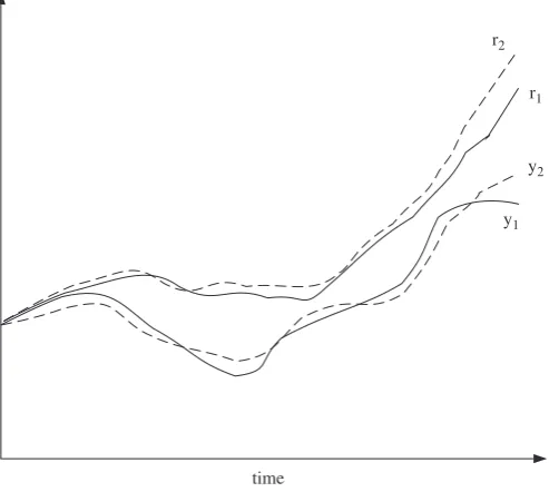
The algorithm requires an initial, parameterized, feedback controller that stabilizes the closed loop for the desired reference signal and in its vicinity. This is illustrated inFig. 1. It is also assumed that the plant can be described locally by a linear model which may be slowly time-varying along the considered neigh-boring trajectories. The proposed algorithm is then used to tune the controller parameters so that a control goal is optimized.

The algorithm is described by the following steps.

Algorithm 1.1. Basic steps for tuning the controller.

1. Perform one experiment on the plant with a desired reference signal.

2. Identify a linear time-varying plant model describing the input–output data.

3. Use the model to compute the derivative (with respect to the controller parameters) of the criterion of the control objective along the trajectory.

4. Update the controller parameters.

5. Repeat from step1if the control objective is not satisfied.

The user has to choose a linear model structure for the plant and an identification method with which to identify its time-varying parameters. It is then assumed that the reference signal and the sequence of updated feedback controllers are such that the plant input signal becomes persistently exciting in order to ensure identifiability of the plant model parameters.

The linearization of the plant must change slowly during an experiment, otherwise it is not possible to obtain a good linear time-varying model. This can be assured if the reference signal is changing slowly between different operating regimes, i.e., if it is dominated by low frequencies. However, there must be some high frequency contents of low amplitude, otherwise the dynamics cannot be identified.

It should be noted that the identification of the linear time-varying model is done off-line. This implies that, in contrast to normal recursive identification, not only preceding but also Contents lists available atScienceDirect

journal homepage:www.elsevier.com/locate/conengprac

Control Engineering Practice

0967-0661/$ - see front matter&2008 Published by Elsevier Ltd. doi:10.1016/j.conengprac.2008.08.001

Corresponding author. Tel.: +972 4 8292811.

E-mail addresses:[email protected] (J. Sjo¨berg),

[email protected] (P.-O. Gutman),

successive data are used to obtain a model at timet. Hence, the model quality and the tuning is improved.

The optimization is done with respect to a desired reference signal and the obtained controller is then optimal only for this specific reference signal. Above it was assumed that the initial stabilizing controller caused the closed-loop outputs to be similar for reference signals in the neighborhood of the desired reference signal. If this property is retained for the optimized controller then this controller will be nearly optimal also for reference signals in the mentioned neighborhood.

The problems for which the results of this paper may be useful include the following:

In batch processes, e.g., in the chemical industry, it is common that a controlled variable, e.g., temperature, has to track a given reference trajectory. When a model of the process is unavailable or only known with large uncertainty, but the process is equipped with a functioning feedback controller, the proposed procedure may be used to optimize the controller. In Sjo¨berg and Agarwal (1998)an example of this is given.

A common form of adaptive control is the so-called gain

scheduling (Astro¨m & Wittenmark, 1995) whereby different controllers have been designed for a number of operating points. When the actual operating point is at or near a design operating point the corresponding controller output is input to the plant. The present procedure may be used to tune controllers optimized for a number of reference trajectories, thus constructing a trajectory-dependent gain scheduling. An example of gain-scheduling controller tuning is given in Section 7. It should, however, be pointed out that gain scheduling may be non-trivial for, e.g., multiple model

systems or linear time-varying systems, see, e.g.,

Murray-Smith and Johansen (1997)andJohansen and Foss (1999)and

other articles in that special issue, and Leith and Leithead

(2000).

The proposed method can also be used to tune linear

controllers in connection with nonlinear plants. For example, the commonly used PI- and PID can be tuned in this way. The second example in Section 7 demonstrates PID-tuning for the

Furuta pendulum (Astro¨m & Furuta, 2000; Furuta, 2003; Furuta, Yamakita, & Kobayashi, 1991; Furuta, Yamakita, Kobayashi, & Nishimura, 1991).

Under the assumption that a controller is known to globally

stabilize the plant when the controller parameters belong to a set, one could use the procedure in this paper to tune the parameter values with respect to a number of reference trajectories that are weighted into one criterion. One optimized global controller is then obtained.

The current method, a preliminary version of which was

presented asSjo¨berg and Agarwal (1997), can be compared with

many contributions in the control literature. Since the model is valid only locally around a trajectory, the new algorithm can be seen as a special case ofmodeling for control. However, most other works on modeling for control address the frequency contents of

the input signal for linear systems, see, e.g., Gunnarsson and

Hjalmarsson (1994), Astro¨m and Nilsson (1994) and Gevers (1993). The algorithm presented in this paper can be seen as a novel type of identification for control where the time-varying identification is a way to take nonlinearities of the plant into account.

Iterative feedback tuning is suggested for linear systems in Hjalmarsson, Gevers, Gunnarsson, and Lequin (1998) and Hjalmarsson, Gunnarsson, and Gevers (1995), where instead of using a model, three experiments are performed in each iteration. For nonlinear plants that method requires in each iteration a

number of experiments equal nþ1 or nþ2, where n is the

number of controller parameters, seeSjo¨berg and Agarwal (1996), De Bruyne, Anderson, Gevers, and Linard (1997)orSjo¨berg et al. (2003). If the controller contains many parameters this may be too many experiments to be applicable. The model-based tuning algorithm presented here is a way to reduce the number of experiments in each iteration to one. The proposed method has several user aspects in common with iterative feedback tuning. For example, none of the methods give any guarantees for closed-loop stability. Instead, if stability is a problem, then this has to be

assured using some additional method. SeeHjalmarsson et al.

(1998)for a discussion on such issues.

The present contribution can be seen as an extension of Sjo¨berg et al. (2003). The difference is that here one experiment per controller update iteration is needed to identify a time-varying linear plant model in order to compute the derivatives of the output with respect to the controller parameters, while the method inSjo¨berg et al. (2003)is model free, but, as mentioned

above, requires nþ1 or nþ2 experiments per iteration to

compute the derivatives. Otherwise the two methods are identical. Common issues and assumptions associated with the iterative combination of identification, derivative estimation, and control design within a noisy and nonlinear dynamic context are mostly treated inSjo¨berg et al. (2003).

There is also a close connection toextremum control(Astro¨m & Wittenmark, 1995; Sternby, 1980; Wittenmark & Urquhart, 1995) which is a type of adaptive control where an on-line search in the controller parameter space is conducted in order to minimize a criterion. If the method is applied to tune the controller parameters on-line it becomes an extremum controller. The advantage of the new algorithm is that it does not require the controller parameters to be moved away from the optimum in order to compute the derivative of the criterion with respect to the controller parameters which is the case with conventional extremum control.

Finally, there is a connection toquantitative feedback theoryfor

smooth nonlinear systems, seeHorowitz (1982, 1992), in which

linear input–output transfer function models are identified for r1

r2

y1

y2

[image:2.595.36.283.74.295.2]

time

different desired outputs of the uncertain nonlinear plant. Based on these models, one linear controller is designed which is robust both with respect to performance and stability, using a proof based on Schauder’s fixed point theorem. As suggested in point three above, the method could be used to design and optimize a robust controller.

The novel idea in this paper is hence to use a linear time-varying description instead of a global nonlinear model, or no model at all, to compute the derivatives of the output with respect to the controller parameters. The great advantage lies in the fact that linear models are easier to specify whereas global nonlinear descriptions require considerable insight into the plant behavior, and numerous experiments. However, if a good global nonlinear model can be obtained it is probably better to use parametric

optimization methods as described in, e.g., Harris (1994) and

Monje, Vinagre, Feliu, and Chen (2008). Such a model can, of course, also be expanded as a linear time-varying model along a trajectory, see, e.g.,Hu, Kumamaru, and Inoue (1996).

The paper is organized in the following way. In Section 2 the problem formulation and the control objective are stated. In Section 3 a time-varying description of a nonlinear plant is given. How to obtain the derivative of the output with respect to the control parameters is described in Section 4, and different possibilities for parameterizing the linear time-varying model are presented in Section 5. Advantages and limitations of the proposed scheme are discussed in Section 6. Two application examples are given in Section 7, including laboratory experiments with the Furuta pendulum. The paper is concluded in Section 8.

2. Control objective and problem formulation

Given a nonlinear plant, assume there exists a controller of the following form:

uðtÞ ¼gð

r;

yðtÞ;yðt1Þ;. . .;yðtnyÞ;uðt1Þ;. . .;uðtnu1Þ,

rðtÞ;. . .;rðtnrÞÞ, (1)

which stabilizes the plant for some initial controller parameter vector value

r

¼

r

0. The control signal uðtÞdepends on present

and past plant outputs y and reference signals r. The initial

controller with

r

¼

r

0 as well as the updated vectors

r

i, i¼

1;2;. . .are assumed to stabilize the system along the trajectory of an experiment. The goal is then to tune

r

so that the performance of the controller is optimized with respect to some criterion.

By the Internal Model Principle, as expressed, e.g., inMorari and Zafiriou (1989), it follows from the assumption that the closed-loop system is stabilized by the initial controller, that the plant can be described by

zðtÞ ¼fðzðt1Þ;. . .;zðtnzÞ;uðt1Þ;. . .;uðtnu2ÞÞ,

yðtÞ ¼zðtÞ þ

n

ðtÞ, (2) wherefðÞis an unknown nonlinear function and

n

ðtÞ is a zero-mean, not necessarily white, noise signal. This description also follows from an extension of the Takens embedding theorems (Stark, 1999; Stark, Broomhead, Davies, & Huke, 1997). Compare also withHorowitz (1992, 309pp). It will also be assumed thatfðÞ is a smooth function. The integersnzand nu2 are unknown, but they are related to the number of known shifts in the stabilizing controller,nrandny. By the Internal Model Principle, one may, e.g.,

letnz¼nyandnu2¼nr.

2.1. The control criterion and its minimization

Let the desired plant output be described as a filtered version of the reference signal

ydðtÞ ¼TdrðtÞ.

The filterTdis typically linear time-invariant, but it could also be

nonlinear or time-varying.

A natural design objective is to minimize some norm of the deviation of the plant output yðtÞ from the desired output ydðtÞ.

Indicating this norm by Jð

r

Þ the desired value of the controller parameters becomes

r

_¼argmin

r Jð

r

Þ. (3)

The criterionJcould be any measure of the fit. In this contribution, however, the attention is restricted to quadratic measures of the form

Jð

r

Þ ¼X

t

1

2E½ðLyðyð

r

Þ ydÞÞ

2

þ

g

2E½ðLuuð

r

ÞÞ

2

, (4)

where the expectations are with respect to the noise

n

ðtÞin (2). The

design parameter

g

is used to monitor the trade-off between

performance and control effort. The filtersLyandLucan be used to

emphasize certain frequencies. They will be set to unity in the sequel since they do not change the general derivation of the algorithm.

To minimize (4), the following equation must be solved with respect to

r:

0¼J0

ð

r

Þ ¼E½ðyð

r

Þ ydÞy0ð

r

Þ þ

g

E½uð

r

Þu0ð

r

Þ (5)

which is done by a numerical search

r

iþ1¼

r

i

m

iR 1

i J 0

ð

r

iÞ. (6)

In each iteration i the parameters are changed in a descent

direction. The matrix Ri is typically an approximation of the

Hessian matrix which changes the search from the steepest-descent to a more favorable direction (Dennis & Schnabel, 1983). The step length

m

i should be chosen so that a down-hill step is

obtained. Conditions for convergence to a local minimum are briefly discussed inSjo¨berg et al. (2003). A discussion about the rate of convergence is outside the scope of this paper, instead see, e.g.,Dennis and Schnabel (1983).

The tricky part in (5) and (6) is the computation of the derivatives y0_ð

_r

_{Þ of the output and u}0_ð

_r

_{Þ of the control signal.}

The contribution of this paper is to obtain an estimate of the derivatives by linearized time-varying modeling of the plant. Notice that since the model is valid only along a particular

trajectory, which in turn depends on

r, the modeling has to be

repeated in each iteration of (6).

3. Linearized time-varying description of the plant

In this section the linearized time-varying description of the plant is given. This description is then used in the following section to obtain an expression for the derivative of the plant output and the control action with respect to the controller parameters.

The changes of the trajectories of an experiment due to a small perturbation of the controller parameters are described with Taylor expansions. The expressions for the derivatives are then obtained by letting the parameter perturbation go to zero. It will be shown that when the algorithm is used, no experimental change of the parameter vector is necessary in order to obtain the derivatives.

Given a reference signalfriðtÞgNt¼1consisting ofNtime samples, an

experiment labeledican be performed on the plant with the current controller parameters

r

i. This gives trajectories of the plant output

fyiðtÞgNt¼1 and of the control signal fuiðtÞgNt¼1. Introducing the

following variables as differences fromfyiðtÞ;uiðtÞ;riðtÞg:

D

yðtÞ ¼yðtÞ yiðtÞ,

D

uðtÞ ¼uðtÞ uiðtÞ,

D

zðtÞ ¼zðtÞ ziðtÞ,

D

r

ðtÞ ¼

r

ðtÞ

r

iðtÞ. (7)

The output (2) can be described as

yðtÞ ¼ziðtÞ þ

D

zðtÞ þ

n

ðtÞ. (8)

The plant (2) is assumed to be smooth. Hence, iff

D

zðtnÞgnz

n¼1and

f

D

uðtnÞgnu2

n¼1 are small then (2) can be expressed by a Taylor

expansion aroundziðtÞanduiðtÞ

zðtÞ ¼ziðtÞ þ

Xnz

n¼1

q

fðÞ

q

zðtnÞ

D

zðtnÞ

þX

nu₂

n¼1

q

fðÞ

q

uðtnÞ

D

uðtnÞ þOð

D

2

maxÞ, (9)

where the partial derivatives are evaluated at fziðtnÞgnn¼z1 and

fuiðtnÞg nu₂

n¼1. The higher order terms are described by Oð

D

2 maxÞ,

where

D

max indicates the largest

D

in the equation, andOðxÞ !0

when x!0. This expression can be found for each t of the

experiment, and an expansion of the function fðÞ along the

trajectory fziðtÞ;uiðtÞgNt¼1 is obtained. Of course, since fziðtÞgNt¼1 is

not available, and the systemfðÞis unknown, the expansion is only a formal description. Instead, the idea is to identify the partial derivatives in (9) by using experimental data. This is discussed in the next section.

In the same way as the plant was linearized, the controlleruðtÞ in (1) can also be expressed by a Taylor series around fyiðtÞ;uiðtÞ;riðtÞgNt¼1and

r

i

uðtÞ ¼uiðtÞ þ

Xny

n¼0

q

gðÞ

q

yðtnÞ

D

yðtnÞ þ

Xnu₁

n¼1

q

gðÞ

q

uðtnÞ

D

uðtnÞ

þX

nr

n¼0

q

gðÞ

q

rðtnÞ

D

rðtnÞ þgðfyi;ui;rigÞ

0

D

r

þOð

D

2maxÞ, (10)

wheregðfyi;ui;rigÞ0 is the partial derivative of the control signal

with respect to the parameters

r

evaluated along the trajectory

fyiðtÞ;uiðtÞ;riðtÞgNt¼1.

The relation between

D

rðtÞ,

D

uðtÞ, and

D

yðtÞ can now be described as a time-varying system. To see this the following notation is introduced:

F¼Fðt;q1_Þ¼: 1

AB,

A¼:1fz1ðtÞq1 fz nzðtÞq

nz_,

B¼:fu1ðtÞq1þ þfu nu2ðtÞq

nu2,

R¼:1gu1ðtÞq1 gu nu₁ðtÞq

nu_1,

S¼: gy0ðtÞ gy1ðtÞq1 gy nyðtÞq

ny_,

T¼:gr0ðtÞ þgr1ðtÞq1þ þgr nrðtÞq

nr_{, (11)}

where q is the shift operator, i.e., q1_{uðtÞ ¼uðt1Þ, and the}

partial derivatives, evaluated along the trajectoriesfziðtÞ;uiðtÞgNt¼1

and fyiðtÞ;uiðtÞ;riðtÞgNt¼1, have been abbreviated in the following

way:

fz nðtÞ¼:

q

fðÞ

q

zðtnÞ

_fz

iðtnÞnzn¼1;uiðtnÞ nu2

n¼1g ,

fu nðtÞ¼

:

q

fðÞ

q

uðtnÞ

fziðtnÞnzn¼1;uiðtnÞ nu₂ n¼1g

,

gy nðtÞ¼:

q

gðÞ

q

yðtnÞ

fyiðtnÞ ny n¼0;uiðtnÞ

nu₁

n¼1;riðtnÞnrn¼0;r¼rig ,

gu nðtÞ¼:

q

gðÞ

q

uðtnÞ

_fy

iðtnÞnyn¼0;uiðtnÞ nu1

n¼1;riðtnÞnrn¼0;r¼rig ,

gr nðtÞ¼

:

q

gðÞ

q

rðtnÞ

fyiðtnÞ ny n¼0;uiðtnÞ

nu₁

n¼1;riðtnÞnrn¼0;r¼rig

. (12)

Note thatF,A, andBare unknown sincefis unknown, whileR,S,

andTmay be computed from the knowng. The new notation and

the Taylor expansions (9) and (10) give the linearized time-varying system

D

zðtÞ ¼F

D

uðtÞ þOð

D

2

maxÞ,

D

yðtÞ ¼

D

zðtÞ þ

n

ðtÞ þOð

D

2maxÞ (13)

and the linearized time-varying controller

D

uðtÞ ¼1

Rðgðfyi;ui;rigÞ0

D

r

S

D

yðtÞ þT

D

rðtÞÞ þOð

D

2maxÞ. (14)

Plugging in the control signal (14) in the plant equation (13) gives us the linearized closed-loop system

D

yðtÞ ¼F1

Rðgðfyi;ui;rigÞ0

D

r

S

D

yðtÞ þT

D

rðtÞÞ þ

n

ðtÞ þOð

D

2maxÞ.

(15)

This relation will be used to obtain expressions for the derivatives of the output and the control signal.

4. The output and input derivatives

In this section it is demonstrated how the output and input derivatives with respect to the controller parameters can be obtained using the linearized system description from the previous section.

Once the trajectoriesfyiðtÞ;uiðtÞ;riðtÞgNt¼1andfziðtÞ;uiðtÞgNt¼1have

been obtained in an experiment, they are used merely as a series of points around which the Taylor expansions (9) and (10) are computed. This means thatyiðtÞin (7) does not depend on

r

and,

hence, the derivative of the linearized plant becomes identical with the derivative of the original plant (2), i.e.,

y0_ðtÞ dy

dr¼

d

D

y

d

D

r

D

y

0_ðtÞ.

Using this relation the derivative with respect to controller parameters can be obtained using the linear time-varying plant. Taking the derivative of (15) with respect to

D

r

gives

D

y0_{ðtÞ ¼F}1

Rðgðfyi;ui;rigÞ

0

S

D

y0_{ðtÞÞ þOð}

_D

maxÞ. (16)

This gives us the following expression for the derivative:

y0

ðtÞ ¼ 1 1þF1

RS

F1

Rgðfyi;ui;rigÞ

0

þOð

D

maxÞ. (17)

If the control-signal penalty

g

is non-zero in the control

criterion (4), then the derivative of the control signal is also needed and it can be obtained from (14)

u0_{ðtÞ ¼}

_D

_u0_{ðtÞ ¼}1

Rgðfyi;ui;rigÞ

0

1

RSy

0

ðtÞ þOð

D

maxÞ. (18)

This expression also follows directly from the original expression of the controller (1).

Since

D

max may be chosen arbitrary small, the error terms in

(17) and (18) can be made arbitrary small. Hence, the exact expressions of the derivatives of the output and the control signal with respect to the controller parameters are obtained from (17) and (18) by setting the error terms to zero.

The only practical problem which prevents us from using (17) and (18) directly is that using the time-varying plant description,

F, is not known. In the following section possibilities for

5. The linear time-varying model

After having derived expressions (17) and (18) for the output and control derivatives it remains to specify how the linear time-varying filterð1=ð1þFð1=RÞSÞÞFð1=RÞ should be obtained in each iteration of the tuning algorithm. This is a design step and there are many different approaches. The best choice depends on the problem at hand, and a rather general discussion about the different possibilities will be given. One possible design approach will then be discussed in more detail.

A general requirement for the tuning method to be applicable is that it is possible to obtain a good time-varying model. This is possible if the the time-varying description of the plant (13) changes slowly with time, i.e., if there is a small change of the linear description between consecutive time samples. This can be described by considering the frequency contents of the reference signal.

Assume that the reference signal is dominated by low

frequencies superimposed with a high frequency part of smaller amplitude. Then the linearization of the system depends on the low frequency component which describes a changing operating point of the system. The high frequency part of the reference signal describes deviations around the low frequency part, and if the amplitudes of these deviations are small, then the they will only influence the linearization marginally.

Using this frequency description of the reference signal, it follows that the high frequency component is necessary to obtain

excitation of the dynamic of the system. Refer toLjung (1999)

for a discussion on the necessity and choice of ‘‘persistently exciting’’ excitation signals.

Consider now the time-varying description (17). In principle,

only the unknownFin (17) needs to be estimated, sinceRandS

can be computed by definition (12). However, it is also possible to estimate the closed-loop systemð1=ð1þFð1=RÞSÞÞFð1=RÞdirectly, as shown in the simulation example in Section 7. These two possibilities merely represent different ways of closed-loop identification; general aspects on closed-loop identification are

discussed in, e.g., den Hof and Schrama (1995) and Fogel and

Huang (1982).

The expression for the time-varying system (13) can be re-written as

yðtÞ ¼yiðtÞ þ

D

yðtÞ ¼yiðtÞ þFð

D

uðtÞ þuiðtÞ uiðtÞÞ þ

n

ðtÞ þOð

D

2maxÞ

¼yiðtÞ þFuðtÞ FuiðtÞ þ

n

ðtÞ þOð

D

2maxÞ

¼FuðtÞ þ

n

ðtÞ þb0ðtÞ þOð

D

2maxÞ, (19)

whereb0ðtÞ ¼yiðtÞ FuiðtÞis a time-varying parameter describing

the DC-level of the output signal, i.e., it describes the influence of the low frequency part of the reference signal. The derivations above leading to (19) can easily be extended to include the case of filtered noise rather than the assumed output noise. Therefore relationship (19) can be modeled by a general linear time-varying model given by

yðtÞ ¼Gðt;q1

ÞuðtÞ þHðt;q1

ÞeðtÞ þb0ðtÞ, (20)

whereGðt;q1_{Þ is the plant dynamics and Hðt;q}1_{Þ is the noise}

dynamics at timet. The DC-level parameterb0ðtÞcorresponds to

the operating point around which the linearization is done at time

t. Hence,b0ðtÞis a special type of parameter and in some situations

it should be handled differently from the other parameters. It is, for example, possible that b0ðtÞ changes fast at certain time

instances as the response to fast changes in the reference signal. Then a possible solution is to perform two experiments with

similar reference signals and to form

d

r¼r1ðtÞ r2ðtÞ,

d

y¼y1ðtÞ

y2ðtÞ etc., and to use the

d

data sequences in the identification.

Then the parameter b0ðtÞ does not have to be included in the

model, since its contribution is canceled in the subtraction of the signals from the two experiments, i.e., (20) can be replaced by

d

yðtÞ ¼Gðt;q1_Þ

_d

_{uðtÞ þHðt;q}1_{ÞeðtÞ. (21)}

In some situations there might be prior knowledge available to guide the choice of Gðt;q1_{Þ and Hðt;q}1_{Þ. Otherwise one can}

choose a black-box model structure such as ARX, OE, ARMAX, or BJ. See, e.g.,Ljung (1999).

Here the general discussion is concentrated on the time-varying ARX model

yðtÞ ¼1

ABuðtÞ þ

1

AeðtÞ þb0ðtÞ (22)

with

A¼1þa1ðtÞq1þ þanaðtÞq

na_,

B¼bnkðtÞq

nk_{þ þb}

nkþnb1qnknbþ1,

where na,nb, and nk specify the model orders and time delay,

respectively. This can also be described as a time-varying linear regression

yðtÞ ¼

y

TðtÞ

j

ðtÞ (23) with

y

ðtÞ ¼ ½a1ðtÞ;. . .;anaðtÞ; bnkðtÞ;. . .;bnkþnb1ðtÞ; b0ðtÞ

T

and

j

ðtÞ ¼ ½yðt1Þ;. . .;yðtnaÞ; uðtnkÞ;. . .;uðtnknbþ1Þ; 1T.

Note the 1 in the last position of the regressor. It has been included so thatb0ðtÞ can be estimated together with the other

parameters.

The typical way to estimate time-varying models with noisy measurements is to use a recursive estimation algorithm like the Kalman filter or recursive least squares with a forgetting factor.

See, e.g.,Ljung and Soderstrom (1983)andAnderson and Moore

(1979). Issues related to the validity of the model, influence of measurement noise and choice of excitation signal are also addressed in, e.g., Ljung (1999) and Sjo¨berg et al. (2003). Here there is an off-line situation. All data are available for identifica-tion, not only those for time samples up tot. Hence, there is no need to use a recursive algorithm just because the system description (20) is time-varying. Instead the parameters in (23) can be described as basis function expansions. For example, the parametera1ðtÞcan be expanded as

a1ðtÞ ¼

Xn

k¼1

a1khkðtÞ, (24)

wherefhkðtÞgnk¼1are the basis functions andfa1kgnk¼1are the new,

time-invariant parameters. This is actually a re-parameterization of the model where the time-dependence is separated from the parameters. The basis expansion should be chosen so that the time dependent variation is largest where the changes in the plant dynamics are largest. For example, if it is known that the reference signal jumps from one level to another at some time instantt0and

that the reference signal is relatively constant before and after this jump, then this motivates the following two basis functions:

h1ðtÞ ¼

1; tot0;

0; tXt₀; (

h2ðtÞ ¼

0; tot0;

1; tXt₀: (

Another approach, suggested in the example in Section 7, is to use a weighted criterion (Ljung, 1999), such that the observations around timetare more important than other observations for the estimation of the parameter values att. The parameters attare then obtained by minimizing the criterion

Vðt;

y

Þ ¼ 1 2N

Xt

i¼1

l

ti_t ½yðiÞ

y

TðiÞ

j

ðiÞ2þ 1 2N

XN

i¼tþ1

l

it_t ½yðiÞ

y

TðiÞ

j

ðiÞ2.

(25)

Note that the first term of the right-hand side corresponds to the recursive least squares with forgetting factor (Ljung, 1999). The forgetting factor

l

tp1 can be different for differentt. This gives us

the possibility to have more local models where the dynamics change fast and vice versa. It is also possible to choose shapes for the time-window other than the exponential one, e.g., a rectangular window could be possible.

The choice of

l

tin (25) gives a bias–variance trade-off for the

time-varying model. With

l

t¼1 the model becomes

time-invariant and the parameters are supported equally by all data. For

l

to1 the data close totgives a larger contribution to the fit

than those far away. A lower

l

t-value gives less bias and higher

variance in the parameter estimate.

The choice of

l

t is also guided by the controller structure (1).

The bias–variance trade-off in the modeling is just an inter-mediate step of the tuning of the controller parameters and it is the variance and bias of the controller parameters which are of primary interest. Hence, a small value of

l

t, giving a noisy model

estimate, can be accepted if the time-varying model is used to estimate a controller with a low number of parameters.

Notice that this claim only holds if all the control parameters influence the controller for all, or at least many, of the time samples in the trajectory. For example, an adaptive pole place-ment controller, see, e.g.,Astro¨m and Wittenmark (1995)does not have this feature, the controller at a giventdepends only on the

current model at t. Hence, for an adaptive pole placement

controller the error in the parameters at timetcarry over directly to the control parameters.

On the other hand, if the controller is, in some sense, globally

parameterized so that the controller parameters at a given t

depend on the model at many different t values, then the

influence of the model-parameter variance will decrease. The reason for this is that the controller parameters are a function of, loosely speaking, the mean value of several models at differentt

values. So for globally parameterized controllers one can use a lower value of

l

tsince the variance contribution is averaged out.

This gives a possibility to reduce the bias without increasing the variance in globally parameterized controllers.

6. Discussion

The traditional alternative to the proposed algorithm is to identify a global nonlinear model which can be used for the tuning. What are the advantages and disadvantages of the two methods? If a good global model is available, then it is probably a good idea to use it; if not, the proposed algorithm might be a useful alternative.

The main advantage with the proposed method is probably that the plant behavior is modeled only around the trajectory where it is needed. There are no parameters or data wasted on estimating the plant away from the trajectory. Choosing a nonlinear model structure is in many cases a very delicate matter. In some applications there is enough prior knowledge to construct a physical model that is parsimonious in the number of unknown parameters. However, in many applications one has to play around with nonlinear black-box models. Since there are many

more possible choices for nonlinear black-box models than for linear ones it can be a time consuming and tedious task to find an appropriate structure—if at all possible. See, e.g., Sjo¨berg et al. (1995)andCao, Rees, and Feng (1997a, 1997b)for aspects on this. Hence, the proposed method can be seen as a way to avoid the nonlinear identification problem. Instead of choosing an appro-priate nonlinear model structure one has to choose among the family of linear time-invariant model structures (20). This is generally a much easier task. If criterion (25) is used, then in addition to the model structure, the forgetting factor

l

thas to be

decided upon. However, as described in the previous section, if the controller is globally parameterized, the controller is expected to be robust with respect to the exact choice of

l

t.

A mixture of the two methods would be to update a global model in each iteration of (6). This corresponds to iterative identification for control in the linear case, described in, e.g., Gunnarsson and Hjalmarsson (1994).

It is, of course, possible to generalize the proposed algorithm and to include the results from several experiments in each iteration of the controller parameter update. Depending on the nature of the different trajectories this can give a more ‘‘global’’ controller spanning all the used trajectories. Such an approach would give a series of trajectories frkðtÞg along which the

derivative J0

ð

r

Þ of the control criterion is computed. The total criterion is then a weighted sum of the performances along the different trajectories. Note that if the unperturbed reference trajectory is chosen to be constant, rkðtÞ ¼rk, then a

time-invariant linear model will be obtained.

7. Two examples

In Sjo¨berg and Agarwal (1998), a simulation example can be found where the algorithm is used to tune the controller of a chemical batch reactor. Here, another two examples are given. The first example illustrates, by simulation, the possible use of the algorithm to tune a gain-scheduling controller for a small nonlinear plant; the second example shows the tuning of a PID controller for a laboratory set-up of the Furuta pendulum.

7.1. Gain scheduling for a nonlinear plant

The plant is described by the following equation:

yðtÞ ¼ ð1

s

ðtÞÞð1:5yðt1Þ 0:56yðt2ÞÞ

þ

s

ðtÞð3yðt1Þ 2:26yðt2ÞÞ þuðt1Þ þ

n

ðtÞ, (26) where

n

ðtÞis Gaussian white noise with standard deviation 0.05, and

s

ðtÞ ¼ 1

1þexpð2pffiffiffiffiffiffiffiffiffiffiffiffiffiffiffiffiffiffiffiffiffiffiffiffiffiffiffiffiffiffiffiffiffiffiffiffiffiffiffiffiffiffiffiy2_{ðt1Þ þy}2_ðt2Þþ8Þ.

Note that the noise in (26) enters as process noise in violation with the measurement noise assumption in (2). This makes the illustration slightly more realistic, although the noise level is low. The desired closed-loop system is specified as

ydðtÞ ¼

0:3

10:9q1_þ0:2q2rðt1Þ (27)

which is a low pass filtering ofrðtÞwith poles at 0.4 and 0.5. For small values of yðtÞ one has

s

ðtÞ 0 and the plant is approximately linear,

yðtÞ 1:5yðt1Þ 0:56yðt2Þ þuðt1Þ þ

n

ðtÞ.

For large values of yðtÞ it holds that

s

ðtÞ 1 and the linear difference equation

These linear approximations motivate control laws that place the dominant closed-loop poles at f0:4;0:5g according to (27). One gets

u1ðtÞ ¼ 0:6yðtÞ þ0:36yðt1Þ þ0:3rðtÞ (28)

for small values ofyðtÞ, and

u2ðtÞ ¼ 2:1yðtÞ þ2:06yðt1Þ þ0:3rðtÞ (29)

for large values ofyðtÞ.

A gain-scheduling controller (Astro¨m & Wittenmark, 1995),

ugðtÞis then designed by combining the linear control lawsu1ðtÞ

andu2ðtÞas

ugðtÞ ¼ ð1kÞu1ðtÞ þku2ðtÞ, (30)

where

k¼

0 ifyðtÞp1;

ðyðtÞ 1Þ=3 if 1oyðtÞo4;

1 ifyðtÞX4:

8 > < > :

The desired outputydðtÞis obtained according to (27) whererðtÞis

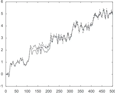
a sum of a low- and a high-frequency signal. The low frequency part ofrðtÞconsists of a sum of five unit steps, att¼10, 110, 210, 310, and 410, and the high frequency part is white Gaussian noise with standard deviation 0.5. In Fig. 2ydðtÞis depicted together

with the closed-loop output usingugðtÞ (30) to control system

(26). It is clear that the performance is better at high and low amplitudes where the linear approximations hold.

The goal is now to find better parameter values for the gain scheduling controller. The linear controllers (28) and (29) give rise to the initial parameter value vector

r

0¼ ½0:6 0:36 0:3 2:1 2:06 0:3.

The control performance criterion is chosen

Jð

r

Þ ¼X

t

ðydðtÞ yðtÞÞ

2

.

To compute the derivative of the plant output with respect to the controller parameters using expression (17), the controller derivative along the trajectory and the time-varying filterð1=ð1þ

Fð1=RÞSÞÞFð1=RÞare needed. Using (30), (28), and (29) one obtains

gðfyi;ui;rigÞ0¼ ½ð1kÞ½yðtÞ yðt1Þ rðtÞ k½yðtÞ yðt1Þ rðtÞ.

Instead of estimating a time-varying modelFof the plant and then computing the filter, the filterð1=ð1þFð1=RÞSÞÞF1=Ris estimated

directly. This can be done by using the linearized closed-loop system of (15) for

D

r

¼0, giving

D

yðtÞ ¼ 1

1þF1

RS

F1

RT

D

rðtÞ þ

n

0

ðtÞ þOð

D

2

maxÞ, (31)

where

n

0_{ðtÞ ¼ ð1=ð1þFð1=RÞSÞÞ}

_n

_{ðtÞ. Eq. (31) has the same structure}

as Eq. (13) withFreplaced byð1=ð1þFð1=RÞSÞÞFð1=RÞ,uðtÞreplaced by u~ðtÞ ¼TrðtÞ ¼ ð

q

ugðtÞ=

q

rðtÞÞrðtÞ ¼ ðð1kÞ

r

3þk

r

6ÞrðtÞ, and

n

ðtÞ

replaced by

n

0_{ðtÞ. The filterð1=1þFð1=RÞSÞFð1=RÞcan therefore be}

estimated through the linear time-varying identification approach for F described in Section 5 by using the signals yðtÞ and u~ðtÞ instead ofyðtÞanduðtÞ. This is illustrated inFig. 3.

A time-varying ARX model of the form (23) is used with

j

ðtÞ ¼ ½yðt1Þ yðt2Þ u~ðt1ÞT

and the model-parameter estimate is defined with criterion (25) with a constant forgetting factor

l

t¼0:95.

InTable 1the root-mean-square errorJis shown for the initial gain-scheduling controller and after each of two iterations of Algorithm 1.1. A criterion decrease of 30% was obtained by the tuning. Indeed, in this case, the algorithm converges to the vicinity of the optimum after two iterations. Due to the noise

n

ðtÞin (26), further iterations will continue to give results in the vicinity of the optimum, but without strict convergence.

The parameters of the tuned controller are

r

¼ ½0:85 0:44 0:42 2:1 2:0 0:35.

The control performance of the final controller is depicted in Fig. 4. Clearly, while achieving a lower value ofJð

r

Þ, the final tuned controller improves the performance at mid-range and has a more balanced performance across the complete operating range, in comparison with the original gain-scheduling controller (30). The latter has almost perfect knowledge of the plant at low and high output values which explains its good performance at each end, seeFig. 2.

7.2. Tuning of a PID controller for the Furuta pendulum

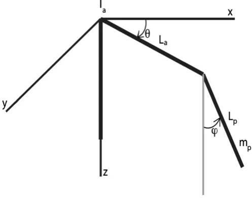
The Furuta pendulum (Furuta, Yamakita, & Kobayashi, 1991; Furuta, Yamakita, Kobayashi, & Nishimura, 1991) has a rotating axle on which a perpendicular arm is fixed from which a pendulum is hinged, as illustrated inFigs. 5and6. Its equations

0 50 100 150 200 250 300 350 400 450 500

[image:7.595.315.559.67.151.2]

−1 0 1 2 3 4 5 6

Fig. 2.Desired (solid) and true (dashed) plant output versus time when the system is controlled by the gain-scheduling controller in (30).

u ˜u

r 1 y

R

−S Σ

T F

[image:7.595.309.564.247.298.2]

Fig. 3.The relation betweenuðtÞ~ andyðtÞis described by the time-varying filter ð1=ð1þFð1=RÞSÞÞF1=R. Hence, by using these signals as input and output in the identification gives us the needed filter directly.

Table 1

The value of the criterion of fitJðrÞfor the initial gain-scheduling controller and after each of two iterations

Iteration # Jðr^Þ

0 0.18

1 0.13

[image:7.595.47.290.536.732.2]

of motion, derived in, e.g.Furuta, Yamakita, and Kobayashi (1991) andBax (2007), are

Ia

y

€þmpl2a

y

€þ14mpl2p

y

€sin

2

_j

þ1₄mpl2p

y

_

j

_sin 2j

1₂mplalp

j

€cosjþ1₂mplalp

j

_2sin

j

þCa

y

_¼M, (32)

Ip

j

€ þ14mpl2p

j

€ 12mplalp

y

€cos

j

18mpl2p

y

_

2

sin 2j

þ1₂mpglpsin

j

þCp

j

_ ¼0, (33)

where the arm angle

y

ðtÞ(rad) and pendulum angle

j

ðtÞ (rad), defined inFig. 5, are functions of timet(s),MðtÞ(Nm) is the torque delivered from the electrical DC-motor,Ia(kg m2) is the moment

of inertia of the axle and arm assembly around its center of mass ,

mp(kg) is the mass of the pendulum with the center of mass at

half length of the pendulum,la(m) is the arm length,lp(m) is the

pendulum length, Ca (Nm/(rad/s)) is the viscous friction

coeffi-cient in the axle joint, Ip (kg m2) is the pendulum moment of

inertia around its center of mass,g(m/s2_{) is the acceleration due}

to gravitation, and Cp (Nm/(rad/s)) is the viscous friction

coefficient of the pendulum joint.Ia,la,lp, andmpare suggested

inFig. 5. Nonlinear effects such as nonlinear friction are neglected.

The rotating axle is driven in an H-bridge configuration by the DC-motor which may be approximated as a current drive for low rotational velocities. HenceMðtÞ kMiðtÞ, wherekM(Nm/A) is the

DC-motor torque constant, andiðtÞis the electrical motor current. Assuming a constant arm rotational velocity

y

_040, such that

2g=ðlp

y

_

2

0Þ¼^dp1, there exist two equilibria with the corresponding

constant driving torque, M0¼

y

_0=Ca, and constant pendulum

angle

j

0 given by cosð

j

0Þ ¼d. Hence, in one equilibrium,

0p

j

0o

p=2, and the pendulum is hanging ‘‘backwards’’ relative

to the motion of the arm, seeFig. 5. It will be shown below that the linearized transfer function around this equilibrium is asymptotically stable, and minimum phase. In the second

equilibrium,

p=2

o

j

0o0, and the pendulum is hanging

‘‘forwards’’ relative to the motion of the arm. The linearized transfer function around the second equilibrium is asymptotically stable, but non-minimum phase. Motions around these equilibria, referred to as the MP case, and NMP case, respectively, will be the subject of this example. Other possible equilibria are investigated in, e.g.,Bax (2007).

The linearized transfer functions around the two equilibria discussed above are

D

j

¼BðsÞ

DðsÞ

D

_

y

with

D

y

_¼DðsÞ

AðsÞ

D

M, (34) where

D

j

¼

j

j

0,

D

y

_¼

y

_

y

_0,

D

M¼MM0, and

BðsÞ ¼mplalpds=2 mpl2p

y

_0d

ffiffiffiffiffiffiffiffiffiffiffiffiffiffi 1d2

q

=2,

DðsÞ ¼ ðIpþmpl2p=4Þs2þCpsþ ðmpglpd=2mpl2p

y

_

2 0ð2d

2

1Þ=4Þ,

AðsÞ ¼ ððIaþmpla2þmpl2pð1d

2

Þ=4ÞðIpþmpl2p=4Þ ðmplalpd=2Þ2Þs3

þ ððIaþmpl2aþmpl2pð1d

2

Þ=4ÞCpþCaðIpþmpl2p=4ÞÞs2

þ ððIaþmpl2aþmpl2pð1d

2

Þ=4Þðmpglpd=2

mpl2p

y

_

2 0ð2d

2

1Þ=4Þ þCaCp

þ ðmpl2p

y

_0d

ffiffiffiffiffiffiffiffiffiffiffiffiffiffi 1d2

q

=2Þ2ÞsþCaðmpglpd=2

mpl2p

y

_

2 0ð2d

2

1Þ=4Þ. (35)

InBðsÞ, the plus sign in front of the constant term belongs to the MP case, and the minus sign to the NMP case. The roots ofDðsÞand

AðsÞare all in the left half of the complex plane for a neighborhood

of the nominal parameter values, Ia¼0:0016, mp¼0:019,

la¼0:33, lp¼0:353, Ca¼0:01, Ip¼0:000789, and Cp¼0:001,

and hence the transfer functions from

D

Mto

D

j, and from

D

y

_ to

0 50 100 150 200 250 300 350 400 450 500

[image:8.595.302.551.68.268.2]

−1 0 1 2 3 4 5 6

Fig. 4.Final tuned gain-scheduling controller: desired (solid) and true (dashed) plant output.

[image:8.595.38.281.70.267.2]

Fig. 5.A sketch of the Furuta pendulum.

[image:8.595.33.282.311.506.2]

D

j

are asymptotically stable. The plant model (32), (33) is nonlinear which makes the transfer functions (34), (35) depend also on the operating point expressed by

y

_0. Hence it could be of

interest to tune a feedback controller for various operating conditions.

The to be controlled measured output signal is the pendulum angle yðtÞ ¼

j

ðtÞ, and the control signal is the motor current

uðtÞ ¼iðtÞ. The reference signal isrðtÞ(rad), and the error is defined as eðtÞ ¼rðtÞ yðtÞ. The criterion to be minimized by controller tuning was chosen as

J¼X

t

e2

ðtÞ=2, (36)

where it is noted thateðtÞandJdepend on the controller and its

parameters, defined below. J is computed over a time interval

when the pendulum exhibits ‘‘steady state’’ behavior, after the passage of the start-up transient. In contrast to the general

criterion in (4) the reference signal is not filtered, and the control effort is not penalized.

The feedback controller was chosen to be a standard PID,

UðsÞ ¼kpð1þ1=tisþ

t

dsÞEðsÞ, whereUðsÞandEðsÞare the Laplace

transforms ofuðtÞ andeðtÞ, respectively, transformed to discrete time form by replacing differentiation with the backward difference:

uðtÞ ¼uðttsÞ þeðtÞkpð1þ

t

d=tsÞ

þeðttsÞkpðts=ti12td=tsÞ þeðt2tsÞkp

t

d=ts, (37)

where t is the sample time (s), and ts¼0:1 s is the sampling

interval. Hence, the parameter vector to be tuned is

r

¼ ½kp;

t

i;

t

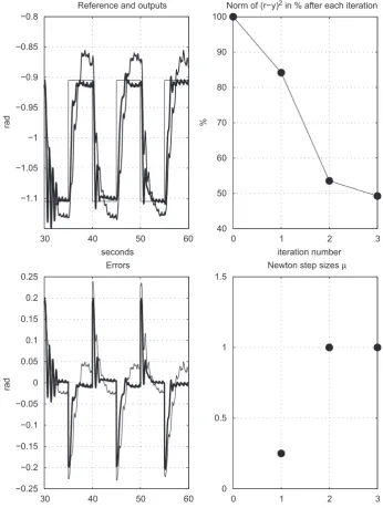
dT. (38)

In the experimental NMP case, the standard Ziegler–Nichols tuning rule was attempted for the initial controller tuning; however, the closed loop became unstable, and the integral action

30 40 50 60

−1.1 −1.05 −1 −0.95 −0.9 −0.85 −0.8

seconds

rad

Reference and outputs

0 1 2 3

40 50 60 70 80 90 100

Norm of (r−y)2 _{in % after each iteration}

iteration number

%

30 40 50 60

−0.25 −0.2 −0.15 −0.1 −0.05 0 0.05 0.1 0.15 0.2 0.25

Errors

seconds

rad

0 1 2 3

0 0.5 1 1.5

Newton step sizes μ

[image:9.595.129.476.265.725.2]

iteration number

had to be weakened. The stabilizing initial controller parameter vector was determined as

r

0¼ ½0:7;2;0:1

T

. SeeFigs. 7and8. An input–output data sequence comprising 1000 samples, i.e., 100 s, was recorded in closed loop, with no extra noise added, since the laboratory equipment ‘‘produced’’ sufficient inherent noise. Following Eq. (31) andFig. 3, a time-varying linear model for the closed loopðTF=RÞ=ð1þSF=RÞfromrðtÞtoyðtÞ, is identified off-line, assuming model (22) withna¼3,nb¼2, andnk¼1. For

each time instant t, the coefficients of A and B in (22) were

obtained by minimizing the weighted least squares criterion

Vða1ðtÞ;. . .;b2ðtÞ;tÞ ¼

1 2

Xn

i¼1

l

jtijðyðiÞ y^ðiÞÞ2 (39)

withn¼1000, the weighting factor

l

¼0:95, andy^ðiÞdenoting the model output. In order to perform the computation in equation (17), the known signalg0 _{is filtered through the identified model}

representingðTF=RÞ=ð1þSF=RÞ, in series with the known filter 1=T, see (11), andy0_{ðtÞis obtained.}

Now an update of

r

takes place according to (6) where the step length

m

is initially chosen to 1, and then decreased by half each time, until criterion (36) decreases. The procedure is iterated with the newly tuned controller as the initial one, until a satisfactory reduction of the criterion is achieved. The final controller

parameter vector was found to be

r

3¼ ½1:4799;11:6068;

0:0045T. The results of this challenging experimental NMP case are illustrated withFigs. 7and8. In this experiment, a reduction of the criterion by 50% is achieved, in three iteration steps, by tuning a standard, but initially quite badly tuned, PID controller.

More simulations and experimental results in both the MP and NMP cases are found inBax (2007). The rate of convergence to a local minimum of the criterion seems to depend on the initial controller tuning, the noise level, and how faithfully the true plant

is modeled. In Bax (2007) a web site is indicated from where

movies of the controlled pendulum can be downloaded.

8. Conclusions

A new algorithm for tuning of controllers of nonlinear systems is presented. The controller parameters are iteratively updated so

that a user-defined control criterion is minimized. In each iteration an experiment on the plant is performed with a specific reference signal. The data from the experiment are used to identify a linearized time-varying model along the reference trajectory, which is then used to calculate the gradient of the control criterion with respect to the control parameters.

Advantages with this approach are

A global nonlinear model of the plant is not needed.

The plant is modeled only where it is necessary—along the

trajectory of the reference signal.

A small simulation example with a tuning of conventionally obtained gain scheduler, and the tuning of a PID controller for a laboratory set-up of the Furuta pendulum are given as illustra-tions of the proposed method.

Acknowledgment

This work has been financed as an ETH-internal project under a special grant approved by ETH research administration. Support from Lady Davis Foundation, Israel and the Swedish Research Council for Engineering Science (TFR), are also gratefully acknowledged.

References

Anderson, B., & Moore, J. (1979).Optimal filtering. Englewood Cliffs, NJ: Prentice-Hall. Astro¨m, K., & Furuta, K. (2000). Swinging up a pendulum by energy control.

Automatica,36(2), 287–295.

Astro¨m, K., & Nilsson, J. (1994). Analysis of a scheme for iterated identification and control. InProceedings of the IFAC symposium on identification(pp. 171–176), Copenhagen, Denmark.

Astro¨m, K., & Wittenmark, B. (1995).Adaptive control (2nd ed.). Reading, MA: Addison-Wesley.

Bax, M. (2007).Implementation of a novel controller tuning algorithm, using linear time varying identification. M.Sc. Report 011CE2007, Control Engineering, EE-Math-CS, University of Twente, The Netherlands, available, including pendulum movies, athwww.mikebax.nli.

Cao, S., Rees, N., & Feng, G. (1997a). Analysis and design for a class of complex control systems, part i.Automatica,33(6), 1017–1028.

Cao, S., Rees, N., & Feng, G. (1997b). Analysis and design for a class of complex control systems, part ii.Automatica,33(6), 1029–1039.

De Bruyne, F., Anderson, B., Gevers, M., & Linard, N. (1997). Iterative controller optimization for nonlinear systems. InProceedings of the IEEE conference on decision and control(pp. 3749–3754), San Diego, USA.

den Hof, P. V., & Schrama, R. (1995). Identification and control—closed loop issues. Automatica,31(12), 1751–1770.

Dennis, J., & Schnabel, R. (1983).Numerical methods for unconstrained optimization and nonlinear equations. Englewood Cliffs, NJ: Prentice-Hall.

Fogel, E., & Huang, Y. (1982). On the value of information in system identifica-tion—bounded noise case.Automatica,18, 229–238.

Furuta, K. (2003). Control of pendulum: From super mechano-system to human adaptive mechatronics. InProceedings of the 42nd IEEE conference on decision and control(Vol. 2, pp. 1498–1507), 9–12 December, Maui, Hawaii, USA. Furuta, K., Yamakita, M., & Kobayashi, S. (1991). Swing up control of inverted

pendulum. InProceedings IECON ’91(Vol. 3, pp. 2193–2198), 28 October–1 November, Kobe, Japan.

Furuta, K., Yamakita, M., Kobayashi, S., & Nishimura, M. (1991). A new inverted pendulum apparatus for education. In N. Kheir, G. Franklin, & M. Rabins (Eds.), Selected papers from the IFAC symposium on advances in control education (pp. 24–25). Boston, MA: Elsevier.

Gevers, M. (1993). Towards a joint design of identification and control? In H. Trentelman, & J. Willems (Eds.),Essay on control: Perspectives in the theory and its applications. Birkhauser.

Gunnarsson, S., & Hjalmarsson, H. (1994).Some aspects of iterative identification and control design schemes. Technical Report, Report LiTH-ISY-1-1653, Department of Electrical Engineering, Linkoping University, Sweden, available by anon-ymous ftp control.isy.liu.se.

Harris, C. (1994).Advances in intelligent control. London: Taylor & Francis Ltd. Hjalmarsson, H., Gevers, M., Gunnarsson, S., & Lequin, O. (1998). Iterative feedback

tuning: Theory and applications.IEEE Control Systems Magazine,18, 26–41. Hjalmarsson, H., Gunnarsson, S., & Gevers, M. (1995). Model-free tuning of a robust

regulator for a flexible transmission system.European Journal on Control,1(2), 148–156.

Horowitz, I. (1982). Feedback systems with nonlinear uncertain plants. Interna-tional Journal of Control,36, 155–171.

40 Bode diagram

30

Gain dB

Phase

20

10

0

-10

10-2 ₁₀-2 ₁₀0 ₁₀1 ₁₀2 ₁₀3

10-2 ₁₀-2 ₁₀0 ₁₀1 ₁₀2 ₁₀3

300

250

200

150

100

50

Frequency (rad/sec)

Frequency (rad/sec)

[image:10.595.33.284.70.291.2]

before after before after

Horowitz, I. (1992).Quantitative feedback design theory (QFT). Boulder, Colorado: QFT Publications.

Hu, J., Kumamaru, K., & Inoue, K. (1996). A hybrid quasi-armax modeling scheme for identification and control of nonlinear systems. InProceedings of the 35th IEEE conference on decision and control(pp. 1413–1418), 11–13 December, Kobe, Japan. Johansen, T., & Foss, B. (1999). Editorial: Multiple model approaches to modelling

and control.International Journal of Control,72(7/8), 575.

Leith, D., & Leithead, W. (2000). Survey of gain-scheduling analysis and design. International Journal of Control,73(11), 1001–1025.

Ljung, L. (1999).System identification: Theory for the user(2nd ed.). Englewood Cliffs, NJ: Prentice-Hall.

Ljung, L., & Soderstrom, T. (1983).Theory and practice of recursive identification. Cambridge, Massachusetts: MIT Press.

Monje, C., Vinagre, B., Feliu, V., & Chen, Y. (2008). Tuning and auto-tuning of fractional order controllers for industry applications. Control Engineering Practice,16(7), 798–812.

Morari, M., & Zafiriou, E. (1989).Process control. Englewood Cliffs, NJ: Prentice-Hall. Murray-Smith, R., & Johansen, T. (1997).Multiple model approaches to modelling and

control. London, UK: Taylor & Francis.

Sjo¨berg, J., & Agarwal, M. (1996). Model-free repetitive control design for nonlinear systems. InProceedings of the 35th conference on decision and control (Vol. 4, pp. 2824–2829), 11–13 December, Kobe, Japan.

Sjo¨berg, J., & Agarwal, M. (1997). Nonlinear controller tuning based on linearized time-variant model. In Proceedings of the American control conference, Albuquerque, New Mexico, 4–6 June.

Sjo¨berg, J., & Agarwal, M. (1998). Tuning neural controllers for trajectory tracking in batch processes. In Proceedings of the 2nd IMACS international multi-conference: CESA’98, computational engineering in systems applications, Ham-mamet, Tunisia.

Sjo¨berg, J., Bruyne, F. D., Agarwal, M., Anderson, B., Gevers, M., Kraus, F., et al. (2003). Iterative controller optimization for nonlinear systems. Control Engineering Practice,11, 1079–1086.

Sjo¨berg, J., Zhang, Q., Ljung, L., Benveniste, A., Deylon, B., Glorennec, P.-Y., et al. (1995). Non-linear black-box modeling in system identification: A unified overview.Automatica,31(12), 1691–1724.

Stark, J. (1999). Delay embeddings for forced systems, part i: Deterministic forcing. Journal of Nonlinear Science,9, 255–332.

Stark, J., Broomhead, D., Davies, M., & Huke, J. (1997). Takens embedding theorems for forced and stochastic systems.Nonlinear Analysis—Theory Methods and Applications,30(8), 5303–5314.

Sternby, J. (1980). Adaptive control of extremum systems. In H. Unbehauen (Ed.), Methods and applications in adaptive control. Proceedings of an international symposium on methods and applications in adaptive control(pp. 151–160). Berlin, Germany: Springer.

Trulsson, E., & Ljung, L. (1985). Adaptive control based on explicit criterion minimization.Automatica,21(4), 385–399.