R E S E A R C H
Open Access
Developing the atlas of cancer in Queensland:
methodological issues
Susanna M Cramb
1,2*, Kerrie L Mengersen
2, Peter D Baade
1,3Abstract
Background:Achieving health equity has been identified as a major challenge, both internationally and within Australia. Inequalities in cancer outcomes are well documented, and must be quantified before they can be addressed. One method of portraying geographical variation in data uses maps. Recently we have produced thematic maps showing the geographical variation in cancer incidence and survival across Queensland, Australia. This article documents the decisions and rationale used in producing these maps, with the aim to assist others in producing chronic disease atlases.
Methods:Bayesian hierarchical models were used to produce the estimates. Justification for the cancers chosen, geographical areas used, modelling method, outcome measures mapped, production of the adjacency matrix, assessment of convergence, sensitivity analyses performed and determination of significant geographical variation is provided.
Conclusions:Although careful consideration of many issues is required, chronic disease atlases are a useful tool for assessing and quantifying geographical inequalities. In addition they help focus research efforts to investigate why the observed inequalities exist, which in turn inform advocacy, policy, support and education programs designed to reduce these inequalities.
Background
Since the 1978 declaration of Alma-Ata which high-lighted the need to address inequalities in health status [1], there have been important advancements for cancer outcomes. Many developed nations have seen improve-ments in cancer survival, notably for colorectal cancer, breast cancer, prostate cancer, non-Hodgkin lymphoma and leukaemia [2,3]. Also, incidence and mortality rates for some cancers have declined [4]. However, notable inequalities in these outcomes persist, with numerous international studies reporting disparities in cancer out-comes across socioeconomic status or urban/rural cate-gories [5-7].
Within Australia, one of the greatest recognised health challenges is achieving health equity for all [8]. Cancer patients living in rural and disadvantaged areas are gen-erally more likely to be diagnosed with advanced cancer and have poorer survival outcomes [9,10]. Often these
areas have a higher prevalence of risk factors such as smoking, obesity and lower levels of physical activity [11,12]. Distance is also important, with cancer patients in rural areas having reduced access to cancer care ser-vices [13-15].
Inequalities need to be quantified before they can be addressed. Maps have been used to portray geographical data for a range of diseases since the mid-1800s, includ-ing cancer [16]. By providinclud-ing a visual representation of cancer outcomes, geographic patterns of disease are able to be identified and effectively addressed [17]. For exam-ple, cancer mortality maps showed high mortality from oral cancer in south-eastern United States of America which led to the identification of snuff dipping as a risk factor [18]. Similarly, mammography screening efforts were intensified after finding low in-situ breast cancer incidence rates from mapped data in north-eastern Con-necticut [19].
We recently developed thematic maps showing the geographical variation in cancer incidence and survival across Queensland, Australia [20]. With a population of 4.2 million [21] and covering an area of 1.9 million * Correspondence: [email protected]
1
Viertel Centre for Research in Cancer Control, Cancer Council Queensland, Gregory Tce, Fortitude Valley, Australia
Full list of author information is available at the end of the article
square kilometres, Queensland has the country’s most decentralized population [22] and the highest incidence of cancer [23]. As there is increasing interest in produ-cing disease maps [24-30], it is hoped that by document-ing the processes and rationale behind the many decisions made during the development of this Cancer Atlas, it may assist others seeking to produce similar types of chronic disease atlases.
Methods
Ethical approval to conduct this study was obtained from the Queensland Health - Central Office Commit-tee Human Research Ethics CommitCommit-tee (HREC/09/ QHC/25). Approval to extract the data was obtained from the Chief Executive Officer - Centre for Health Care Improvement, Queensland Health, under delega-tion by the Director-General, Queensland Health.
Data sources
The Queensland Cancer Registry (QCR) supplied de-identified data on all primary invasive cancers diagnosed among Queensland residents during 1996 to 2007. The QCR is a population-based cancer registry that main-tains a record of all cases of cancer diagnosed in Queensland since 1982, with data currently available to the end of 2007 [31]. Survival status of all cancer patients is obtained through routine linkage with the (Australian) National Death Index, enabling deaths of cancer patients who die interstate to be identified. Across all cancers, 91% of cancers registered by the Queensland Cancer Registry in 2007 were histologically
verified and 1.9% were registered based on death certifi-cate only (DCO) [31]. Cases with unknown age group (0.001% of all cancers) were excluded from the analyses.
Estimated resident population data grouped by age group (0-4, 5-9..., 80-84, 85+), sex, year and statistical local area (SLA) were obtained from the Australian Bureau of Statistics. To calculate the expected popula-tion mortality estimates, de-identified unit record mor-tality data for all causes of death for Queensland residents were also obtained from the Australian Bureau of Statistics (ABS) [32].
Choice of cancers
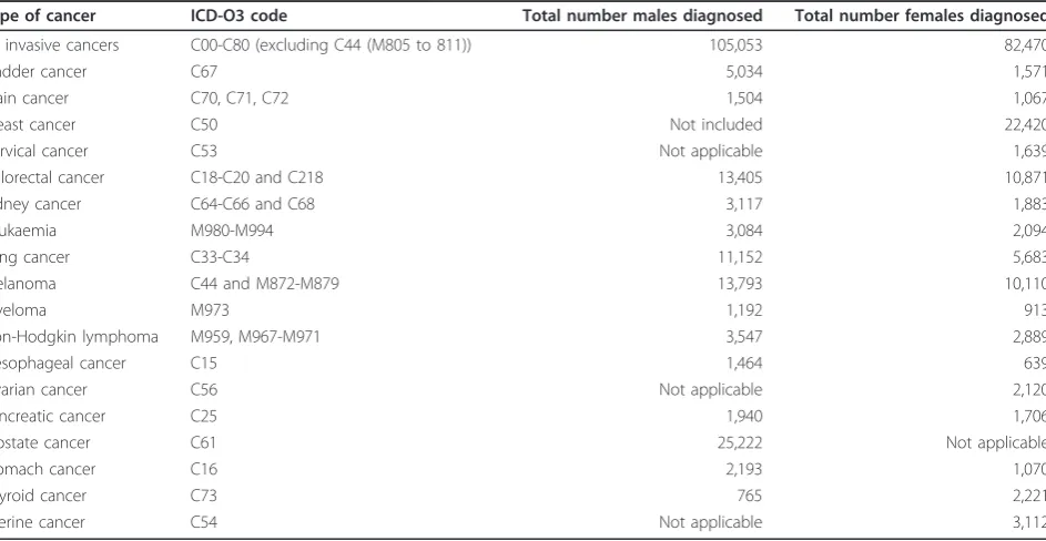
The Cancer Atlas described spatial variation in the lead-ing cancers diagnosed in Queensland durlead-ing the study period (Table 1). These included the (Australian) National Health Priority Area cancers of colorectal can-cer, lung cancan-cer, breast cancan-cer, cervical cancan-cer, prostate cancer and non-Hodgkin’s lymphoma. Although a prior-ity cancer, variation in non-melanocytic skin cancer was not assessed, since it is not routinely reported by popu-lation-based cancer registries in Australia. When a can-cer was not gender specific, results were calculated for each gender. The only exception to this was breast can-cer which was reported for females only due to the very small number of breast cancers diagnosed among males.
Geographical areas
SLAs were used to define the geographical areas. These are part of the Australian Standard Geographic Classifi-cation (ASGC) used by the ABS [33] and are often
Table 1 Cancers examined for geographic variation, Queensland, 1998-2007
Type of cancer ICD-O3 code Total number males diagnosed Total number females diagnosed
All invasive cancers C00-C80 (excluding C44 (M805 to 811)) 105,053 82,470
Bladder cancer C67 5,034 1,571
Brain cancer C70, C71, C72 1,504 1,067
Breast cancer C50 Not included 22,420
Cervical cancer C53 Not applicable 1,639
Colorectal cancer C18-C20 and C218 13,405 10,871
Kidney cancer C64-C66 and C68 3,117 1,883
Leukaemia M980-M994 3,084 2,094
Lung cancer C33-C34 11,152 5,683
Melanoma C44 and M872-M879 13,793 10,110
Myeloma M973 1,192 913
Non-Hodgkin lymphoma M959, M967-M971 3,547 2,889
Oesophageal cancer C15 1,464 639
Ovarian cancer C56 Not applicable 2,120
Pancreatic cancer C25 1,940 1,706
Prostate cancer C61 25,222 Not applicable
Stomach cancer C16 2,193 1,070
Thyroid cancer C73 765 2,221
based on the incorporated bodies of local governments who are responsible for service provision and infrastruc-ture at the local and regional level.
The ABS adjusts the geographical boundaries of SLAs according to changes in the population composition over time. To ensure statistical analyses referred to the same geographical area for the entire study period, all SLAs were mapped to the boundaries used for the 2006 ASGC. The mapping process was conducted within the Queensland Cancer Registry, and matched the suburb and postcode at diagnosis to the 2006 National Local-ities Index [34]. There were 478 SLAs in Queensland in 2006 [33].
Estimates of incidence and survival were also exam-ined by area-level socioeconomic status and rurality. Socioeconomic status was defined using the Socioeco-nomic Indexes for Areas (SEIFA) Index of Relative Socioeconomic Advantage and Disadvantage (IRSAD) compiled by the ABS [35]. Queensland SLAs were ranked from the most disadvantaged to the most advan-taged and then divided into quintiles, based on a variety of data items such as the percentages of: people with high income, people unemployed, households paying cheap rental, households with no car and households with broadband internet connection. Rurality was defined using the ARIA+ (Accessibility/Remoteness Index for Australia plus) classification [36], which defines remoteness on the basis of five categories: major city, inner regional, outer regional, remote and very remote.‘Remote’and‘very remote’categories were com-bined together. The level of remoteness is determined by road-based distance to services.
Methods to generate estimates
To produce a useful map on a small-area scale it is important to have estimates that are robust, or relatively insensitive to outliers, across small areas. If estimates are not robust, these outliers from areas which are often based on very small populations, are more likely to be disproportionately influential, and thus compromise the overall interpretation of the map.
Modelling or smoothing methods are commonly used to generate robust estimates for small geographical areas. As traditional regression models are unable to incorporate spatial correlation, approaches which enable hierarchical structure to be incorporated such as generalised linear mixed models may be used. These may be calculated using either Bayesian, multi-level, or likelihood-based models, however, Bayesian methods do not require the restrictive distributional assumptions in the other models (such as, for example, Gaussian random effects) [37]. Smoothing methods require no distributional assumptions and include interpolation methods, or non-parametric such as kernel regression, kriging and partition methods
[38,39]. They are generally easier and faster to perform than modelling, but a comparison of various modelling and smoothing methods suggested Bayesian models per-formed better than the smoothing methods [40].
Bayesian models incorporate empirical Bayes and fully Bayes methods. In both types of Bayesian models, para-meters are assigned probability distributions, usually based on plausible or expected values, and termed ‘priors’. Fully Bayesian methods assign second stage priors to the variance controlling this distribution (’hyperparameters’). In contrast, empirical Bayes methods estimate the hyperparameter from the distribution of the data [41]. Therefore, empirical Bayes methods give satis-factory point estimates, but are unlikely to provide accu-rate estimates of the associated uncertainty [42].
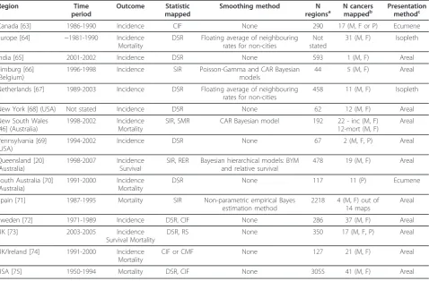
Fully Bayesian models are becoming increasingly com-mon in disease mapping [43]. Advantages of Bayesian models in comparison to other methods include the ease of drawing strength from neighbouring regions so estimates are more reliable and robust, as well as pro-viding better quantification of the uncertainty surround-ing the calculated estimates [41,44]. Also, Bayesian methods enable structuring of more complicated mod-els, inferences and analyses [45]. Other cancer atlases which have used fully Bayesian methods include NSW (Australia) [46] and Limburg (Belgium) [47] (Table 2).
Outcome measures - what to map?
Incidence estimates
Incidence is defined as the number of new invasive can-cer cases diagnosed within a given time period. When examining incidence in small areas, the traditionally used estimate is the SIR (indirectly Standardised Inci-dence Ratio). The SIR is an estimate of relative risk within each area which compares the observed counts against an expected number of counts, based on the population size.
However, limitations associated with the SIR estimates have been previously noted [38]. For example, large dif-ferences can be observed in the SIR estimates even with relatively small changes in incidence counts, and areas with no cases automatically receive an SIR of zero, regardless of the expected counts [40].
average [48]. Alternative measures, such as the Com-parative Incidence Figure (CIF, which is the ratio of the local to national (or whole region) directly standardized rates, i.e. rates weighted by age groups using an external population), have been proposed to overcome this issue, but these have their own disadvantages, including larger standard errors [49]. In light of these evaluations, the modelled SIR was adopted.
Survival estimates
Typically, cancer atlases have tended to report variations in cancer mortality, rather than cancer survival (Table 2). However spatial variations in cancer mortality reflect dif-ferences according to where people die, which may not be where they resided when diagnosed or treated. Mor-tality data are also prone to bias from death certificate inaccuracies in cause of death classification [50]. In con-trast, mapping cancer survival, which is the percentage of
patients who survive for a given time after diagnosis, esti-mates the variation in outcomes based on where people lived when diagnosed. Since treatment generally occurs shortly following diagnosis, this better reflects the poten-tial impact of barriers to treatment and support services.
Survival after the diagnosis of cancer is the most important single measure for monitoring and evaluating the early diagnosis and treatment components of cancer control [51]. When examining cancer survival using population-based data, relative survival is often the pre-ferred method as it provides an estimate of the net can-cer survival without errors from cause of death misclassification, including difficulties in assigning cause of death when cancer was a contributing cause, but may not be completely responsible for the death [52,53].
Relative survival aims to measure deaths in excess of what would be expected, that is, the proportion of
Table 2 Selected Cancer Atlases published from 1995 onwards
Region Time
period
Outcome Statistic mapped
Smoothing method N
regionsa
N cancers mappedb
Presentation methodc
Canada [63] 1986-1990 Incidence CIF None 290 17 (M, F or P) Ecumene
Europe [64] ~1981-1990 Incidence
Mortality
DSR Floating average of neighbouring rates for non-cities
Not stated
31 (M, F) Isopleth
India [65] 2001-2002 Incidence DSR None 593 1 (M, F) Areal
Limburg [66] (Belgium)
1996-1998 Incidence SIR Poisson-Gamma and CAR Bayesian
models
44 5 (M, F) Areal
Netherlands [67] 1989-2003 Incidence DSR Floating average of neighbouring
rates for non-cities
458 11 (M, F) Isopleth
New York [68] (USA) Not stated Incidence DSR None 62 12 (M, F) Areal
New South Wales [46] (Australia)
1998-2002 Incidence
Mortality
SIR, SMR CAR Bayesian model 192 22 - inc (M, F)
12-mort (M, F)
Areal
Pennsylvania [69] (USA)
1994-2002 Incidence DSR None 67 2 (M, F, P) Areal
Queensland [20] (Australia)
1998-2007 Incidence
Survival
SIR, RER Bayesian hierarchical models: BYM and relative survival
478 19 (M, F) Areal
South Australia [70] (Australia)
1991-2000 Incidence
Mortality
DSR None 117 11 (P) Ecumene
Spain [71] 1987-1995 Mortality SIR Non-parametric empirical Bayes
estimation method
2218 4 (M, F) out of 14 maps
Areal
Sweden [72] 1971-1989 Incidence DSR, CIF None 286 37 (M, F) Areal
UK [73] 2003-2005 Incidence
Survival Mortality
DSR, RS None 350 17 (M, F, P) Areal
UK/Ireland [74] 1991-2000 Incidence
Mortality
CIF or CMF None 127 21 (M, F) Areal
USA [75] 1950-1994 Mortality DSR, CIF None 3055 41 (M, F) Areal
a. When multiple areas are available, as for some of the online Atlases, the number of regions is the number at the most detailed level. b. M = males, F = females and P = persons.
c. Ecumene means only populated areas were coloured, Areal indicates that each individual region was coloured, and Isopleth means a continuous gradient was used.
BYM = Besag, York and Mollié CAR = Conditional AutoRegressive.
CIF/CMF = Comparative Incidence/Mortality Figure, and is the ratio of the DSR of the area to the DSR of the entire region or country. DSR = Directly age Standardised Rates.
RER = Relative Excess Risk of death. RS = Relative Survival.
cancer patients alive x years after diagnosis in the hypothetical situation where the cancer in question is the only possible cause of death. Relative survival is modelled via an excess mortality model, which contrasts the mortality in the general population with the mortal-ity of cancer patients. The difference is assumed to be due to cancer-related deaths (’excess mortality’). This model generates the excess hazard, also called relative excess risk (RER).
The median smoothed RER (i.e. exponential of the sum of the spatial and random heterogeneity compo-nents) was mapped. Similar to the interpretation of the SIR, the RER is a comparison against the State average, and comparison between areas is not recommended.
Bayesian hierarchical models
Incidence
For incidence models the Besag, York and Mollié (BYM) model was used, as it has been shown to have desirable properties for disease mapping [43]. This model is
speci-fied as:y e
u v
i i i
i i i
∼Poisson( )
log( )
= + +
where ei is the expected number of cases for theith SLA,θiis the standardised incidence ratio,ais the
over-all level of relative risk, ui is the spatial component modelled with the conditional autoregressive (CAR) prior, andviis the unstructured random effects (which has a normal distribution centered around zero). Input data were aggregated over 1998 to 2007. Since incidence is likely to differ by gender, estimates for males and females were generated separately.
Since this is a fully Bayesian model, priors were speci-fied for a,uiandvi. The prior fora was given a vague normal distribution with mean 0 and variance of 1.0 × 10¹⁰. The prior distributions foruiandvirequired sensi-tivity analyses, and are discussed below.
Relative survival
For relative survival, a recommended approach is to model excess mortality under a generalized linear model based on collapsed data using exact survival times and a Poisson assumption [52]. The basic version of this model was extended to include spatial and random effects, similar to Fairley et al [54].
d
d y u v
kji kji
kji kji kji j k i i
~ ( )
log( * ) log( )
Poisson
x
− = + + + +
Whereykji is person-time at risk in thekth age group, the jth follow up interval and the ith SLA, dkji* is the expected number of deaths due to causes other than the cancer of interest, ajis the intercept (which varied by follow-up year), bk is the coefficient of the predictor
variable vector × (representing the broad age groups),vi is the unstructured random effects (which has a normal distribution) and ui is the spatial component modelled with the CAR prior. Both a andb were given priors with normal distributions having mean 0 and variance 1.0 × 10⁶. The model was run separately for males and females. Broad age groups were included in the model to prevent bias due to differing age structures between SLAs.
All cases considered‘at risk’during 1998 to 2007 were included. Since the earliest year of data was 1996, this meant that any cases diagnosed from 1996 onwards which were alive with up to 5 years follow-up at some stage during 1998-2007 were included. Cases alive on the 31stDecember 2007 were considered censored.
This model excluded persons aged 90 years or older at time of diagnosis, those whose diagnosis was based on death certificate or autopsy only, or those with a survival time of zero days or less. In total, this was 3.3% of the records from 1996-2007.
Adjacency matrix
Since the Bayesian models incorporate information from neighbouring regions, it is necessary to specify the defi-nition of which SLAs are considered neighbours. An adjacency matrix is generated to apply these definitions in the Bayesian model. Using the standard terminology for adjacency options, which follow the possible moves of chess pieces, we used the“Queen”definition, so that SLAs were considered to be neighbours if they shared a common border [55]. The adjacency matrix was calcu-lated using the program GeoDa [56] using 1st order queen adjacencies. Although it is possible to use higher-order weights than first-higher-order (e.g. second-higher-order weights will include neighbours of neighbours), this was not considered useful for this analysis due to the much den-ser neighbourhood matrix and, particularly in rural areas of the state, the very large distances between sec-ond-order neighbouring SLAs.
Due to the large number of island SLAs in Queensland, 18 regions originally had no neighbours. Since estimates will not be smoothed unless a region has neighbours the default neighbourhood matrix was adjusted to ensure all regions had at least one neighbour. Additional neigh-bours were incorporated by considering they could share a border even if separated by a river, or a sea. In particu-lar, most of the Far North islands were grouped together, with some mainland areas also included to ensure enough strength was provided to generate meaningful estimates that were able to converge.
Computation
Thompson, University of Leicester [59]) with a burn-in period of 100,000 iterations (incidence models) and 250,000 iterations (survival models) followed by 100,000 iterations. To decrease the correlation between iterations a subsample of every tenth iteration was kept. Only one chain was run for each estimate.
Assessing convergence
Convergence was assessed using visual examination of trace, density and autocorrelation plots, as well as the Geweke diagnostic [60]. Geweke diagnostics were calcu-lated as the difference between the means for the first 1000 iterations (10%) that were kept and the final 5000 iterations (50%), divided by the asymptotic standard error of the dif-ference. These were generated for the SIR or RER estimates for all 478 SLAs, and any estimate that had a Geweke esti-mate with a p-value of less than 0.01 was considered unli-kely to have converged. To save disk space and processing time, trace and density plots were only generated for 5% (n = 24) of the SLAs, composed of SLAs of concern due to small numbers as well as a random selection.
Sensitivity analyses
For these types of models, and particularly when data are sparse, it is vital to carefully consider the choice of prior and compare the effects of alternate priors. The priors used on the distribution for the variance of the
spatial and random effects components may particularly influence the results.
There were three stages to conducting the sensitivity analyses. First, the literature was searched to determine what priors were being used in similar models. Many BYM models were found, however, there were few examples of Bayesian relative survival models containing spatial components. As there was no other source of information relevant to the study at hand on which to base informative priors, a range of non-informative priors were used for the relative survival models. Sec-ond, the performance of each prior was evaluated. Since the potential influence of the prior will be more pro-nounced for scarce data, Tables 3 and 4 show some of the comparative numbers for a less common cancer -oesophageal cancer in males. In addition to these, observed values were plotted against those predicted by the model and quantile-quantile plots were examined. Third, convergence was examined, as outlined earlier. Lack of convergence could indicate a poor model, or it may simply indicate a longer burn-in period is required. Monitoring the estimate over the entire number of iterations (including burn-in) would show whether it is likely convergence will eventually be reached. In tables 3 and 4 the proportion of SLAs for which the SIR or RER estimate did not converge after discarding 50,000 itera-tions is shown.
Table 3 Sensitivity analyses for oesophageal cancer incidence among males
Prior 1 Prior 2 Prior 3 Prior 4 Prior 5 Prior 6
Distribution of SIR
Mean 100.8 99.4 101.5 100.7 100.6 103.6
Standard deviation 10.2 30.8 16.3 14.5 13.5 23.2
Maximum 140.6 455.1 181.2 169.5 166.4 201.8
75% Quartile 107.2 113.1 111.7 110.2 109.4 109.8
Median 96.5 93.5 95.1 95.6 95.9 95.7
25% Quartile 93.3 78.7 89.4 89.9 90.7 90.2
Minimum 87.4 55.9 79.6 79.3 80.0 79.8
90% ratio1 1.3 2.3 1.6 1.5 1.5 1.6
pD2 34.112 138.047 51.305 53.828 53.709 54.098
DIC3 1652.57 1660.32 1650.62 1648.51 1651.02 1650.71
Spatial fraction4 0.56 0.44 0.63 0.48 0.52 0.57
Percent SLAs with Geweke <0.01 for SIR 41.0% 1.9% 3.3% 9.4% 10.3% 10.5%
Notes:
1. The 90% ratio is calculated as the 95th
percentile divided by the 5th
percentile of the smoothed SIR estimates. 2. pD represents the effective number of parameters in the model. Larger values indicate less smoothing of estimates. 3. DIC = Deviance Information Criterion. Smaller values (of at least 5 below) indicate a better model fit.
4. The spatial fraction estimates the relative contribution of spatial and unstructured heterogeneity, and is calculated as:
Spatial fraction=
+
marginal
marginal 2
2 2
wheremarginal2 = marginal spatial variance,s2
For the sensitivity tests some of the less common can-cers were examined (for incidence: oesophageal, brain, myeloma; for survival (based on number of deaths): oesophageal, thyroid), as well as a more common one (incidence: melanoma; survival: pancreatic).
For both the incidence and survival models, u repre-sents the spatial component, whilevrepresents the ran-dom component. These components were each given hyperprior distributions, as below:
i
i j u i i
N
u u i j N
~ ( )
[ | , , ] ~ ( , )
0 2
2 2
,
≠
where
i j ij
j j ij
i u
j ij
=
=
1
2 2
Σ Σ
Σ
ωij= 1 if SLAs i, jare adjacent (or 0 if they are not).
Theτvalues control the variability ofuandv. As such, the distribution can be specified usingτors, which is the square root of the inverse ofτ(variance =s2).
The following priors were compared for the incidence model:
1. τu ~ Gamma(0.5, 0.0005), τv ~ Gamma(0.5,
0.0005)
2.τu~ Gamma(1,1),τv~ Gamma(7.801, 2.793) 3.τu~ Gamma(0.1, 0.1),τv~ Gamma(0.001, 0.001)
4.τu~ Gamma(0.1, 0.01),τv~ Gamma(0.1, 0.01)
5. Reparameterised ons: su ~ Uniform(0,1), sv ~ Uniform (0,1)
6. Reparameterised ons:su ~ Uniform (0,1000),sv ~ Uniform (0,1000)
Prior 1 shrunk the estimates more than any other (the pD value is lower than the others, and the standard devia-tion smaller) (Table 3). Prior 2 induced far less shrinkage than the others (higher pD and standard deviation). Prior 2 also had a larger DIC (greater than 6 above the others), indicating worse model fit. Priors 3 to 6 gave fairly similar results, although prior 6 had a larger standard deviation.
It was decided to use prior 3 as it provided consis-tently plausible results and converged well across the range of cancers examined.
For the survival model, the following non-informative priors were compared:
1.τu~ Gamma(0.5, 0.001),τv~ Gamma(0.5, 0.001) 2.τu~ Gamma (0.1, 0.1),τv~ Gamma(0.001, 0.001) 3.τu~ Gamma(0.1, 0.01),τv~ Gamma(0.1, 0.01)
4. τu ~ Gamma(0.5, 0.0005), τv ~ Gamma(0.5,
0.0005)
5. Reparameterised ons: su ~ Uniform(0,1), sv ~ Uniform(0,1)
6. Reparameterised ons: su ~ Uniform(0,1000),sv ~ Uniform(0,1000)
Table 4 Sensitivity analyses for oesophageal cancer survival among males
Prior 1 Prior 2 Prior 3 Prior 4 Prior 5 Prior 6
Distribution of RER
Mean 100.2 100.7 100.4 100.1 100.4 100.0
Standard deviation 6.5 11.5 8.2 3.8 9.3 0.3
Maximum 119.6 140.7 127.6 111.3 129.5 102.1
75% Quartile 105.3 105.0 105.7 102.6 106.3 100.2
Median 98.0 97.3 97.7 99.2 97.0 100.0
25% Quartile 95.2 92.6 94.7 97.2 93.7 99.8
Minimum 80.9 63.4 75.0 89.4 72.5 98.3
90% ratio1 1.2 1.4 1.3 1.1 1.3 1.0
pD2 23.988 36.021 33.105 18.663 30.524 18.218
DIC3 3690.23 3690.27 3691.24 3691.32 3690.07 3694.96
Spatial fraction4 0.62 0.87 0.51 0.48 0.80 0.00
Percent SLAs with Geweke <0.01 for RER 89.3% 9.8% 10.5% 19.5% 21.5% 63.0%
Notes:
1. The 90% ratio is calculated as the 95th
percentile divided by the 5th
percentile of the smoothed RER estimates. 2. pD represents the effective number of parameters in the model. Larger values indicate less smoothing of estimates. 3. DIC = Deviance Information Criterion. Smaller values (of at least 5 below) indicate a better model fit.
4. The spatial fraction estimates the relative contribution of spatial and unstructured heterogeneity, and is calculated as:
Spatial fraction=
+
marginal
marginal 2
2 2
Wheremarginal2 = marginal spatial variance,s2
Prior 3 was chosen because it demonstrated greater convergence properties across the range of cancers examined, while restricting the results to a narrower range of smoothed estimates than Prior 2 (Table 4).
Production of maps
A thematic scheme was chosen, with colours determined using color brewer http://colorbrewer2.org under the specifications of a diverging colour-scheme of 5 cate-gories which are suitable for print and colour-blind friendly (Figure 1). The SIRs and RERs were categorised as 10% above and 30% above the State average, and the inverse of these for the lower cut-offs. There is great variability in the categories used in other atlases, but these fairly broad categories were used to reduce the probability of reporting spuriously significant differences.
Mapping alternative measures, such as the posterior probability of exceeding a certain value, were consid-ered, but were deemed unsatisfactory due to difficulties in interpretation and the lack of information provided in regards to the size of the risk [27,44]. Therefore we used graphs to show the precision of the mapped estimates.
Graphs
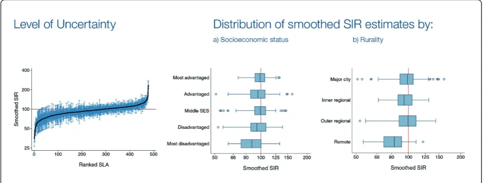
To supplement the information provided in the maps, a graph showing the ranked SIR or RER with the asso-ciated 95% credible interval for each SLA was pro-vided (Figure 2). Horizontal box plots of the SIR or RER estimates by socioeconomic status and rurality were also provided to provide additional information about where the extent of variability across the state (Figure 2). Since a primary purpose of the model was to provide overall estimates of variability across the State, we did not include these additional variables in the model.
Additional data included
For each cancer with significant variation, SIR or RER esti-mates with 95% credible intervals were also provided by socioeconomic and rurality classifications. To calculate these, each iteration of the 10,000 iterations had the mod-elled observed value (incidence) and the adjusted deaths value (survival) calculated as above. For survival (which incorporated age group and time period) these were summed to give 10,000 iterations for each SLA. Each SLA was then grouped into rurality or socioeconomic status
categories, and the adjusted estimates summed. These were divided by the original expected values to produce 10,000 SIR or RER estimates by rurality and socioeco-nomic status categories. The median of these 10,000 was used as the SIR or RER point estimate, and the 2.5 and 97.5 percentiles used to provide the lower and upper cred-ible interval estimates, respectively.
Determining whether observed variation is significant Once the results have been produced and mapped, it is important to determine whether the apparent variation reflects true geographic differences. Therefore, a test for global clustering was conducted. Multiple tests are avail-able [19], such as Besag-Newell’s R, Moran’s I, Oden’s Ipop, but we elected to use Tango’s MEET (Maximised Excess Events Test) [61] as it has been shown to per-form well across a variety of datasets [19].
A small p-value from Tango’s MEET indicates that estimates differ between regions. As is consistent with standard statistical analysis [62], adjusted p-values from the Tango’s MEET statistic below 0.01 were considered to strongly indicate spatial variation, while values between 0.05 and 0.01 were moderately indicative of variation. Values of 0.05 or above were considered to not be significant, however two categories were defined. Values between 0.05 and 0.10 were considered to pro-vide only weak epro-vidence of geographic variation, while values above 0.10 no evidence of geographical variation.
Since Tango’s MEET is calculated using Monte Carlo replications, it is expected that there could be slight var-iations in the results. To increase our confidence that the final classification of geographic variation was stable, Tango’s MEET was run an additional 5 times for each cancer and gender combination. There were only two cases where the final classification did change for
different replication, and so these cancers were assigned to the more conservative, less significant category.
Input for Tango’s MEET requires an observed and expected value. Since the modelled results were of inter-est, the modelled observed value needed to be calculated. For the incidence data, the observed value was calculated by the smoothed SIR median value multiplied by the expected value to produce a modelled observed value. For the relative survival model, the adjusted deaths for each data point were calculated as: (person-time at risk × expfollow-up time× expage group× RER) + expected number of deaths due to causes other than the cancer of interest.
i.e. (ykji×ej ×ek×eui+i)+d*kji
These were then added together for each SLA to pro-vide the input data for Tango’s MEET.
Conclusions
Chronic disease atlases are a useful tool for assessing and quantifying geographical inequalities, as well as assisting to focus research efforts in investigating why the observed inequalities exist. When developing these atlases, a myriad of decisions concerning how to model and present the results need to be made and this paper presents one decision-making algorithm used to gener-ate a cancer atlas.
As with all chronic disease atlases, it is hoped that the presented variations in outcomes will stimulate further research efforts to investigate the reasons underlying the disparities and inform advocacy, policy, support and education programs to effectively address these, so that health equity will become a reality.
The full report is available (from February 2011) at: http://www.cancerqld.org.au/pdf/cancer_atlas.pdf
Author details
1
Viertel Centre for Research in Cancer Control, Cancer Council Queensland, Gregory Tce, Fortitude Valley, Australia.2Centre for Data Analysis, Modelling
and Computation, Queensland University of Technology, George St, Brisbane, Australia.3School of Public Health, Queensland University of
Technology, Herston Rd, Kelvin Grove, Australia.
Authors’contributions
PDB and KLM conceived the study. SMC performed the analysis. SMC and PDB drafted the manuscript. All authors contributed to, read and approved the final manuscript.
Competing interests
The authors declare that they have no competing interests.
Received: 30 September 2010 Accepted: 24 January 2011 Published: 24 January 2011
References
1. World Health Organization:Declaration of Alma-Ata. International Conference
on Primary Health Care, Alma-Ata, USSR, 6-12 September 19781978.
2. Gondos A, Holleczek B, Arndt V, Stegmaier C, Ziegler H, Brenner H:Trends in population-based cancer survival in Germany: to what extent does progress reach older patients?Ann Oncol2007,18:1253-1259.
3. Coleman MP, Gatta G, Verdecchia A, Esteve J, Sant M, Storm H, Allemani C, Ciccolallo L, Santaquilani M, Berrino F:EUROCARE-3 summary: cancer survival in Europe at the end of the 20th century.Ann Oncol2003,
14(Suppl 5):v128-149.
4. National Cancer Institute:Cancer Trends Progress Report - 2009/2010 Update
Bethesda: NCI, NIH, DHHS; 2010.
5. Woods LM, Rachet B, Coleman MP:Origins of socio-economic inequalities in cancer survival: a review.Ann Oncol2006,17:5-19.
6. Wilkinson D, Cameron K:Cancer and cancer risk in South Australia: what evidence for a rural-urban health differential?Aust J Rural Health2004,
12:61-66.
7. Ernst J, Zenger M, Schmidt R, Schwarz R, Brahler E:[Medical and psychosocial care needs of cancer patients: a systematic review comparing urban and rural provisions].Dtsch Med Wochenschr2010,
135:1531-1537.
8. Armstrong BK, Gillespie JA, Leeder SR, Rubin GL, Russell LM:Challenges in health and health care for Australia.Med J Aust2007,187:485-489. 9. Australian Institute of Health and Welfare, Cancer Australia & Australasian
Association of Cancer Registries:Cancer survival and prevalence in Australia:
cancers diagnosed from 1982 to 2004Canberra: AIHW; 2008.
10. Jong KE, Smith DP, Yu XQ, O’Connell DL, Goldstein D, Armstrong BK:
Remoteness of residence and survival from cancer in New South Wales.
Med J Aust2004,180:618-622.
11. Australian Institute of Health and Welfare:A snapshot of men’s health in
regional and remote AustraliaCanberra: AIHW; 2010.
12. Australian Institute of Health and Welfare:Rural, regional and remote
health: indicators of health status and determinants of healthCanberra:
AIHW; 2008.
13. Armstrong K, O’Connell DL, Leong D, D SA, Armstrong BK:The New South
Wales Colorectal Cancer Care Survey Part 1-Surgical ManagementSydney: The
Cancer Council NSW; 2004.
14. Coory MD, Baade PD:Urban-rural differences in prostate cancer mortality, radical prostatectomy and prostate-specific antigen testing in Australia.Med J Aust2005,182:112-115.
15. Kricker A, Haskill J, Armstrong BK:Breast conservation, mastectomy and axillary surgery in New South Wales women in 1992 and 1995.Br J
Cancer2001,85:668-673.
16. Pickle LW:A history and critique of U.S. mortality atlases.Spatial and
Spatio-temporal Epidemiology2009,1:3-17.
17. Lawson AB:Bayesian Disease Mapping: Hierarchical Modeling in Spatial
EpidemiologyBoca Raton: CRC Press; 2008.
18. Mason TJ, McKay FW, Hoover R, Blot WJ, Fraumeni JF:Atlas of cancer
mortality for U.S. counties: 1950-1969Washington: U.S. Govt. Printing Office;
1975.
19. Kulldorff M, Song C, Gregorio D, Samociuk H, DeChello L:Cancer map patterns: are they random or not?Am J Prev Med2006,30:S37-49. 20. Cramb SM, Mengersen KL, Baade PD:Atlas of Cancer in Queensland:
geographical variation in incidence and survival, 1998 to 2007Brisbane:
Viertel Centre for Research in Cancer Control, Cancer Council Queensland; 2011.
21. Australian Bureau of Statistics:3235.0 - Population by Age and Sex, Regions of
Australia, 20072008.
22. Australian Bureau of Statistics:Australian Social Trends 2003Canberra: ABS; 2003.
23. Australian Institute of Health and Welfare, Australasian Association of Cancer Registries:Cancer in Australia: an overview, 2008Canberra: AIHW; 2008.
24. Bhowmick T, Robinson AC, Gruver A, MacEachren AM, Lengerich EJ:
Distributed usability evaluation of the Pennsylvania Cancer Atlas.Int J
Health Geogr2008,7:36.
25. Boulos M:Towards evidence-based, GIS-driven national spatial health information infrastructure and surveillance services in the United Kingdom.International Journal of Health Geographics2004,3:1. 26. Jacquez GM:Current practices in the spatial analysis of cancer: flies in
the ointment.Int J Health Geogr2004,3:22.
27. Bell BS, Hoskins R, Pickle L, Wartenberg D:Current practices in spatial analysis of cancer data: mapping health statistics to inform policymakers and the public.International Journal of Health Geographics2006,5:49. 28. Henry KA, Niu X, Boscoe FP:Geographic disparities in colorectal cancer
survival.Int J Health Geogr2009,8:48.
29. DeChello LM, Sheehan TJ:Spatial analysis of colorectal cancer incidence and proportion of late-stage in Massachusetts residents: 1995-1998.Int J
Health Geogr2007,6:20.
30. Bilancia M, Fedespina A:Geographical clustering of lung cancer in the province of Lecce, Italy: 1992-2001.Int J Health Geogr2009,8:40. 31. Queensland Cancer Registry:Cancer in Queensland: Incidence, Mortality,
Survival and Prevalence,1982 to 2007Brisbane: QCR, Cancer Council
Queensland and Queensland Health; 2010.
32. Australian Bureau of Statistics:Unit record mortality data for Queensland by
State of usual residence, 1982-2007Canberra: ABS; 2009.
33. Australian Bureau of Statistics:Australian Standard Geographic Classification
(ASGC), 2006Canberra: ABS; 2006.
34. Australian Bureau of Statistics:National Localities Index, AustraliaCanberra: ABS; 2007.
35. Australian Bureau of Statistics:Census of Population and Housing:
Socio-Economic Indexes for Areas (SEIFA), Australia, 2006Canberra: ABS; 2008.
36. Glover J, Tennant S:Remote areas statistical geography in Australia: Notes on
the Accessibility/Remoteness Index for Australia (ARIA+ version)Adelaide:
Public Health Information Development Unit, The University of Adelaide; 2003.
37. Waller LA, Gotway CA:Applied spatial statistics for public health dataNew Jersey: Wiley; 2004.
38. Lawson AB, Browne WJ, Vidal Rodeiro CL:Disease mapping with WinBUGS
and MLwiNChichester: John Wiley & Sons Ltd; 2003.
39. Goovaerts P:Geostatistical analysis of disease data: accounting for spatial support and population density in the isopleth mapping of cancer mortality risk using area-to-point Poisson kriging.Int J Health Geogr2006,
5:52.
40. Lawson AB, Biggeri AB, Boehning D, Lesaffre E, Viel JF, Clark A, Schlattmann P, Divino F:Disease mapping models: an empirical evaluation. Disease Mapping Collaborative Group.Stat Med2000,
19:2217-2241.
41. Ghosh M, Natarajan K, Waller LA, Kim D:Hierarchical Bayes GLMs for the analysis of spatial data: An application to disease mapping.Journal of
42. Bernardinelli L, Montomoli C:Empirical Bayes versus fully Bayesian analysis of geographical variation in disease risk.Stat Med1992,
11:983-1007.
43. Best N, Richardson S, Thomson A:A comparison of Bayesian spatial models for disease mapping.Stat Methods Med Res2005,14:35-59. 44. Wakefield J:Disease mapping and spatial regression with count data.
Biostatistics2007,8:158-183.
45. Shen W, Louis TA:Triple-goal estimates for disease mapping.Stat Med
2000,19:2295-2308.
46. Bois JP, Clements MS, Yu XQ, Supramaniam R, Smith DP, Bovaird S, O’Connell DL:Cancer maps for New South Wales 1998 to 2002Sydney: The Cancer Council NSW; 2007.
47. Buntinx F, Geys H, Lousbergh D, Broeders G, Cloes E, Dhollander D, Op De Beeck L, Vanden Brande J, Van Waes A, Molenberghs G:Geographical differences in cancer incidence in the Belgian province of Limburg.Eur J
Cancer2003, ,39:2058-2072.
48. Semenciw RM, Le ND, Marrett LD, Robson DL, Turner D, Walter SD:
Methodological issues in the development of the Canadian Cancer Incidence Atlas.Stat Med2000,19:2437-2449.
49. Breslow N, Day N:The Design and Analysis of Cohort StudiesLyon: International Agency for Research on Cancer; 1987.
50. German RR, Fink AK, Heron M, Stewart SL, Johnson CJ, Finch JL, Yin D:The accuracy of cancer mortality statistics based on death certificates in the United States.Cancer Epidemiol.
51. Dickman PW, Lambert PC, Hakulinen T:Population-based Cancer Survival
AnalysisChichester: Wiley;.
52. Dickman PW, Sloggett A, Hills M, Hakulinen T:Regression models for relative survival.Stat Med2004,23:51-64.
53. Sarfati D, Blakely T, Pearce N:Measuring cancer survival in populations: relative survival vs cancer-specific survival.Int J Epidemiol2010,
39:598-610.
54. Fairley L, Forman D, West R, Manda S:Spatial variation in prostate cancer survival in the Northern and Yorkshire region of England using Bayesian relative survival smoothing.Br J Cancer2008,99:1786-1793.
55. Earnest A, Morgan G, Mengersen K, Ryan L, Summerhayes R, Beard J:
Evaluating the effect of neighbourhood weight matrices on smoothing properties of Conditional Autoregressive (CAR) models.Int J Health Geogr
2007,6:54.
56. Anselin L, Syabri I, Kho Y:GeoDa: An Introduction to Spatial Data Analysis.Geographical Analysis2006,38:5-22.
57. Lunn DJ, Thomas A, Best N, Spiegelhalter DJ:WinBUGS - a Bayesian modelling framework: concepts, structure, and extensibility.Statistics and
Computing2000,10:325-337.
58. StataCorp:Stata Statistical Software: Release 11College Station, TX: StataCorp LP; 2009.
59. Thompson J, Palmer T, Moreno S:Bayesian analysis in Stata using WinBUGS.The Stata Journal2006,6:530-549.
60. Geweke J:Evaluating the accuracy of sampling-based approaches to the calculation of posterior moments.InBayesian Statistics 4.Edited by: Bernardo JM, Berger J, Dawid AP, Smith AFM. Oxford: Oxford University Press; 1992:169-193.
61. Tango T:A test for spatial disease clustering adjusted for multiple testing.Stat Med2000,19:191-204.
62. McPherson G:Applying and Interpreting Statistics: A Comprehensive Guide.2 edition. New York: Springer-Verlag New York Inc; 2001.
63. Le N, Marrett LD, Robson DL, Semenciw RM, Turner D, Walter SD:Canadian
Cancer Incidence AtlasOttawa: Ministry of Supply and Services; 1995.
64. Pukkala E, Söderman B, Okeanov A, Storm H, Rahu M, Hakulinen T, Becker N, Stabenow R, Bjarnadottir K, Stengrevics A, Gurevicius R, Glattre E, Zatonski W, Men T, Barlow L:Cancer atlas of Northern EuropeHelsinki: Cancer Society of Finland; 2001.
65. Nandakumar A, Gupta PC, Gangadharan P, Visweswara RN:Development of
an Atlas of Cancer in India: First all India report 2001-2002Bangalore:
National Cancer Registry Programme (ICMR); 2004.
66. Buntinx F, Cloes E, Dhollander D, Lousbergh D, Op De Beeck L, Rummens JL, Salk E, Vanden Brande J, Van Waes A:Incidence of Cancer in
the Belgian Province of Limburg 1996-1998Hasselt, Diepenbeek, Leuven:
Limburgse Kankerstichting; 2000.
67. Netherlands Cancer Registry cancer incidence maps.[http://www.ikcnet. nl/page.php?id=2487&nav_id=97].
68. New York State Department of Health Maps of Cancer Incidence by County.[http://www.health.state.ny.us/statistics/cancer/registry/cntymaps/ index.htm].
69. Pennsylvania Cancer Atlas: a CDC/GeoVISTA prototype.
[http://www.geovista.psu.edu/grants/CDC].
70. SA Department of Health:The Geography of Cancer in South Australia,1991-2000Adelaide: SA Department of Health; 2005.
71. Benach J, Yasui Y, Borrell C, Rosa E, Pasarín MI, Benach N, Español E, Martínez JM, Daponte A:Atlas of mortality in small areas in Spain
(1987-1995)Barcelona: UPF/MSD; 2001.
72. Swedish Oncological Centres:Atlas of Cancer Incidence in Sweden
Stockholm: Swedish Oncological Centres; 1995.
73. UK Association of Cancer Registries, Association of Public Health Observatories, Cancer Research UK and National Cancer Intelligence Network Cancer e-Atlas.[http://www.ncin.org.uk/cancer_information_tools/ eatlas.aspx].
74. Quinn M, Wood H, Cooper N, Rowan S, Eds:Cancer Atlas of the United Kingdom and Ireland 1991-2000.London: Office for National Statistics; 2005.
75. Devesa SS, Grauman DJ, Blot WJ, Pennello G, Hoover RN, Fraumeni JFJ:
Atlas of cancer mortality in the United States, 1950-94Washington: US Govt
Print Off; 1999.
doi:10.1186/1476-072X-10-9
Cite this article as:Crambet al.:Developing the atlas of cancer in Queensland: methodological issues.International Journal of Health Geographics201110:9.
Submit your next manuscript to BioMed Central and take full advantage of:
• Convenient online submission
• Thorough peer review
• No space constraints or color figure charges
• Immediate publication on acceptance
• Inclusion in PubMed, CAS, Scopus and Google Scholar
• Research which is freely available for redistribution