Doctoral School in Materials Engineering – XXII cycle
M
M
e
e
c
c
h
h
a
a
n
n
i
i
c
c
a
a
l
l
C
C
h
h
a
a
r
r
a
a
c
c
t
t
e
e
r
r
i
i
z
z
a
a
t
t
i
i
o
o
n
n
o
o
f
f
M
M
e
e
t
t
a
a
l
l
l
l
i
i
c
c
M
M
a
a
t
t
e
e
r
r
i
i
a
a
l
l
s
s
b
b
y
y
I
I
n
n
s
s
t
t
r
r
u
u
m
m
e
e
n
n
t
t
e
e
d
d
S
S
p
p
h
h
e
e
r
r
i
i
c
c
a
a
l
l
I
I
n
n
d
d
e
e
n
n
t
t
a
a
t
t
i
i
o
o
n
n
T
T
e
e
s
s
t
t
i
i
n
n
g
g
B
B
e
e
r
r
n
n
a
a
r
r
d
d
o
o
D
D
i
i
s
s
m
m
a
a
M
M
o
o
n
n
e
e
l
l
l
l
i
i
Contents
1 Introduction and overview
PART ONE – STATE OF THE ART
2 Spherical Indentation Mechanics in Elastic-Plastic Solids
2.1 Spherical Indentation Response and Associated Nomenclature
2.1.1 Loading and un-loading indentation depth curves
2.1.2 Crater profile morphologies
2.2 Frictionless Spherical Indentation Stress and Strain Fields in Elastic- Plastic Solids
2.2.1 Indentation Regimes
2.2.2 Hill’s Similarity Solution
2.2.3 Mesarovich and Fleck’s model
2.3 Frictional effects onto the spherical indentation metallic materials response
2.4 Summary
3 Stress-Strain constitutive laws evaluation procedures
3.1 Tabor’s approach
3.2 Modified Tabor’s based approaches
3.3 Evaluation procedures based on the Reference Point Concept
3.3.1 Reference Point Concept
3.3.2 Taljat’s evaluation procedure
3.3.3 Lee’s evaluation procedure
3.4 Evaluation procedures based on the Representative Strain Concept
3.4.1 Representative Strain Concept
3.4.2 Cao’s evaluation procedure
3.4.3 Zhao’s evaluation procedure
3.5 Evaluation procedures based on the Load-Penetration Depth Curve Analysis
3.6 Summary
PART TWO – RESEARCH ACTIVITY
4 Materials and Methods
4.1 Indentation Testing Machine
4.1.1 Technical Specifications and Features
4.1.2 Testing machine Supporting System
4.1.3 Testing machine Indentation Unit
4.1.4 Testing machine zero setting
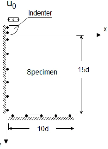
4.2 Computational modelling of the spherical indentation test
4.2.1 Model formulation
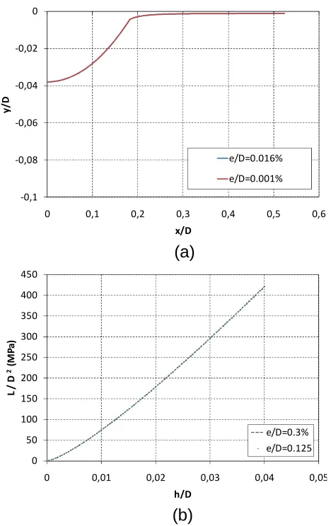
4.2.2 Basic Issues of computational modelling qualification
4.2.3 Mesh density and mesh typology convergence
4.2.4 Indenter compliance and element technology effects
4.3.1 Basic issues of the integration
4.3.2 Experimental constitutive behaviours of the reference materials
4.3.3 Experimental indentation response of the reference materials
4.3.4 Residual crater profile analysis
4.3.5 Testing machine calibration
4.3.6 Computational model validation
4.4 Summary
5 Numerical analysis of the plastic deformation process
5.1 Plastic strains field evolution into the sub-indenter region
5.1.1 Plastic strains field evolution promoted by frictionless indenter
5.1.2 Frictional effects onto the plastic deformation process
5.2 Crater profile evolution
5.2.1 Crater profile evolution in frictionless spherical indentation
5.2.2 Frictional effects onto the crater profile evolution
5.3 Frictional effects onto load – penetration depth curves
5.4 Summary
6 Direct and reverse analysis. Setup and assessment of the algorithms
6.1 Direct analysis
6.1.1 Material model and L-h curves database
6.1.2 L-h curves interpolation
6.2 Reverse Analysis
6.3.1 L-h curve interpolation function
6.3.2 Error analysis
6.3 Experimental validation of the reverse analysis
6.4 Summary
7 Concluding remarks
CHAPTER 1
Introduction and overview
carried out. The research was performed into two steps. The deformation mechanisms promoted by spherical indenters in the sub-indenter region and the procedures developed for inferring the constitutive parameters via analysing the spherical indentation response were investigated in the first part of this dissertation. On the base of the acquired information, a new methodology was built-up in the second part of the present research.
The knowledge of the typical straining phenomena induced by spherical indenters are of paramount importance for understanding which information referring to the behaviour of the indented material are collected by the indentation response. In this frame, Chapter 2 was devoted to review the most prominent indentation theories. Strains field evolution in the sub-indenter region was especially analysed and correlated with the characteristic indentation response represented by the load-indentation depth curve (L-h curve) and crater profile geometry. The evaluation procedures developed to interpret such deformation mechanisms were then focused in Chapter 3. Advantages and drawbacks of each procedure were highlighted.
the reverse analysis for deducing the material parameters from the aforementioned curve were described in Chapter 6.
Finally, interesting topics were presented for future developments.
CHAPTER 2
SPHERICAL INDENTATION MECHANICHS
IN ELASTIC-PLASTIC SOLIDS
The indentation response of any materials is strictly related to the deformation phenomena involved in the region beneath the indenter. Therefore, the constitutive properties evaluation by instrumented indentations testing cannot leave out of consideration a deep understanding of the deformation mechanisms activated by the indenter during the indentation process. Distinguishing and characterizing the straining phenomena induced by the indenter leads to establish which are the material properties and experimental parameters driving the deformation mechanisms and, consequently, how the information concerning the constitutive behaviour of the indented material are collected by the material indentation response. For metallic materials, the indentation response is driven by the elastic-plastic strains field evolution and contact conditions. In the literature there are many theories developed to describe the spherical indentation mechanics, theories based on experimental findings and analytical-numerical approaches.
indentation mechanics of elastic-plastic materials. Special emphasis is dedicated to highlight the limits of each model as well as the agreements with the experimental results in order to establish their accuracy and predictive capabilities. After introducing the main physical quantities, which can be gauged during an instrumented indentation test and the associated nomenclature, the most important experimental findings are reported. Then, the deformation mechanisms promoted by spherical indenters into elastic-ideally plastic and work hardening media are analysed. Correlations with the crater profile evolution and sinking-in and piling-up phenomena are also investigated. Since the friction between the contacting bodies cannot be neglected in the experimental test, frictional effects onto the characteristic load-indentation depth curve and stress-strain fields evolution are also analysed.
2.1 Spherical Indentation Response and Associated
Nomenclature
2.1.1 Loading and un-loading indentation depth curves
only some examples of the large number of applications based on the indentation testing.
As regards to the evaluation of the constitutive laws of metallic materials, instrumented spherical indentation testing is now considered a very attractive tool [27-29]. Fig. 2.1 shows a schematic representation of the spherical indentation test and the attendant load-indentation depth curve (L-h curve) which can be obtained by continuously measuring the driving force L and the indent depth h during the test.
L
h
h L
Figure 2.1. Spherical indentation test and the typical attendant load L – indentation
depth h response of the indented material.
Chen et al. [29] showed that several shape factors characterizing the material indentation response can be recognized by analysing the trends of the loading and unloading curves of the indentation cycle. It is apparent that the maximum applied load Lmax, the corresponding
hmax
Lmax
hres
SC
WL
penetration depth hmax and the residual indentation depth hres must
be considered as the most characteristic parameters of materials indentation response. However, these parameter are not sufficient to uniquely identify the material L-h curve. According to Chen et al. and Chen et al. [27,29], the knowledge of the loading and unloading cycles forms and the areas under these two curves, the total work done by the indenter WL and the elastic work WUN stored in the bulk,
are needed to fully define the frame. In addition, Pharr et al. and Oliver et al. [24,26,30] probed that the initial slope of the unloading curve can be related to the materials elastic properties. Therefore, the slope of the unloading ramp, SC, evaluated at the maximum
reached load can be considered as a further characteristic parameter of the material indentation response.
Experimental findings and analytical predictions [1,31-34] confirm that the form of the loading curve is dictated by the indenter geometry. If sharp indenters are used in the indentation test, the loading cycle is well described by Kick’s Law,
= ℎ (2.1)
where the loading curvature C is a material constant. The quadratic form is an obvious consequence of the geometric indenter self-similarity [31-33].
Conversely, when spherical indenters are driven into the material Meyer’s Law [34-35],
=
⁄
where k and m (>1) are a set of constant depending on the material behaviour, is well-obeyed. Here, D is the diameter of the sphere, whilst a the radius determined by the intersection between the indenter contact profile with the original undeformed surface. As expected, being the self-similarity lost in a spherical indentation test, the corresponding loading curvature C is a function of the penetration depth h and varies during both loading and unloading cycles. However, as shown by O’Neill [36], Meyer’s Law is not just an empiricist relationship between the applied load L and the crater geometry: uniaxial true stress-strain curve of metallic materials, in fact, can be well-fitted by the following power law characterized by the same m exponent,
= ⁄ (2.3)
where τ and γ are Cauchy stress and logarithmic plastic strain, respectively, and κ is a material constant. The extensive analysis by Tabor [1], finally, revealed that k, κ and m are correlated:
= ⁄ (2.4)
and α and β are two universal constants whose values are close to 3.0 and 0.4, respectively. By substituting (2.4) into (2.2), it results,
=
⁄
(2.5)
2.1.1 Crater profile morphologies
Although the material L-h curve represents the primary source of information about the indented material behaviour, the crater profile evolution during the indentation test as well as the residual impression morphology can be used to characterize the material indentation response [37-39]. Typical impression morphologies which can be promoted by indenting a metallic material with a spherical indenter are sketched in Fig. 2.2.
D
aeff
a h heff
D
aeff
a h
heff
Fig. 2.2. Schematic representation of the spherical indentation crater geometry.
Sinking-in (left) and piling-up phenomena (right).
that the actual crater morphology is far from this ideal representation. Material piling-up and sinking-in amounts are related to the indented material constitutive properties [38,39]. Accounting for the real response of the indented surface, the effective indent depth heff,
which represents the actual height of the indenter portion immersed into the indented material, will differ from the penetration depth h. Larger and smaller values of heff with respect to h must be expected if
the material indentation response is governed by piling-up or sinking-in phenomena, respectively. Equally, the actual contact radius aeff will
differ from the surface contact radius “a” and greater or lower values than “a” must result when piling-up and sinking-in phenomena are considered. Accordingly, owing to piling-up and sinking-in phenomena, the effective contact area will be different from the ideal contact area which is obtained if these phenomena are neglected. The extensive body of data elaborated by Norboury et al. [40] also reveals that the penetration depth h can be related to a2 during the indentation process and the ratio,
= /ℎ (2.6)
2.2 Frictionless Spherical Indentation Stress and Strain Fields in
Elastic-Plastic Solids
2.2.1 Indentation Regimes
L-h curve and crater profile evolution during the indentation are a macroscopic effect of the deformation processes occurring in the region beneath the indenter. To establish a proper correlation between the material indentation response and each stage of the indentation process, it is of paramount importance to distinguish the strain processes promoted by spherical indenters as function of material properties and indent depth h.
Figure 2.3. Sketch of the spherical indentation regimen into metallic materials.
Until the yielding stress of the indented material is not exceeded, the strain process is solely driven by the elastic stresses distribution and the elastic contact regime proposed by Hertz [42,43] governs the material indentation response. Accordingly, the load-indent depth curve pertinent to this regime is represented by the well-known power-law found by Hertz [44],
= ∗ℎ ⁄ (2.7)
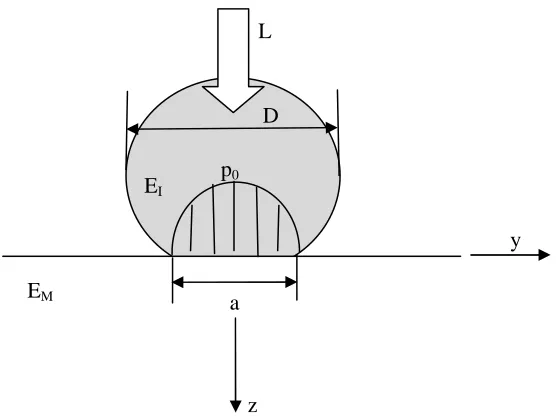
in which the elastic modulus of the indented solid has been replaced by the effective elastic modulus E* defined as ,
"∗= #$"%% +#$"'' (2.8)
z
y D
L
EM
EI
in order to take into account the indenter compliance. Here, EI, *I and
EM, *M represent the Young’s modulus and Poisson ratio of the indenter and indented half-space, respectively. Stress field in the half-space can be derived following the procedure proposed by Timoshenko and Goodier [45], once the loading conditions are known. According to Hertz’s theory, the pressure distribution p(r) between the sphere and the infinite half-space takes the following form:
,-./ = ,0-− ./ ⁄ ⁄ (2.9)
where p0 is the maximum pressure between the contacting bodies.
The equilibrium of the indenter along the indentation axis provides the relationship between the applied load L and p0,
=2,0 (2.10)
Consequently, the elastic stress components on the indented surface
-3 = 0/ and inside the loaded circle -0 ≤ . ≤ / result [45],
67 = 8-#$ '/7 91 − 1 −7
⁄
; − 1 −7 ⁄ < ,0 (2.11a)
6= = − 8-#$'/
7 91 − 1 −
7
⁄
; − 2*?1 −7 ⁄ < ,0 (2.11b)
6@ = − 1 −7
⁄
,0 (2.11c
67 = −6= = -1 − 2*?/7 ,0 (2.12)
Conversely, along the indentation axis (z-axis):
67 = 6= = B−-1 + *?/ C1 −@tan- 3⁄ /#G +1 +@
#
H ,0 (2.13a)
6@ = − 1 +@
#
,0 (2.13b)
It should be noted that along the indentation axis (z-axis) the stress components 67 , 6= and 6@ given by Eqns. (2.13) are principal stresses and the principal shear stress (Fig. 2.4)
= |6@− 6=| (2.14)
takes the maximum value along the indentation axis at a depth
3 = 0.48 for *? = 0.3, as usually occurs for metallic materials.
Therefore, plastic strains development must be expected to initiate in that region beneath the indenter tip centred at the aforementioned depth.
Metallic materials yield is usually well described by either the Von Mises’s Criterion,
NO-6− 6/+ -6− 6/+ -6− 6/P =
QRS
(2.15)
or Tresca’s Criterion,
in which 6, 6 and 6 are the principal stresses and WXY the material yield stress in monotinic uniaxial tension (or compression). By rearranging the Eqns. (2.10), (2.13) and (2.15) or (2.16), it is possible to deduce the plastic onset in terms of the applied load L to the indenter. If QRS denotes the load value at which the plastic deformation process starts to occur, the following relationship among
QRS,indenter geometry and the material yield stress can be obtained:
QRS =
Z
"∗ WXY (2.17)
In terms of indentation average pressure ,, -, = 2⁄ /, the plastic yield onset is achieved when,
, ≈ 1.1WXY (2.18)
response will be affected by both elastic and plastic material properties. As the indentation depth h further increases, it must be expected that the containing effect of the surrounding elastic medium gradually tends to disappear and the plastic strains become dominant. Owing to the loosening of this containing action, the plastic flow can freely spread laterally and break out to the free surface at severe penetration depths, thus entirely surrounding the indenter and producing material piling-up phenomena. It is apparent that the material indentation response at these values of the penetration depths is mainly governed by the plastic properties of the indented material. Slip Line Theory [40,44] can be invoked for determining the transition between the elastic-plastic and fully plastic indentation regimes. According to SLT predictions, the transition to fully plastic indentation regime occurs as the indentation pressure , reaches a value given by the following expression for rigid-plastic solids:
, = WXY (2.19)
where k is a constant depending on the contact conditions (friction coefficient) and the indenter geometry. Its values, however, is approximately equal to 3.0.
engineering materials. However, the expanding spherical cavity model elaborated by Johnson [44,46] may be considered the most effective model for understanding how the strain process proceeds during the elastic-plastic indentation regime and determine the material properties driving the containing action by the surrounding elastic medium. Although the model validity is restricted to linear elastic-ideally plastic solids characterized by a constant yield stress in simple compression, Tabor’s findings [1] have proofed that the expanding cavity model predictions can be extended also to elastic-work hardening solids, thus confirming the general validity of Johnson’s model.
Figure 2.4. Johnson cavity model [44]: iso-strain distribution.
the sub-indenter region as composed by an hemispherical core immediately beneath the indenter having a radius a encased in an annular plastic region. An hydrostatic component of stress ,̅ is assumed to exist in the core, whilst the displacement and stress fields proper of an elastic-ideally plastic spherical cavity under the pressure ,̅ drive the material response outside the core. Let is c
- ≥ / the elastic-plastic boundary radius. Within the plastic zone
- ≤ . ≤ / the stress components are given by Hill [49],
]^
QRS = −2_
`
7 − (2.20a)
]a
QRS = −2_
`
7 + (2.20b)
whereas in the elastic region it results,
]^
QRS = −
`7
(2.21a)
]a
QRS =
` 7 (2.21b)
At the boundary of the core (. = /, (2.20a) leads to
Y̅
QRS = 2_
`
+ (2.22)
neglected, the radial displacement b-./ is given by the following expression:
cd
c7 =
QRS
"'B3-1 − *?/
` 7
− 2-1 − 2*?/ 7`H (2.23)
Compliant indenters may be considered in this analysis by simply replacing the half-space Young’s modulus ? with the elastic modulus ∗ given by Eqn. (2.8). The conservation of core volume leads to
22db-/ = 2dℎ = 2Tan β d (2.24)
for conical indenters, where is the complementary angle of the cone apex semi-angle (Fig. 2.5).
Figure 2.5. Cavity Model for an elastic-plastic indentation by a cone [44].
elastic-plastic boundary c, it is sufficient to substitute . = in Eqn. (2.23), accounting for, that due to the geometrical similarity of cone indenters, during the indentation process d d⁄ = /. It is obtained:
"'lmn o
QRS = 6-1 − *?/
`
− 4-1 − 2*?/ (2.25)
Solving Eqn. (2.25) for and putting the results into Eqn. (2.22), the following expression for the pressure ,̅is obtained:
Y̅ QRS =
B1 + _ q
"'lmn o
QRS rH (2.26)
Eqn (2.26) shows that the pressure ,̅ depends on the non-dimensional variable s ?Tan β W⁄ tXY which may be seen as the ratio between the strain imposed by the indenter -Tan β/ and the elastic strain capacity sWXY⁄ t? offered by the indented material. In other terms, the ratio between the material yield stress and the elastic modulus represents the governing factor of the plastic core evolution in the sub-indenter region during the elastic-plastic regime.
2.2.1 Hill’s Similarity Solution
experimental findings [1,34,36,40]. Therefore, a theory able to explain the observed phenomena is needed.
It should be noted that early experimental results refer to deep indentations, being aimed at evaluating the materials plastic properties. Under these conditions, a direct link between the fully plastic indentation regime and material plastic properties must be addressed.
Unfortunately, SLT [40,44] is only able to establish the transition from the elastic-plastic regime to fully plastic regime. However, as shown by Hill et al. [50], an analytical model able to furnish such correlations can be developed if the following main hypotheses are assumed.
At any stage during the indentation, the indenter causes infinitesimal deformations in the sub-indenter region and the strain path in the sub-indenter infinitesimal volumes is monotonic radial.
Nonlinear elastic behaviour drives the indented material response.
Due to the implications of Hill’s model in the development of the subsequent indentation theories, it is of paramount imporance to review in detail the most important parts of such model. It is evident that the aforementioned hypotheses are very significant from the theoretical point of view. Therefore, the constitutive framework and the effects of these assumptions are firstly delineated.
To begin with, let us denote with 6uv the components of Cauchy stress and with wuvinfinitesimal strain tensor, whilst with xs6uvt and
strictly convex and homogeneous with degres of -_ + 1/ and -T +
1/, respectively. Then,
wuv = zx z6⁄ uv, 6uv = zy zw⁄ uv, wuv6uv = x + y (2.27)
can be treated as the general representation of the elastic response of the indented medium. The Eulero’s identity provides the fundamental connexion,
-_ + 1/x = -T + 1/y = wuv6uv (2.28)
between the potentials. A suitable rearrangement of the Eqn. (2.28) leads to,
x = Ty, y = _x, T_ = 1 (2.29)
Due to the potentials self-similarity, their separate equations can be expressed by positive functions of degree one, as follows:
s6uvt = {|}., swuvt = {|}., (2.30)
whence has the dimension of the stress whilst is a dimensionless parameter. Within this framework, if the potentials are assumed to expressed by the following expressions,
xs6uvt = ~s]t/
-/ , ys6uvt =
~st
-/ (2.31)
= (2.32)
The Eqn. (2.32) proofs how it is possible to derive a constitutive low formally equivalent to that proposed by O’Neill [36] if infinitesimal deformation is assumed to be produced by the indenter in a medium obeying to a nonlinear elastic constitutive law. However, any speculations from now on within this frame and concerning the indentation response of metals cannot be accepted if the equivalence between the metals elasto-plasticity and the constitutive model expressed by the Eqn. (2.32) has been proofed before. In terms of the parameters and the Eqn. (2.27) can be replaced by,
wuv = z z6⁄ uv, 6uv = z zw⁄ uv, wuv6uv = (2.33)
Under the assumption of monotonic radial strain path, the gradients of and remain constant, thus turning out:
wuv = z z6⁄ uv, 6uv = z zw⁄ uv - > 0/ (2.34)
with regards to the incremental response of the indented material. It is apparent that, except for the volume elastic changes, elastic-plastic behaviour of metals is similarly modelled by the relationships (2.34), thus proofing that the nonlinear elastic behaviour can be regarded to model the indentation response of metallic materials in the Meyer’s regime, once the strain path is assumed to be essentially monotonic radial in the sub-indenter region.
wuv = z z6⁄ uv 6uv = z zw⁄ uv wuv6uv = = - ⁄ / (2.35a)
wuv =szbu⁄zUv+zbv⁄ tzUu z6uv⁄zUu = 0 (2.35b)
which must satisfy the following boundary conditions,
6= 6 = 6= 0 -. > / (2.36a)
6= 6 = 0 -. ≤ / (2.36b)
where . = U+ U+ U, whilst the stress field 6uvmust vanish at infinity like 1 .⁄ . Here, bu denote the infinitesimal components of the displacement evaluated at the point Uu. Since the impression profile must be smooth at the contact radius a, an additional conditions relates the contact radius to indent depth h and indenter diameter D. Hence, one of these three parameters or equivalently the ratio ⁄ℎ can be considered an effective eigenvalue, whereas the others two can be regarded as given. The assumed potentials homogeneity, however, ensures the problem self-similarity, i.e. all the solutions of the field problem (2.36), can be generated from just one by an appropriate scaling. In the present case, if the original field variables are uniformly scaled as follow,
Uu = Uu .̃ = . bu = - ⁄ /bu-U, , /
w̃uv = - ⁄ /wuv-U, , / sw̃uvt = - ⁄ /swuvt (2.37)
the driving parameters a, h and D enter into the problem as the ratio
= /ℎ, which is the new expression of the invariant eigenvalue,
thus confirming the early observations of Norboury and Samuel [40]. In addition, due to the invariance, the mean pressure 2⁄ over the contact surface can be evaluated as,
= −
⁄
6-.̃/0 -.̃/ (2.38)
thus proofing that it varies as ⁄ during the indentation process. Accounting for the constitutive framework behind these results, Meyer and O’Neill experimental findings [34,36] can be regarded as successfully modelled by Hill’s theory.
Tabor’s formula may be also included in the present theory. Let us suppose that the integral in the Eqn. (2.38) approximately results equal to ⁄ , where and are two constants only depending on the energy density distribution. Then, from Eqn. (2.38), we would have,
≈
⁄
(2.39)
which is exactly what was found by Tabor [1], after analysing the indentation metal response.
function w(r) the depth below the original surface at a distance r from the indentation axis, then from simple geometry considerations it results:
b-./ = ℎ − ./ -. ≤ / (2.40)
or in terms of scaled variables,
b-.̃/ = 1 ⁄ − . -. ≤ / (2.41)
Thus, the contact perimeter is at a level given by Eqn. (2.41), or equivalently by Eqn. (2.41), and it is below the original surface if
< 1, whilst it is above if > 1. It is now evident how the
parameter governs the sinking-in and piling-up phenomena induced by the spherical indenter. Let is W the total work spent to reach a generic indent depth h and L the corresponding applied load. For frictionless indentation, the total work must be equal to the total strain energy stored by the indented half-space, which is equivalent to the volume integral of yswuvt. In other terms, accounting for the relationship (2.28), W can be evaluated as,
= wuv6uvU = ,-./0 b-./-./ (2.42)
where ,-./ is the contact pressure. The substitution of (2.40) into (2.42) leads to
= ℎ − ,-./
By considering the configuration which must be produced by a spherical indenter, it can easily proofed that,
ℎ = -4_ + 1/ 2_⁄ (2.44)
Finally, by rearranging the relationships (2.43) and (2.44), it can be concluded that
= =# ,-./
0 .-./ (2.45)
which is equivalent to say,
= #
,-.̃/
0 .̃-.̃/ ,-.̃/ 0 .̃-.̃/ (2.46)
if the original variables are replaced by the new scaled variables. Here,
,-.̃/ = - ⁄ / ⁄ ,-.// (2.47)
is the scaled pressure. Eqn. (2.46) allows to appreciate how the material piling-up or sinking-in amounts are related to the strain-hardening coefficient n. Based on an appropriate finite element investigation of nonlinear elastic solids (see Eqn. 2.32), Hill et al. [50] derived the following relationships,
=
#
(2.48)
Matthwes [37] proposed an alternative expression,
=
- /
to fit the data found by Norbury et al. [40].
2.2.1 Mesarovich and Fleck’s model
Although the Hill’s theory is able to model all the most significant experimental findings as well as the role played by the strain-hardening coefficient n in the crater profile evolution during the indentation process, the validity limits of such theory are not established yet. In addition, it should be noted that Hill’s model does not take into account the role of friction onto the material indentation response. Accordingly, a well-established theory able to describe the actual indentation response of metals is not available yet.
It is apparent that, owing to the complexity of the deformation mechanisms promoted by the indenters, the analytical determination of the stress and strain fields evolution as a function of the contact conditions, indent depth and of course of material properties is a challenging essay. It should not be surprising, then, if the major efforts in the comprehension of the indentation phenomena have been spent to built-up numerical models able to simulate the indentation process and interpret their results.
indentation response of infinite half-spaces against which rigid frictionless indenters are driven. As regards to the material constitutive behaviour, homogeneity, isotropy and two constitutive laws, the Hollomon power law,
=
]
], 6 ≤ 60 (2.50a)
=
] ]
, 6 > 60 (2.50b)
and Ramberg-Osgood hardening law,
=
] ]+
] ]
(2.51)
obeying to isotropic J2 flow theory, are considered. Here, 60 and w0 = 60⁄ are the representative strength and corresponding strain of
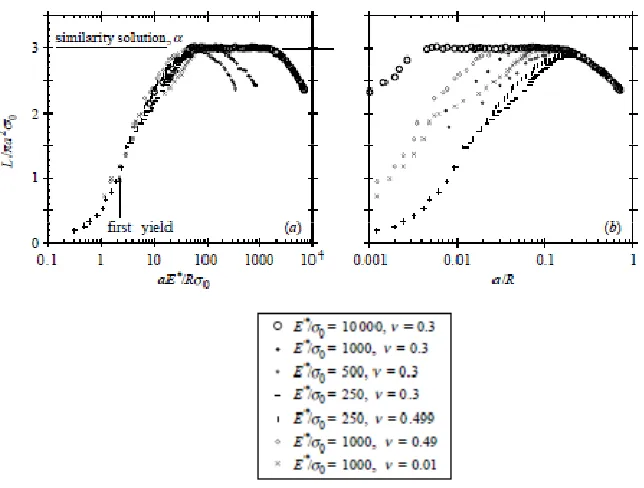
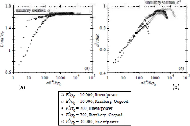
the material respectively, n is the strain-hardening coefficient and ? the corresponding Young’s modulus. In the linear elastic-ideally plastic limit, _ → ∞, the relationships (2.50) and (2.51) are equivalent. To establish the validity limits of the theories previously described and evaluate how they depends on the constitutive properties the main numerical results obtained by Mesarovic and Fleck [54] concerning the frictionless indentation of linear elastic-ideally plastic media can be accounted for (Figure 2.6). The notation of the authors in which R is the sphere radius, a the effective contact radius and h and L respectively the indentation depth and the corresponding applied load to the indenter, is adopted. The results are plotted as a function of the Poisson coefficient *, of the ratio ∗⁄60 (being
and numerical investigations [44,46] suggest that the elastic constant
∗ adequately describes the elastic contribution to the deformation in
the elastic-plastic indentation regime, whereas the amount of deformation are dictated by the ratio between the representative strain ⁄ in the sub-indenter region and the yield strain 60⁄ ∗, thus confirming that the indentation degree depends on the dimensionless parameter ∗⁄-60/. To establish the validity limits of the Hill’s model for linear elastic-ideally plastic constitutive behaviours, the corresponding analytical predictions are also included in Fig. 2.6. The plot of the average pressure against the parameter ∗⁄-60/ reveals that it exist a good agreement between the Hill’s model predictions and the numerical results only for values of the ratio
∗⁄-60/ approximately equal to 40-50. At larger values of this ratio
the average pressure falls down and the normalizing parameter
∗⁄-60/ ceases to uniquely define the amount of the indentation.
Figure 2.6 Frictionless spherical indentation response of linear elastic-ideally
plastic media from [54]: (a) average pressure -2⁄ 60/ as a function of
∗⁄-60/; (b) average pressure as a function o f ⁄ .
especially at points in contact with the indenter surfaces ceases to be infinitesimal and radial.
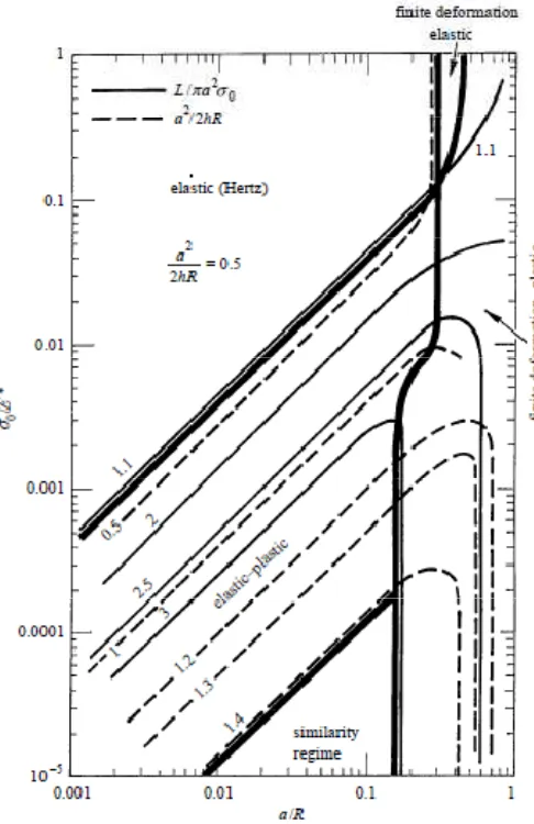
Finally, at very large values of the yield strain -60⁄ ∗ > 0.1/ and contact size ⁄ finite-deformation elastic and plastic regimes dominates the material indentation response.
Figure 2.7. Frictionless spherical indentation response of linear elastic-ideally
plastic media from [54]: indentation map and deformation regimes. The map also
includes the contours of the average pressure (-) and normalized contact area (---).
Figure 2.8. Frictionless spherical indentation response of linear elastic-plastic
hardening solids [54]: (a) average pressure -2⁄ 67/ as a function of ∗⁄-60/
and (b) normalized contact area ⁄-2ℎ/ versus ∗⁄-60/.
The validity limits and the indentation regimes for linear elastic-plastic hardening solids can be better appreciated if the corresponding indentation map is regarded. Fig. 2.9 shows the indentation map of Hollomon materials with _ = 3. For comparison, the indentation map of linear elastic-ideally plastic solids is reported. Overall, the strain hardening coefficient has a barely effects onto the location of the boundaries separating the regimes, especially with regard to the similarity regime: in this case, in fact, the boundaries are mainly determined by the trend of the normalized contact area ⁄-2ℎ/, being the average pressure constant for a wide range of the contact size.
Figure 2.9. Frictionless spherical indentation response of linear elastic-plastic
hardening media with _ = 3 [54]: indentation map and deformation regimes. The
boundaries pertaining the deformation regimes of linear elastic-ideally plastics
solids are included for comparison.
2.3 Frictional effects onto the spherical indentation metallic
materials response
issues [54,55,60], frictional effects onto the material indentation response are not well-established.
Figure 2.10. Frictionless and sticking indentation response of linear elastic-ideally
plastic media with * = 0.3 [54]: (a) average pressure -2⁄ 67/ versus contact size
⁄ ; (b) normalized contact area ⁄-2ℎ/ against ⁄ .
Mesarovic and Fleck [54] investigated the limiting case of sticking friction to establish the sensitivity of the indentation response to the friction level for linear elastic-ideally plastic solids. A comparison of frictionless and sticking indentation is illustrated in Fig. 2.10, for
∗⁄60 = 10 and * = 0.3 , whereas Fig. 2.11 depicts how the
Figure 2.11. Frictionless and sticking indentation response of linear elastic-ideally
plastic media with * = 0.3 [54]: indentation map and deformation regimes.
relatively low yield strengths (i.e. large 6⁄ 0 ratios) and strain-hardening coefficients (small n). For such materials the material piling-up reduces with increasing the friction coefficient - = 0.0 ÷
0.1/. Similar findings were obtained by Habbab et al. [62], after examining material piling-up amount for ratios 6⁄ 0 ranging from 560 and 840 and n between 0.132 and 0.250: crater ridge reductions greater than 50% when friction coefficient increases from 0.0 to 0.5.
Frictional effects onto the L-h curve have been also explored [28,54,55,58,59] via finite element analysis. Although there is not a clear comprehension of friction role from this point of view yet, a trend towards increasing values of the applied load L at a given penetration depth ℎ was found [28,54,58,59]. Conversely, L-h curve seems to be barely affected by friction at low and medium relative indent depths ℎ ⁄ [54,55], whereas it cannot be ignored as the indentation achieves very large values of penetrations depth h. Recently, Cao et al. [59] extended the analysis of frictional effects on L-h curves for deep indentations. Elastic-perfectly plastic materials with 6⁄ 0 in the range 102-2x10³, friction coefficients = 0.0 ÷ 0.3 and relative indentation depths ℎ ⁄ up to 0.15 were considered. An increase of the indentation load L of 28% and 14% at relative penetration depths = 0.15 were observed for materials with 6⁄ 0 equal to 2x10³ and 102 were observed, respectively.
The evaluation of material properties by instrumented spherical indentation testing requires a deep understanding of the deformation mechanisms promoted by the spherical indenter during the test. The present chapter showed that the characteristic indentation response represented by the characteristic L-h curve and the crater geometry impression is strongly related to the achieved indentation depth h and, depending on such variable, different competing indentation regimes can be experienced by the tested material. Under a set of simplifying hypotheses, analytical and numerical approaches proofed that it is possible to establish the driving material parameters governing each indentation regime, thus providing potential guidelines for developing future methodologies for inferring the constitutive laws of the indented materials. The present review also pointed out that friction plays a very important role in the definition of the material indentation response, especially with regard the stress and strain distributions and impression morphology evolution. On the contrary, minor effects seem to be produced in the characteristic load-indent depth curve if no deep penetrations are considered.
limiti principali: leggi constitutive ideali
CHAPTER 3
Stress-Strain constitutive laws evaluation
procedures
The previous chapter allowed to identify the typical response metallic materials to spherical indentation. It also allowed to establishing how and which kind of information coming from the indented material are collected by the indentation response: L-h curve and crater profile evolution. Complex straining mechanisms characterize materials indentation response and many variables affect the experimental data. Accordingly, proper analyses of the materials indentation response are needed to deduce the constitutive properties. Since multiple sources of information can be recognized in the indentation response of any material, different approaches can be adopted for estimating the material behaviour.
procedures based on the analysis of the plastic strain fields in the sub-indenter region and the measured L-h curves are subsequently discussed.
3.1 Tabor’s approach
Although the analysis of the indentation response of metallic materials can be dated back to the XIX century, the first attempt to deduce their constitutive laws was performed by Tabor [1].
Thanks to an extensive analysis of the experimental data, Tabor derived the following relationship,
= 0.2 (3.1)
between the indentation representative plastic strain and the indentation parameters: the indenter diameter and the impression diameter . According to Tabor’s approach, = 2 is the base diameter of the spherical cap impression caused by the indenter, whereas denotes the strain at the contact perimeter between the indenter and indented surface. Therefore, according to this approach, sinking-in and piling-up phenomena are ignored. Following the procedure [1], the corresponding stress is given by:
= (3.2)
introduced to take into account that the effective stress state in the sub-indenter region is unlike to that in the uniaxial tension or compression test [41]. = 3 and the following expression,
= (3.3)
were proposed by Tabor on the base of the experimental data analysis. Eqns. 3.1-3.3 can be used to obtain the true stress – plastic strain curve of the indented material by performing a sequence of loading and unloading cycles, if the contact diameter is known for each value of the load L.
to perform a sequence of loading and unloading cycles, thus preventing any kind of investigation about the constitutive properties of the indented material in a specific points. To avoid potential alterations in the material indentation response, impressions must be carried out at a sufficient distance.
3.2 Modified Tabor’s based approaches
According to the Tabor’s approach, the evaluation of true stress- plastic strain curves is based on the assumption that the constraint factor is fixed and equal to 3. However, on the basis of the analysis of a large amount of experimental results [40,41], it was found that the constraint factor is correlated to the strain-hardening coefficient. The choice = 3 is appropriate only for describing the indentation response of elastic-ideally plastic solids [1]. Francis [68] also proofed that is a function of the indentation regime occurring in the core beneath the indenter and he proposed the following relationship,
= 1.1 + 0.5 log "1.1 2.87
%
" < 1.1 1.1 < " < 27.3
" > 27.3
Hertzian regime Elastic − plastic regime
Fully plastic regime (3.4)
" ==.> ?@9:;< (3.5)
as expression for evaluating ", where
A = BCDE ;E +
BCD
; (3.6)
denotes the reduced modulus. Adopting the notation proposed by Hertz, FB, FG and AB, AG are the Poisson’s ratio and the Young’s moduli of the indented material and the indenter, respectively. Haggag et al. [66,67] modified Francis’s constraint factor and proposed a constraint factor depending on the strain rate and strain hardening,
= 1.12 + H log "1.12 IJ
%
" < 1 1 < " < 27.3
" > 27.3
Hertzian regime Elastic − plastic regime
Fully plastic regime (3.7)
where IJ = 2.87 and H = KIJ − 1.12L/NOK27L.
It is apparent that a more accurate definition of the constraint factor leads to a better estimation of the constitutive law of the indented material.
= P> ;< Q Q<RK G⁄ L
<
RK G⁄ LCQ< T B >⁄
(3.8)
between the aforementioned diameters, where ℎ is the residual crater depth. Conversely, on the basis of an extensive finite element analysis, carried out to explore the material indentation response of elastic-plastic hardening solids, Taljat et al. [65] found that Eqn. (3.8) can be replaced by the following expression,
= VℎK − ℎLWB G⁄ (3.9)
in which ℎ indicates the penetration depth at the load N. Therefore, using Eqn. (3.9), it is possible to deduce the constitutive law of the indented material by a single instrumented indentation test.
determination of the strain-hardening coefficient O and the yielding stress X of materials obeying to the Hollomon power law,
= Y A
XZ ⁄ [X \%
≤ X
> X (3.10)
Here, indicates the total strain (elastic plus plastic), X the strain at yielding onset and A the elastic modulus. The influence of the actual crater geometry onto the stress-strain curve estimation was included by analysing the ratio, ^ = ⁄ , between the effective diameter at the load N and the diameter of the residual impression, as function of the applied load N, the strain-hardening coefficient O and the yielding onset X. To this purpose an extensive Finite Element analysis (FE) was performed and the following power law dependence was finally derived by the authors [56],
^ = ^=ZO, X[N`Z\,?a[ (3.11)
by fitting (via least square method) the FE results over a wide range of values of O and X, Z200 ≤ X ≤ 800, 0.0 ≤ O ≤ 0.5[. Based onto this results, the authors developed an iterative procedure (Fig. 3.1) for deducing the unknowns O and X of metallic materials obeying to the Hollomon power law. After collecting a sequence of b couples
KNc, ℎcL at increasing loads and another sequence b couples
KNc, ℎcL pertaining to the unloading cycle, the effective diameter ,
Figure 3.1. Beghini’s iterative procedure for evaluating the strain-hardening
coefficient O and the yielding stress X of elastic-plastic hardening material
obeying to the Hollomon’s power law [56].
Therefore, putting the results of such computation Eqns. (3.1) to (3.3) and assuming the constraint factor = 2.87, a first estimation of the
no
yes
Applied load-depth couples: Lk −hk or Lk−hpk
Geometrical indentation diameters first approximation: dk(1) (eqn 8)
First approximation σ−ε curve σk(1) (eqn.4) , εk(1) (eqn.1)
Set i=1; regression with eqn (9) for obtaining σy(i)and n(i)
(10) eqn. by diameters physical n Indentatio
dk(i)
) 1 ( curve the of
Points σk i+ (eqn.4) , ) 1 (i+ k
ε (eqn.1)
New evaluation with eqn (9) of σy(i+1) and n(i+1)
Final σ−ε curve
) ( ) 1 ( i y i y σ
σ + ≅
) ( ) 1 (i i
stress-strain curve dQ point can be obtained. Then, using Eqn. (3.9), the unknowns O and X can be computed via least square fitting.These results can be subsequently used for making a better estimation of the effective contact diameter by Eqn. (3.11). Obviously, the iterative procedure is repeated until an appropriate convergence criterion is satisfied.
Although the aforementioned methodologies allow to infer the constitutive properties of any generic metallic material, their validity is strongly limited by the practical difficulty to proof the reliability of the predictions referring to the crater geometry. It is a very difficult task to measure the crater profile left by the indenter. In addition, it should be noted that the afore described procedures do not account for the friction which plays a key role in the evolution of the crater profile [3,13,14].
3.3 Evaluation procedures based on the Reference Point
Concept
3.3.1 Reference Point Concept
able to accurately predict stress-strain curves at large plastic strains is mandatory. Hill et al. and Sinclair et al. [39,68] showed that this limit can be easily overcome, following the Tabor’s approach, by simply changing the point in which the plastic strain is evaluated. Therefore, to infer the constitutive behaviour at large plastic strains, it is sufficient to select a new reference point from which higher values than 0.2 of the plastic strain can be extracted. It is apparent that, changing the reference point, where the plastic strain is evaluated, leads to a new formulation of the constraint factor . Also, new relationships correlating the indentation parameters to the plastic strain are needed. Finally, the definition of new reference points is not straightforward, being the strains distribution into the sub-indenter region affected by the contact conditions which are practically unknown during the test and generally characterized by high gradients [55]. In the next two sections the most powerful and interesting evaluation procedures based on this concept are presented.
3.3.2 Taljat’s evaluation procedure
selected where the plastic strains distribution attains maximum values. Conversely, the second reference point was selected in those regions in which the plastic strain field reaches minimum values, thus making it possible to infer constitutive relationships near the yielding point. In both cases, the selection was performed after exploring the plastic strains distribution beneath the indenter.
Figure 3.2. Taljat’s evaluation procedure [65]: equivalent plastic strain distribution
at the indentation edge for strain-hardening coefficients n between 0.0 and 0.5.
modulus and yield stress of 200 GPa and 400 MPa, respectively. Frictional and indenter compliance effects were also taken into account. Fig. 3.2 summarizes the results obtained by the authors with regard to the trend of the equivalent plastic strain efg at the indentation edge as a function of the normalized distance h ⁄ from the indentation axis ( h denotes the radial distance from the indentation centre). The plotted trends refer to a friction coefficient
i = 0.1. The role played by the strain-hardening coefficient O can be also appreciated.
As shown by the FE results, the equivalent plastic strain efg reaches a maximum value at certain distance from the indentation axis, which is a function of the contact conditions. In the discussed case, maximum values up to 0.6 were attained. Therefore, if the reference point is fixed in this location, it is possible to determine the stress-strain curve up to these values of the plastic stress-strain. By fitting the computed data, the authors established the following relationship,
= P0.5O +√\R=.BB. − 1.6T PT G
(3.12)
between the equivalent plastic strain and the indentation parameters. Since the correlation (3.12) contains the strain-hardening coefficient O, it also accounts for the piling-up and sinking-in phenomena. The constrasinking-int factor dependence on the dimensionless parameter ", the following expression,
= l−0.65 + ln K"L−0.81 + G √\R=.G
%
was finally derived by simply fitting the FE results. A plot of versus
" is shown in Fig. 3.3.
Figure 3.3. Taljat’s evaluation procedure [65]: versus " trends for the
representative stress and strain values at the contact edge and for different values
of the strain-hardening coefficient O.
Following this procedure, the correlations between the plastic strain corresponding to the second reference point and the constraint factor
strain-hardening coefficient O, on the other side, can be derived. According to the authors [] analysis,
= P−2 + 0.87O +√\R=.>nB.m T PTG.oC=.po\ (3.14)
is the correlation correlating to the ratio /, whereas the dependence of on O was found to be given by the following expression:
= K3.65 − 4.30OG+ 4.36O>L PTZC>.Bp\RG.pr\s[ (3.15)
The set of Eqns. (3.12) to (3.15) coupled to Eqns. (3.2) and (3.3) can be used to determine the constitutive behaviour, once a estimation of the strain-hardening coefficient O is provided. Taljat et al. [65] suggested several possibilities for determining this unknown variable: via an appropriate analysis of the L-h curve or by measuring the residual crater profile. More details about this estimation can be found in [17].
between the contacting bodies [39,54,65]. Therefore, it should not be surprising, if the high strain gradients, on one side, and the tangible effects of friction, on the other side, make really hard to have a reliable estimation of stress-strain curves. Moreover, the reference point selection does not take into account the dependence on the penetration depth. As shown by Hill et al., Johnson and Mesarovic and Fleck [39,44,54], the plastic strains distribution varies during the indentation process, thus resulting in a potential modification of the locations where the equivalent plastic strain field takes the maximum or minimum values. Finally, in developing the evaluation procedure, Taljat et al. [65] did not include the variation of the yield strain. The method is valid only for a specific value of the yield strain, thus lacking of practical use.
3.3.3 Lee’s evaluation procedure
Fig. 3.3 illustrates the trends obtained by the authors for the equivalent plastic strain as a function of the normalized distance from the indentation axis K2h ⁄ L and normalized depth Kt ⁄ L under the indented surface.
(a)
(b)
Figure 3.3. Lee’s evaluation procedure [55]: equivalent plastic strain distributions
versus (a) the normalized distance from the indentation axis K2h ⁄ L at a
Both plots refers to the stage K ⁄ L of the indentation process corresponding to the maximum indentation depth.Both plots proofs that trictional effects can be ignored if the reference point location is fixed at a normalized distance 2h ⁄ = 0.8 (Fig. 3.3a) and normalized depth u ⁄ = 0.1 under the indented surface (Fig. 3.3b). At this location, strain gradients are also negligible. This point was selected by Lee et al as new reference point.
Based on these results, Lee et al. [55] developed a novel numerical approach for obtaining automatically the elastic-plastic properties of metallic materials. The constitutive framework is represented by the Hollomon power law,
9 9a= l
X
⁄ Z ⁄ [X \
%
> ≤ X
X, 1 < O ≤∞ (3.16)
in which and X denote the total strain (elastic plus plastic) and the yield strain respectively, whereas X and O the yield stress and the strain-hardening coefficient.
To find the constitutive properties without having recourse to extra processes, as in Taljat et al. and Haggag’s [65-67] indentation theories, the material properties defining the constitutive framework were firstly inter-correlated. To this aim, it is sufficient to note that Eqn. (3.16) can be rearranged as below,
= XZ ⁄ [X B \⁄ = bB \⁄ (3.17)
X = bXB \⁄ (3.18)
whilst the elastic stress-strain relation takes the following form
= AX (3.19)
at the yielding point. Here, A is the Young’s modulus of the indented material. By rearranging Eqns. (3.17) to (3.19), the following inter-correlation between the material properties can be obtained:
= Kb\⁄ LA B K\CBL⁄ = AKb/AL\ K\CBL⁄ (3.20)
The evaluation procedure obviously follows the Tabor’s approach. The actual projected contact diameter at loaded state with pile-up and sink-in,
= 2√ℎ − ℎG = 2vwGℎ − KwGℎLG (3.18)
is evaluated from the geometric shape of the spherical indenter, where ℎ and denotes the actual indentation depth at loaded state and the indenter diameter. ℎ is the nominal depth measured from the original surface.
Such correlations can be easily determined by simulating the spherical indentation process via FE method. The ratio wG = ℎ ℎ⁄ was introduced to evaluate the effects of the yield strain onto the crater geometry.
The dependence of the aforementioned parameters on the yield strain can be determined once the relationships between wG, and
, from one side, and the strain-hardening coefficient O, from the other side, are known. If the Young’s modulus A and yield strength are fixed, the following functional forms can be used,
wG ≡ ℎ ℎ⁄ = iyKℎ⁄ , OL (3.19)
=i\Kℎ⁄ , OL (3.20)
= iKℎ
⁄ , OL (3.21)
for expressing the dependence between wG , and and the indentation parameters and strain-hardening coefficient O . To establish the formulae (3.19) to (3.21), Lee et al. [55] analyzed 13 values of the strain-hardening coefficient O, ranging from 1.001 to 50, and the following relationships,
wG = i
=yKOL + iByKOL ln PQ@T, izyKOL = z{OC{, | = 0,1, } = 0, ,4 (3.22)
= iz9KOL ln PQ@T z
, iz9KOL = ~z{OC{, | = 0, ,3, } = 0, ,4 (3.23)
= izKOL lnKℎ⁄ L z, izKOL = wz{OC{, | = 0, ,3, } = 0, ,4 (3.24)
To establish the relationships between these three characteristic parameters ZwG, , [ and the yield strength X, Lee et al. [55] analysed 364 cases in which the Young’s modulus A and the yielding stress X were considered to vary between 100 GPa and 400 GPa and 200 MPa and 800 MPa, respectively, thus covering a wide range of the engineering materials. In this case the regression of the FE solutions provided the following expressions:
wG = i=yZ
X, O[ + iByZX, O[ lnKℎ⁄ L, izyZX, O[ = z{ZX[OC{,
| = 0,1, } = 0, ,4
z{ZX[ = z{cXc d = 0, ,3 (3.25)
= i=9Z
X, O[ + iB9ZX, O[ lnKℎ⁄ L, iz9ZX, O[ = ~z{ZX[OC{,
| = 0, ,3, } = 0, ,4
~z{ZX[ = z{c=c d = 0, ,3 (3.26)
= i=ZX, O[ + iBZX, O[ lnKℎ⁄ L, izZX, O[ = wz{ZX[OC{,
| = 0, ,3, } = 0, ,4
wz{ZX[ = z{cXc d = 0, ,3 (3.27)
diameter at loaded state for each L-h depth data point on the L-h curve and used to evaluate the values of O, b and X from the stress-strain relationship. The Young’s modulus may be computed following the procedure developed by Oliver et al. or Pharr et al. [24,26,69]. From the analysis of the evaluation procedure developed by Lee et al. [55] three important criticalities emerge: the selection of the reference point, the assessment of the prediction concerning the crater geometry and finally the accuracy of the fitting procedures. The reference point is selected by analyzing the plastic strain distribution when the maximum penetration depth h is attained. However, as shown by Mesarovic and Fleck [54], the size of the region affected by the contact conditions is a function of the penetration depth. Consequently, the choice of the reference point should be also related to the penetration depth. Secondly, due to the difficulties to accurately measure the impression during the experimental indentation test, it is impossible to carry out a validation of the numerically predicted crater profiles. Finally, the presented fitting procedures were performed always on numerical data but it lacks an estimation of the error which these fitting procedures introduce in the final prediction of the material stress-strain curve.
3.4 Evaluation procedures based on the Representative Strain
Concept
The estimation of the material properties via instrumented indentation using the Dimensional Analysis was firstly rationalized by Cheng and Cheng [35,70-72]. Subsequently, Dao et al. [73] applied the dimensional analysis results to introduce the concept of the Representative Strain as a new tool for evaluating stress-strain curves of ductile materials. In both cases, sharp indenters were considered. Cao et al. [58,59] extended the definition of representative strain to spherical indentation and presented new evaluation procedures for obtaining stress-strain curve from the load-indentation depth curve.
Figure 3.4. Hollomon constitutive law. Schematic representation and associated
nomenclature [58].
Although in some cases it may produce a poor description of the materials plastic behavior, the classical Hollomon power law (see Eqn. 3.16) provides a good approximation of the material response, when the yielding onset is exceeded, for many ductile materials. The importance of this constitutive law increases, if it is considered that, as observed by Lee et al. [55] the yielding onset is well defined and only two independent parameters are sufficient to describe the material behavior at these stress states: the yield stress X and the strain-hardening coefficient O.
Adopting this constitutive framework, during the loading cycle of the indentation process and when the yielding occurs, the indentation load L must depend on the following independent parameters only: the Young’s modulus, AB, and the Poisson’s ratio, FB, of the indented material, the Young’s modulus, AG, and the Poisson’s ratio, FG, of the linear-elastic indenter, the yield strength, X, the strain-hardening coefficient, O, the indentation depth, ℎ, and, finally, the indenter radius, . In a functional form:
N = iKAB, FB, AG, FG, X, O, ℎ, L (3.28)
Using the reduced Young’s modulus A∗, Eqn. (3.28) can be rewritten as
N = iKA∗, X, O, ℎ, L (3.29)
= X1 +?a;E \
(3.30)
where in this case indicates the total effective strain accumulated beyond the yield strain X (Fig. 3.4). Let us denote with the flow stress defined at = . As indicated by Eqn. (3.30) is a function of . In terms of , Eqn. (3.29) can be rewritten as
N = iKA∗, , O, ℎ, L (3.31)
where can be computed by Eqn. (3.30). As shown by Barenblatt [74], by applying the theorem, Eqn. (3.31) involving d = 5 independent variables can be equivalently reduced to an equation of
d − dimensioless parameters, being m the number of the fundamental used units. In this case, = 2 and consequently, Eqn. (3.31) takes the following form:
N = ℎGΠBP; ∗
?<, O,QT (3.32)
where the dimensionless function B relates the material indentation response to the material properties, once the indentation depth ℎ and the indenter radius are fixed. It is possible to select a representative stra
![Figure 3.4. Hollomon constitutive law. Schematic representation and associated nomenclature [58]](https://thumb-us.123doks.com/thumbv2/123dok_us/828790.2077886/68.595.206.377.354.503/figure-hollomon-constitutive-law-schematic-representation-associated-nomenclature.webp)
![Figure 4.5. Experimental data analysis system [83]: (a) schematic representation of the experimental load-indentation depth curve measured by the Diaptometro showing the unknown data offset along both coordinate axes and (b) loading curve offset driving pa](https://thumb-us.123doks.com/thumbv2/123dok_us/828790.2077886/95.595.184.414.140.545/experimental-analysis-schematic-representation-experimental-indentation-diaptometro-coordinate.webp)