The Thirty-Third AAAI Conference on Artificial Intelligence (AAAI-19)
A Framework for Approval-Based Budgeting Methods
Nimrod Talmon
Ben-Gurion UniversityBe’er Sheva, Israel [email protected]
Piotr Faliszewski
AGH University Krakow, Poland [email protected]Abstract
We define and study a general framework for approval-based budgeting methods and compare certain methods within this framework by their axiomatic and computational properties. Furthermore, we visualize their behavior on certain Euclidean distributions and analyze them experimentally.
Introduction
Participatory budgeting (Cabannes 2004), initiated by the Brazil workers’ party (Wainwright 2003), is gaining in-creased attention, and is currently applied on many conti-nents, including North America (Gilman 2012) and Europe (e.g., Paris is organizing one of the largest citywide partic-ipatory budgeting processes1). The general premise of par-ticipatory budgeting is to let residents of a municipality in-fluence the way by which their common funds are being distributed, through a deliberative grassroots process. Con-cretely, residents are participating in constructing the mu-nicipal budget, by acting as voters and specifying their pref-erences over a set of available items; then, an aggregation mechanism (i.e., a budgeting method) is applied to decide upon the exact set of items to be funded.
Even though more and more funds are decided through participatory budgets, not many budgeting methods have been proposed, and no mathematical frameworks to allow for a systematic comparison between budgeting methods are available, rendering their use somewhat ad-hoc. Here we de-scribe such a general framework for the approval-based set-ting, in which voters specify subsets of the available items which they approve of. Corresponding methods within our framework differentiate in two aspects: (1) The way by which voter satisfaction from a given set of funded items is defined, modeled through asatisfaction function; and (2) The way these satisfaction functions are used.
We consider several concrete methods within our frame-work, including some which are used in practice and some which generalize known multiwinner voting rules. To com-pare these methods, we (1) consider their computational complexity; (2) define several axioms, relevant to budget-ing methods, and study how well these axioms are satisfied
Copyright c2019, Association for the Advancement of Artificial Intelligence (www.aaai.org). All rights reserved.
1
https://budgetparticipatif.paris.fr/bp
by the methods at hand; and (3) report on three experiments: In the first two, we visualize the behavior of these methods on certain Euclidean preferences, by adapting the methodol-ogy of Elkind et al. (2017a), originally developed for multi-winner voting rules; we are specifically interested in the be-havior of these methods with respect to their preference for choosing either cheap items or expensive ones. In the third experiment we assess how well our budgeting methods deal with local and global items.
The main contributions of our work are: (1) a general framework of approval-based budgeting methods with sev-eral methods within; (2) sevsev-eral useful axiomatic proper-ties which are relevant to budgeting methods at large; (3) an adaptation of the methodology of Elkind et al. (2017a) to participatory budgeting; and (4) an evaluation of certain methods within our framework according to their axiomatic, computational, and visual properties, as well as their ability to deal with local and global items.
Due to space constraints, some proof details are omitted.
Related Work
Researchers have considered ordinal-based budgeting meth-ods, in which voters rank budget items (Goel et al. 2015; Shapiro and Talmon 2017); utility-based budgeting meth-ods, in which voters have numerical utilities over budget items (Fluschnik et al. 2017; Benade et al. 2017); and, as we do, approval-based budgeting methods, in which each voter approves a set of items (Goel et al. 2015; Goel, Kr-ishnaswamy, and Sakshuwong 2016; Benade et al. 2017; Aziz, Lee, and Talmon 2017). Specifically, Goel et al. (2015; 2016) studyk-Approval, where each voter approves exactly
k items, and Knapsack voting, where each voter approves items while respecting the budget limit. As shown below, the aggregation method used by Goel et al., in which the win-ning bundle is selected by greedily considering the items in decreasing number of approvals, fits within our framework.
partic-ipatory budgeting. Their budgeting method, which is a gen-eralization of Phragm´en’s sequential method for committee elections, does not fit within our framework.
As we are interested in axiomatic properties of budget-ing methods, we mention the work of Shapiro and Tal-mon (2017), which considers a generalization of the Con-dorcet principle, the paper of Aziz et al. (2017), which con-siders axioms of representation, and the papers of Fluschnik et al. (2017) and Fain et al. (2018), which also consider representation. Our framework of approval-based budget-ing methods is a generalization of the framework studied by Lackner and Skowron (2017), which regards approval-based multiwinner methods. Our framework, as well as theirs, might be seen as the approval-based variant of the framework of committee scoring rules (Elkind et al. 2017b; Faliszewski et al. 2016b; 2016a). For a general survey of approval-based voting, we point the reader to the work of Laslier and Sanver (2010).
Budgeting Methods
Budgeting Scenarios
We consider the following model of participatory budget-ing. A budgeting scenario E is a tuple E = (A, V, c, `) where A = {a1, . . . , am} is a set of items, c: A → N
is acost function, so that thecostof item a ∈ A isc(a),
V ={v1, . . . , vn}is a set of voters, where each voterv∈V
specifies her approval setAv ⊆ A, containing those items
which she approves of, and`∈Nis a budget limit.
Abudgeting methodRis a function which takes a budget-ing scenarioE = (A, V, c, `)and returns abundleB ⊆A, such that the total cost of the items ofB respects the bud-get limit; i.e., slightly abusing notation, it must hold that
c(B) =P
b∈Bc(b)≤`. The winning bundle (i.e., the set of
funded items) for a budgeting scenarioE, under a budgeting methodR, is denoted byR(E). With respect to a winning bundleB, an item isbudgeted(orfunded) if it is contained inB. For simplicity, we ignore issues related to tie-breaking, which can be dealt with using standard techniques.
Satisfaction Functions
Budgeting methods in our framework operate by consider-ing the satisfaction of the voters from possible bundles. To measure the satisfaction of a voter from a possible winning bundle, we use satisfaction functions, defined below.
Definition 1(Satisfaction function). Asatisfaction function
f is a functionf : 2A×2A→
N, whereAis a set of items.
Given a budgeting scenario with a set of itemsA, a voter
v ∈ V with her approval setAv, and a bundleB ⊆A, the
valuef(Av, B)is thesatisfactionofvfrom the bundleB.
Example 1. Consider a budgeting scenario with A =
{a, b, c}, a voterv withAv = {a, b}, and a bundle B =
{b, c}. For a satisfaction functionf, the valuef(Av, B) =
f({a, b},{b, c})is the satisfaction ofvfrom the bundleB.
Below we give some satisfaction functions. For a bundle
Band a votervwith her approval setAv, letBv :=Av∩B.
1. f(Av, B) =|Bv|: The satisfaction of a voter is the
num-ber of funded items she approves of.
2. f(Av, B) =Pa∈Bvc(a) =c(Bv): A voter’s satisfaction
is the total cost of her approved items which are funded. This follows the intuition that there is some positive cor-relation between the satisfaction of a voter and the funds spent on items approved be her.
3. f(Av, B) = 1|Bv|>0: A voter has satisfaction0if none
of her approved items is funded, and1otherwise (i.e., if at least one of her approved items is funded).
Using Satisfaction Functions
A given satisfaction function can be used in various ways. We consider the following three approaches.
1. Max rules:For a satisfaction functionf, the ruleRm f
se-lects, as a winning bundle, a bundle which maximizes the sum of voters’ satisfaction, according tof. Formally,Rm f
selectsarg maxB⊆AP
v∈V f(Av, B).
2. Greedy rules:For a satisfaction functionf, the ruleRgf
proceeds in iterations, maintaining a partial bundle B, where in each iteration it adds an itematoBwhich maxi-mizes the valueP
v∈V f(Av, B∪{a}). Notice that it halts
only when it is not possible to add more items.
3. Proportional greedy rules:The ruleRpfis similar toRgf, except that in each iteration it adds an itematoBwhich maximizes:
P
v∈V f(Av, B∪ {a})−Pv∈V f(Av, B)
/ c(a).
Remark 1. So, while the Max rules optimally maximize the sum of satisfactions of the voters, the Greedy rules op-erate by greedily maximizing the sum of satisfactions, with-out considering the costs of the items, and the Proportional Greedy rules differ from the Greedy ones in that they oper-ate by greedily maximizing the sum of “satisfaction divided by cost” (i.e., they greedily maximize “bang-per-the-buck”). Example 2. Consider a budgeting scenario with itemsa2,
a3,a4,a5, and a6, where, for 2 ≤ i ≤ 6, item ai costs
i, budget limit ` = 10, and voters v1 = {a2, a5, a6},
v2 = {a2, a3, a4, a5}, v3 = {a3, a4, a5}, v4 = {a4, a5},
andv5={a6}. Then, the winning bundle for this budgeting
scenario underRm
|Bv|is{a2, a3, a5}with total score8, under Rg|B
v|andR
p
|Bv|is{a4, a5}(butR
g
|Bv|selects firsta5and
thena4whileRp|Bv|selectsa4and thena5), underRm1|
Bv|>0
is{a4, a6}which gets the highest total satisfaction possible,
underRg1|
Bv|>0is{a2, a3, a5}(wherea5is selected first and
then perhapsa3anda2, depending on the tie breaking),
un-derRp1|
Bv|>0is{a2, a3, a4}(where firsta2is selected, then
a4, and then perhapsa3, depending on the tie breaking), and
underRm c(Bv),R
g
c(Bv)andR
p
c(Bv)is{a4, a5}.
Remark 2. The above satisfaction functions and approaches result in nine budgeting methods which we discuss through-out the paper. Indeed, studying other functions and ap-proaches is an immediate future work direction. We chose those functions and approaches as they are natural, gen-eralize known multiwinner voting rules, and include some known budgeting methods:Rm
1|Bv|>0 generalizes
Courant 1983; Procaccia, Rosenschein, and Zohar 2008) andRg1
|Bv|>0 generalizes the greedy approximation of this
rule (Lu and Boutilier 2011). Furthermore, Rg|B
v|is
simi-lar to the popusimi-lar k-Approval and Knapsack voting (Goel et al. 2015) (the aggregation method is the same, albeitk -Approval and Knapsack restrict the voter approval sets; we do not consider such restrictions in our framework, as we are interested in the aggregation).
Below, we study the computational and axiomatic proper-ties of our budgeting methods, and report on simulations.
Budgeting Algorithms
We consider the computational complexity of identifying winning bundles. First, it follows from the definitions of the Greedy rules and the Proportional greedy rules that com-puting their winners, given that the functions used can be computed efficiently, can be done in polynomial time; this holds as these rules are defined through efficient iterative processes. This is not the case for Max rules, which in gen-eral are NP-hard. (To be concrete, next we consider a spe-cific Max rule; to be formally correct, we show NP-hardness for deciding whether a bundle with at least a given total sat-isfaction, i.e., sum of satisfaction values, exists.)
Observation 1. Given a budgeting scenario and a bound s, deciding whether a feasible bundleB for which
P
v∈V 1|Bv|>0≥sexists is NP-hard.
Proof. Notice thatRm
1|Bv|>0 generalizes the approval-based
CC rule, which is NP-hard (Procaccia, Rosenschein, and Zohar 2008). Also, when all items are of unit cost, the prob-lem is equivalent to Max Cover (Garey and Johnson 1979; Skowron and Faliszewski 2017).
Next we consider other Max rules. The proof of the next results follows by the similarity of the problem to the Knap-sack problem which is solvable in polynomial-time when-ever one of the dimensions is given in unary.
Proposition 1. Identifying a winning bundle underRm
|Bv|
can be done in polynomial time.
Proposition 2. Identifying winning bundles underRm c(Bv)
can be done in pseudopolynomial time. Further, given a budgeting scenario and a bound s, deciding whether there is a feasible bundle B with P
v∈Vf(Av, B) ≥ s, for
f(Av, B) =Pa∈Bvc(a), is weakly NP-hard.
Proof. Weak NP-hardness follows by a straightforward re-duction from the SUBSETSUMproblem (see, e.g., the text of Garey and Johnson (1979)). Given a Subset Sum instance with integersX = {x1, . . . , xn}, where the existence of a
subsetX0 ⊆ X withP
x∈X0x = Z is to be decided, we construct the following budgeting scenario: For each inte-ger xi, we create a voter vi approving an item ai of cost
c(ai) =xi, and set the limit to be`=Z. For a yes-instance
of Subset Sum, a winning bundle shall be of total cost Z, thus weak NP-hardness follows.
The reduction above also hints on the pseudopolynomial-time algorithm for Rm
c(Bv): Apply dynamic programming
similar to that for Subset Sum, by iterating over the items and remembering the maximum total satisfaction that can be achieved for each amount of money.
Coping with Intractability
We describe a simple Integer Linear Program (ILP) for Max rules over satisfaction functions which can be defined us-ing ILPs; note that all satisfaction functions considered here (i.e.,|Bv|,1|Bv|>0, andc(Bv)) can be defined using ILPs.
This is useful due to the availability of efficient ILP solvers. Indeed, the simulations reported below were performed us-ing the Gurobi ILP solver (Gurobi Optimization 2018) on such ILP formulations.
Observation 2. Letf be a satisfaction function which can be formulated using linear constraints. Then, identifying a winning bundle underRm
f can be done using an ILP.
Next is a general, parameterized complexity result.
Observation 3. For all Max rules, the problem of deciding whether a winning bundle of total cost at least a given value is fixed-parameter tractable for the numbermof items, but there are some Max rules for which this problem is hard even whenn= 1, wherenis the number of voters.
ForRm
c(Bv), which is weakly NP-hard (see Proposition 2)
even when there is only one voter (see the proof of Obser-vation 3), we have a pseudopolynomial time algorithm (see the proof of Proposition 2) and an FPTAS, as we show next.
Observation 4. There is an FPTAS forRm c(Bv).
As forRm
1|Bv|>0, which is NP-hard (see Observation 1),
there is no approximation algorithm with approximation ra-tio better than1−1/e, as it generalizes the multiwinner vot-ing rule CC for approval elections, which itself is equiva-lent to the Max Cover problem (Feige 1998; Skowron and Faliszewski 2017); next we show that it is fixed-parameter tractable for the numbernof the voters.
Proposition 3. Rm
1|Bv|>0is fixed-parameter tractable forn.
Proof. Guess the partition of the voters with the intended meaning that each group of voters in the partition is rep-resented by the same item. For each such group, guess the number of voters which would be satisfied. Then, go over all items and pick as representative the cheapest item that makes exactly this number of voters in this group satisfied.
Budgeting Axioms
In this section we suggest several axiomatic properties which are relevant to budgeting methods. In particular, we focus on axioms which relate to the costs of the items. For each axiom, after providing the definition we check which of the rules in our framework satisfy it. We stress that we view axioms as properties and not necessarily as normative recommendations; thus, while we demonstrate certain situ-ations in which each of the axioms is desirable, there are situations in which failing na axiom is not a drawback.
Rm
|Bv| R
g
|Bv| R
p
|Bv| R
m
1|Bv|>0 R g
1|Bv|>0 R p
1|Bv|>0 R m
c(Bv) R
g
c(Bv) R
p c(Bv)
Complexity P P P NP-h P P weak NP-h P P
Inclusion Maximality X X X X X X X X X
Discount Monotonicity X X X X X X x x x
Splitting Monotonicity X X X X X X X x X
Merging Monotonicity x x x X X x X X X
Limit Monotonicity x x x x x x x x x
Table 1: Computational and axiomatic properties of certain approval-based budgeting methods.
x Rm
|Bv| R
g
|Bv| R
p
|Bv| R
m
1|Bv|>0 R
g
1|Bv|>0 R
p
1|Bv|>0 R
m
c(Bv) R
g
c(Bv) R
p c(Bv)
10
30
90
190
Table 2: Results of Experiment1. Cheap items are on the left, expensive on the right.
items, then we should; i.e., voters might wish to use all the available funds. Formally, we express it as follows.
Definition 2 (Inclusion Maximality). A budgeting method R satisfies Inclusion Maximality if for each budgeting scenario E = (A, V, c, `) and each pair of feasible bundlesBandB0 such thatB ⊂B0 it holds that if
Bis winning then alsoB0is winning.
Inclusion Maximality seems desirable in all cases of par-ticipatory budgeting. Yet, a somewhat artificial example shows that not all rules in our framework satisfy it.
Example 3. Letf(Av, B) = min({c(a) :a ∈ Bv}); that
is, the satisfaction of a voter equals the cost of her cheapest approved item which is funded. Then,Rm
f does not satisfy
Inclusion Maximality (to see it, consider two itemsa,bof cost1,2respectively, one voter approving bothaandb, and a pair of bundlesB ={b}andB0={b, a}).
Nevertheless, notice that all three satisfaction functions we consider here (namelyf =|Bv|,f =1|Bv|>0, andf = c(Bv)) are super-set monotone; that is, for each of them, we
have thatf(B0)≥f(B)for eachB ⊂B0. Thus, since one can verify that Max rules are Inclusion Maximal for super-set monotone satisfaction functions, we have the following. Corollary 1. Rm
|Bv|, R
m
c(Bv), and R
m
1|Bv|>0, satisfy
Inclu-sion Maximality.
For Greedy rules and Proportional greedy rules, it is never the case that two feasible bundlesB,B0 withB ⊂B0 are both winning, so we have the following.
Corollary 2. Rg|B v|,R
g c(Bv),R
g
1|Bv|>0,R p
|Bv|,R
p
c(Bv), and Rp1
|Bv|>0, satisfy Inclusion Maximality.
In the next axiom we consider the response of our rules to increasing the available budget limit. Specifically, we quire that if we increase the limit, then all funded items re-main funded, provided that no new item becomes affordable (this last condidtion is quite natural; if there is an item that all the voters approve, which is above the budget limit before its extension but is within the limit after the extension, then it is quite natural that this item might be funded and might remove many previously funded ones).
Definition 3(Limit Monotonicity). We say that a budgeting methodR satisfies Limit Monotonicity if for each pair of budgeting scenariosE= (A, V, c, `),E0 = (A, V, c, `+ 1) with no item which costs exactly`+ 1, for eacha∈ A, it holds thata∈ R(E) =⇒ a∈ R(E0).
Interestingly, while Limit Monotonicity generalizes the Committee Monotonicity axiom of multiwinner voting rules (Elkind et al. 2017b), which is satisfied by many such rules, Limit Monotinicity is not satisfied by any of the rules we consider here. This shows that even though the frame-works of participatory budgeting and multiwinner voting are strongly related, the fact that the former deals with items of different costs can lead to significant differences.
Proposition 4. None ofRm
|Bv|,R
m
c(Bv), andR
m
1|Bv|>0
x Rm
|Bv| R
g
|Bv| R
p
|Bv| R
m
1|Bv|>0 R
g
1|Bv|>0 R
p
1|Bv|>0 R
m
c(Bv) R
g
c(Bv) R
p c(Bv)
0
10
50
70
100
Table 3: Results of Experiment2. Cheap items are on the left, expensive on the right.
Proof. Below we consider each of the three rules separately.
Rm
1|Bv|>0:Consider a budgeting scenarioE with itemsa, b, and c, all of unit cost, and four voters: v1 : {a}; v2 :
{a, b}; v3 : {b, c}; v4 : {c}. Then, with budget limit 1 a
winning bundle might be{b}, while with budget limit2the only winning bundle is{a, c}.
Rm
c(Bv):Consider a budgeting scenarioEwith itemsa,b,c, andd, with costs2,3,3, and5, respectively, and one voter:
v1 :{a, b, c, d}. Then, with budget limit6the only winning
bundle is{b, c}, while with budget limit7the only winning bundle is{a, d}.
Rm
|Bv|: Consider a budgeting scenario E with the same items as above and five voters: v1 : {a, b, c, d}; v2 :
{a, b, c, d}; v3 : {b, c, d};v4 : {d}; v5 : {d}. Then, with
budget limit6the only winning bundle is{b, c}, while with budget limit7the only winning bundle is{a, d}.
Greedy and Proportional greedy rules also fail Limit Monotonicity. Consider a budgeting scenario with itemsa,b, andc, whereahas the largest value according to the relevant satisfaction function; thus,ais selected in the first iteration. Set the cost ofaso that, after selecting it, the remaining bud-get limit is such that, for the original budbud-get limit`, onlyb
can be selected, while for the budget limit`+ 1, alsoccan be selected. Set the value of cto be higher than that of b. Thus,bis selected in the first case andcin the second case.
Corollary 3. Rg|B v|,R
g c(Bv),R
g
1|Bv|>0,R p
|Bv|,R
p
c(Bv), and Rp1|
Bv|>0, do not satisfy Limit Monotonicity.
As neither of our rules satisfies Limit Monotonicity, it is natural to wonder if the axiom is truly useful. One argument in its favor is that it would be surprising for voters to learn that due to increasing the available funds their approved item
ceases to be funded. Thus if one uses a budgeting method that fails Limit Monotonicity then one should make sure that the budget is fixed ahead of voting and is neither increased nor decreased later (as it leads to suspicion of manipulation). A budgeting methodRsatisfies Discount Monotonicity if any funded item remains funded when its price decreases. This is a very desirable property as failing it means that peo-ple proposing new items for the participatory budget have to think strategically about the item’s price, instead of trying to minimize it.
Definition 4(Discount Monotonicity). A budgeting method
Rsatisfies Discount Monotonicity if for each budgeting sce-nario E = (A, V, c, `) and for each b ∈ R(E), it holds thatb ∈ R(E0)forE0 = (A, V, c0, `), where for each item
a ∈ A, we have that c0(a) = c(a)whenever a 6= b, and
c0(b) =c(b)−1.
Proposition 5. Rm
|Bv|,R
m
1|Bv|>0,R g
|Bv|,R
g
1|Bv|>0,R p
|Bv|,
andRp1|
Bv|>0, satisfy Discount Monotonicity, whileR m c(Bv), Rgc(B
v), andR
p
c(Bv)fail it.
Proof sketch. Intuitively, forf = |Bv| andf = 1|Bv|>0,
decreasing the cost only increases the attractiveness of the item, while forf = c(Bv), decreasing the cost makes the
item less attractive.
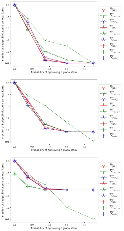
Table 4: Results of Experiment3. The top, middle, and bot-tom figure are for`= 20,30, and50, respectively.
Definition 5(Splitting Monotonicity). A budgeting method
Rsatisfies Splitting Monotonicity if for each budgeting sce-narioE = (A, V, c, `), for eacha ∈ R(E), and for each budgeting scenarioE0 which is formed by splittingainto a set of items A0 with c(a) = c(A0), and such that the voters which approve a in E approve all items of A0 in
E0 and no other voters approve items ofA0, it holds that
R(E0)∩A0 6=∅.
Remark 3. Note that in the above definition we assume that if a voter approves an item, then this voter also approves all the projects that result from splitting it. While in some cases this is true (e.g., when the voters recognize that several items form a larger project), in some others it would be false (e.g., when voters decide that completing only a part of a larger project is sufficient and remaining funds should be used for other purposes). In practice we expect both types of behavior to occur and it would be natural to study variants
of Splitting Monotonicity that take such more complicated behaviors into account.
Proposition 6. Rm
|Bv|,R
m
1|Bv|>0,R g
|Bv|,R
g
1|Bv|>0,R p
|Bv|, Rp1
|Bv|>0,R m
c(Bv), andR
p
c(Bv), satisfy Splitting
Monotonic-ity, whileRgc(B
v)does not satisfy Splitting Monotonicity.
Proof sketch. Intuitively,Rgc(B
v) does not satisfy Splitting
Monotonicity as the new items’ value is less than the original item’s value. For other rules, the new items’ value is at least as the original item’s value, thus at least one is selected.
Definition 6 (Merging Monotonicity). A budgeting method R satisfies Merging Monotonicity if for each budgeting scenario E = (V, A, c, `), and for each
A0 ⊆ R(E) such that for each v ∈ V we either have
v ∩A0 = ∅ or A0 ⊆ Av, it holds that a ∈ R(E0) for
E0 = (A\A0 ∪ {a}, V0, c0, `),c0(a) = P
a∈A0c(a), and each voter v ∈ V for which A0 ⊆ Av in E, approves a
inE0, and no other voter approvesa.
Proposition 7. Rm
1|Bv|>0, R m c(Bv),R
g
1|Bv|>0, R g
c(Bv), and Rpc(B
v), satisfy Merging Monotonicity, while R
p
1|Bv|>0,
Rm
|Bv|,R
g
|Bv|, andR
p
|Bv|fail it.
Proof sketch. Intuitively, for the satisfaction function
f(Av, B) =|Bv|, the value of the original items decreases
but the merged item is as expensive. Forf(Av, B) =c(Bv),
the value of the merged item equals the total value of the merged items. Forf(Av, B) =1|Bv|>0the fact that all the
original items were funded means that the merged item still satisfies the same voters.
As in the case of Discount Monotonicity, the main advan-tage of rules satisfying Splitting and Merging Monotonicity axioms is that it reduces the need for strategic thinking on the part of the project proposers.
Experiments on Budgeting Methods
In this section we report on three experiments: Two experi-ments generalize the technique of Elkind et al. (2017a), used quite extensively for multiwinner elections (Faliszewski, Sz-ufa, and Talmon 2018; Aziz et al. 2018; Faliszewski and Tal-mon 2018), to the setting of approval-based budgeting sce-narios. One experiment focuses on locality issues, assuming certain projects are more relevant to certain voters and others are relevant to all.For the first two experiments, for each particular sim-ulation setting we generate several corresponding budget-ing scenarios by samplbudget-ing from these distributions, compute the winning bundle in each of them, and aggregate the re-sults into a2-dimensional histogram. These histograms are formed by first partitioning the square from(0,0)to(1,1) into bins (we use50×50bins). Then, we draw a pixel in each of these bins, where the more funds spent on this bin, the brighter the pixel is drawn. Specifically, denoting the total funds used byyand the funds used in a certain bin byx, we normalize these values using the formulaarctan(xπ/0/2.0005∗y) .
Experiment1and2(depicted in Table 2 and 3, resp.). We describe Experiment1and2together, as they share a lot in common. We have:
1. voters, positioned uniformly on a disc of radius0.3, cen-tered at position (0.5,0.5); we have50 such voters for Experiment1and100for Experiment2;
2. 50cheapitems, positioned uniformly on a disc of radius 0.2, centered at (0.3,0.5), and 50 expensive items, po-sitioned uniformly on a disc of radius 0.2, centered at (0.7,0.5);
3. the cheap items cost10each, while the expensive items cost100each for Experiment2, and for Experiment1, we use a parameterxfor the cost of the expensive items (so Table 2 shows histograms for various values ofx); 4. the budget limit is1000for Experiment1and200for
Ex-periment2;
5. for Experiment1: Each voter approves the10items which are the closest to her; for Experiment2: The approval sets of the voters are generated with respect to a parameterx, as follows: for each cheap item, we identify the 5 vot-ers which are the closest to it, and add the item to their approval sets; for each expensive item, we identify thex
voters which are the closest to it, and add the item to their approval sets.
Each histogram is an aggregation of 100 single elections. Informally speaking, the approval sets in Experiment1 are generated “from the point-of-view of the voters”, while in Experiment2they are generated “from the point-of-view of the items”.
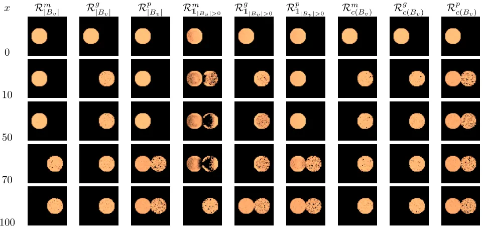
Experiment 3 focuses on the issue of global and local items: Consider, e.g., a budgeting scenario with some city-level projects and some neighborhood-city-level projects. Ide-ally, we would want some mix of city-level projects and neighborhood-level projects to be funded. While it is pos-sible to achieve some mix artificially (e.g., requiring vot-ers to select both city-level projects and neighborhood-level projects), here we are interested in finding out the natural mix that rules in our framework achieve.
Experiment 3 (depicted in Table 4).We have: (1)20 vot-ers, positioned uniformly on the whole1×1square; (2)5 items, termedglobal items, which are also positioned uni-formly on the square; and another 30 items, termed local items, also positioned uniformly on the square; (3) each global item and each local item costs5; (4) we vary the bud-get limit between20and50; (5) the approval sets of the vot-ers are populated with respect to a parameterp, as follows:
For each pair of a voter and a global item, we let the voter approve the global item with some probabilityp. For each pair of a voter and a local item, we let the voter approve the local item if and only if their Euclidean distance is at most 0.2. In Table 4 each datapoint is averaged over100 repeti-tions and we consider the average funds spent on local items as a function of the probabilitypof approving a global item.
Experimental Results
Next we discuss the results of our experiments, depicted in Tables 2, 3, and 4.
In Table 2, and focusing on the Max rules, it is visi-ble that Rm
c(Bv) prefers expensive items the most, R
m
|Bv|
prefers expensive items the least, whileRm
1|Bv|>0 is
some-how in between. This can be seen specifically by notic-ing thatRm
|Bv|ceases to select expensive items as soon as
x = 30, Rm
1|Bv|>0 ceases to select expensive items only
whenx= 190, whileRm
c(Bv)keeps on selecting expensive
items even whenx= 190. Intuitively, this is so as expensive items are useful for Rm
c(Bv) and not useful for R
m
|Bv|; for Rm
1|Bv|>0, while the costs of the items are not useful, their
positions are, as the rule’s goal is to satisfy as many voters as possible. The greedy rules are also somehow in between the extremes, while, as expected, the proportional greedy rules prefer cheaper items.
This general behavior is consistent with Experiment2, as can be seen in Table 3. Specifically, observe that Rm
c(Bv)
switches to funding only expensive items as soon asx= 10, whileRm
|Bv|switches to funding only expensive items only
whenx = 70; due to the positions of the expensive items, and due to the fact that they cover different sets of voters,
Rm
1|Bv|>0 interleave cheap items with expensive items
(ex-cept for the corner cases ofx= 0andx= 100).
As for locality issues, the results depicted in Table 4 for
` = 20 demonstrate that Rm
c(Bv) starts to consider global
items first, withRm
|Bv|after it, andR
m
1|Bv|>0 being the last
to consider global items. As`increases,Rm
c(Bv)andR
m
|Bv|
select more local items whileRm
1|Bv|>0is not affected.
One particularly interesting observation from our experi-ments is that the greedy rule used by Goel (2015),Rg|B
v|in
our language, behaves substantially differently from its Max variant,Rm
|Bv|. This is quite visible in the first two columns
of Tables 2 and 3. The Max variant gives much more atten-tion to the cheap items than the greedy one. Thus the choice between these two rules—already made by many users of Goel’s work—may have nonnegligible consequences.
Outlook
E.g., our results show that, whileRg|B
v|is used extensively
in practice (see, e.g., Goel et al. 2015), it produces signifi-cantly different results than the rule which it approximates, namelyRm
|Bv|.
An immediate future research direction would be to study more satisfaction functions and ways of using them, which would correspond to more rules within our framework. Fur-thermore, defining and studying more axiomatic properties which are relevant to budgeting methods, as well as perform-ing more extensive experimental analysis on various budget-ing methods would help in better understandbudget-ing these rules. Another avenue for future research is to seek general re-sults for rules in the framework, such as identifying classes of rules within the framework which satisfy certain ax-iomatic properties, and better understanding which budget-ing methods reside within the framework and which do not.
Acknowledgments. Piotr Faliszewski was supported by the National Science Centre, Poland, under project 2016/21/B/ST6/01509.
References
Aziz, H.; Faliszewski, P.; Grofman, B.; Slinko, A.; and Tal-mon, N. 2018. Egalitarian committee scoring rules. In Proceedings of the 27th International Joint Conference on Artificial Intelligence (IJCAI ’18), 56–62.
Aziz, H.; Lee, B.; and Talmon, N. 2017. Proportionally rep-resentative participatory budgeting: Axioms and algorithms. arXiv preprint arXiv:1711.08226.
Benade, G.; Nath, S.; Procaccia, A. D.; and Shah, N. 2017. Preference elicitation for participatory budgeting. In Pro-ceedings of the 31st AAAI Conference on Artificial Intelli-gence (AAAI ’17), 376–382.
Cabannes, Y. 2004. Participatory budgeting: a significant contribution to participatory democracy. Environment and urbanization16(1):27–46.
Caragiannis, I.; Nath, S.; Procaccia, A. D.; and Shah, N. 2017. Subset selection via implicit utilitarian voting. Jour-nal of Artificial Intelligence Research58:123–152.
Chamberlin, B., and Courant, P. 1983. Representative de-liberations and representative decisions: Proportional repre-sentation and the Borda rule. American Political Science Review77(3):718–733.
Elkind, E.; Faliszewski, P.; Laslier, J.-F.; Skowron, P.; Slinko, A.; and Talmon, N. 2017a. What do multiwinner voting rules do? An experiment over the two-dimensional Euclidean domain. InProceedings of the 31st AAAI Confer-ence on Artificial IntelligConfer-ence (AAAI ’17), 494–501. Elkind, E.; Faliszewski, P.; Skowron, P.; and Slinko, A. 2017b. Properties of multiwinner voting rules. Social Choice and Welfare48(3):599–632.
Fain, B.; Munagala, K.; and Shah, N. 2018. Fair allocation of indivisible public goods. InProceedings of the 2018 ACM Conference on Economics and Computation (EC’ 18), 575– 592.
Faliszewski, P., and Talmon, N. 2018. Between propor-tionality and diversity: Balancing district sizes under the
Chamberlin-Courant rule. InProceedings of the 17th Inter-national Conference on Autonomous Agents and MultiAgent Systems, 14–22.
Faliszewski, P.; Skowron, P.; Slinko, A.; and Talmon, N. 2016a. Committee scoring rules: Axiomatic classification and hierarchy. InProceedings of the 27nd Joint Conference on Artifical Intelligence (IJCAI ’16), 250–256.
Faliszewski, P.; Skowron, P.; Slinko, A. M.; and Talmon, N. 2016b. Multiwinner analogues of the Plurality rule: Ax-iomatic and algorithmic perspectives. InProceedings of the 30th AAAI Conference on Artificial Intelligence (AAAI ’16), 482–488.
Faliszewski, P.; Szufa, S.; and Talmon, N. 2018. Optimization-based voting rule design: The closer to Utopia the better. InProceedings of the 17th International Confer-ence on Autonomous Agents and MultiAgent Systems, 32– 40.
Feige, U. 1998. A threshold of lnn for approximating set cover.Journal of the ACM45(4):634–652.
Fluschnik, T.; Skowron, P.; Triphaus, M.; and Wilker, K. 2017. Fair Knapsack. arXiv preprint arXiv:1711.04520. Garey, M. R., and Johnson, D. S. 1979. Computers and intractability: A guide to the theory of NP-completeness. Gilman, H. R. 2012. Transformative deliberations: Partici-patory budgeting in the united states. Journal of Public De-liberation8(11).
Goel, A.; Krishnaswamy, A. K.; Sakshuwong, S.; and Aita-murto, T. 2015. Knapsack voting.Collective Intelligence. Goel, A.; Krishnaswamy, A. K.; and Sakshuwong, S. 2016. Budget aggregation via Knapsack voting: welfare-maximization and strategy-proofness. Collective Intelli-gence783–809.
Gurobi Optimization, L. 2018. Gurobi optimizer reference manual.
Lackner, M., and Skowron, P. 2017. Consistent approval-based multi-winner rules.arXiv preprint arXiv:1704.02453. Laslier, J.-F., and Sanver, R., eds. 2010. Handbook on Ap-proval Voting. Springer.
Lu, T., and Boutilier, C. 2011. Budgeted social choice: From consensus to personalized decision making. InProceedings of the 20th International Joint Conference on Artificial In-telligence (IJCAI ’11), volume 11, 280–286.
Procaccia, A. D.; Rosenschein, J. S.; and Zohar, A. 2008. On the complexity of achieving proportional representation. Social Choice and Welfare30(3):353–362.
Shapiro, E., and Talmon, N. 2017. A Condorcet-consistent participatory budgeting algorithm.arXiv preprint arXiv:1709.05839.
Skowron, P., and Faliszewski, P. 2017. Chamberlin-Courant rule with approval ballots: Approximating the MaxCover problem with bounded frequencies in FPT time. Journal of Artificial Intelligence Research60:687–716.