R E S E A R C H
Open Access
Notes on interval halving procedure for
periodic and two-point problems
András Rontó
1*, Miklós Rontó
2and Nataliya Shchobak
3,4*Correspondence:
1Institute of Mathematics, Academy
of Sciences of Czech Republic, 22 Žižkova St., Brno, 616 62, Czech Republic
Full list of author information is available at the end of the article
Abstract
We continue our study of constructive numerical-analytic schemes of investigation of boundary problems. We simplify and improve the recently suggested interval halving technique allowing one to essentially weaken the convergence conditions.
MSC: Primary 34B15
Keywords: periodic solution; two-point problem; Lyapunov-Schmidt reduction; determining equation; parametrisation; periodic successive approximations; numerical-analytic method; Cesari method; interval halving
1 Introduction
The present note is a continuation of [] and deals with a constructive approach to the investigation of two-point boundary value problems. The approach is numerical-analytic [, ] in the sense that, although part of the computation is carried out analytically, the fi-nal stage of the method involves a numerical afi-nalysis of certain equations usually referred to asdetermining, orbifurcation, equations. This scheme of Lyapunov-Schmidt type [, ] reminds one of the shooting method on first glance, but there are several essential differ-ences [].
We consider the periodic boundary value problem
u(t) =ft,u(t), t∈[,p], ()
u() =u(p), ()
wherep∈(,∞),f : [,p]×Rn→Rnsatisfies the Carathéodory conditions, and a
solu-tion is an absolutely continuous vector funcsolu-tion satisfying () almost everywhere on [,p]. Our main assumption till the end of the paper is that there exist a certain matrixKand a bounded closed set⊂Rnsuch thatf(t,·)∈LipK() for a.e.t∈[,p]. Here and below, given a square matrixKwith non-negative entries,LipK() stands for the set of functions
g:→Rnsatisfying the componentwise Lipschitz condition
g(z) –g(z)≤K|z–z| ()
for allzandzfrom. In () and all similar relations that will appear below, the symbols
≤and| · |are understood componentwise.
In its original form (see,e.g., [, ] for references), the numerical-analytic approach that we are dealing with suggests one to look for a solution of (), () among the limit functions of certainn-parametric family of sequences possessing property () (see,e.g., [, ]). Given an arbitrary vectorξ, consider the sequence of functions defined by the recurrence relation
um(t,ξ) :=ξ+
t
fs,um–(s,ξ)
ds– t
p
p
fs,um–(s,ξ)
ds, t∈[,p], ()
withm= , , . . . andu(t,ξ) :=ξ,t∈[,p]. Clearly, each of functions () satisfies the peri-odic boundary condition (). If one establishes the existence of the limit
u∞(·,ξ) := lim
m→∞um(·,ξ), ξ∈, ()
with a certain⊂D, one finds out that the existence of a solutionu(·) of the periodic problem (), () with the value at zero lying in is equivalent to the solvability of the equation
p
fs,u∞(s,ξ)ds=
with respect to the unknown vectorξ. This leads to a Lyapunov-Schmidt type reduction of the periodic problem (see [, ] for more details), which is known to be applicable on the assumption that
f(t,·)∈LipK(D) for a.e.t∈[,p], ()
withpK small enough andDsatisfying the condition
D
T
δD(f)
=∅, ()
where
δD(f) :=max
δ[,p/],D(f),δ[p/,p],D(f) ()
andδJ,V(f) :=max(t,ξ)∈J×Vf(t,ξ) –min(t,ξ)∈J×Vf(t,ξ) for any compactV⊆DandJ⊆[,p].
In (),D() is the-coreofDdefined as
D() :=z∈D:B(z,)⊂D ()
for any non-negative vector, where
B(z,) :=ξ∈Rn:|z–ξ| ≤ ()
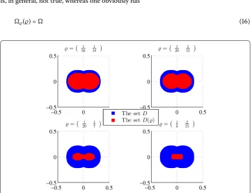
Figure 1 The setD() in examples,= col(1/12, 1/18).
The main limitation of this approach is that, in order to guarantee the convergence, one has to assume a certain smallness of the eigenvalues of the matrixpK. It was shown, in particular, in [] that the method based upon sequence () is applicable provided that
r(K) <
γp
, ()
where
γ:=
. ()
Moreover, as is seen from condition (), the setDwhere () holds should be wide enough (in particular, such thatdiamD≥pδD(f), with the natural componentwise definition of a
vector-valued diameter of a set).
As the recent paper [] shows, the limitation can be overcome by noticing that the quan-tity which is assumed be small enough is always proportional to the length of the interval. A natural interval halving technique then allows one to produce a version of the scheme where () is replaced by the condition
r(K) <
γp
and, thus, weakened by half. A similar improvement is also achieved in relation to condi-tion (), which is replaced by the assumpcondi-tion that
D
T
δD(f)
=∅. ()
Clearly, the transition to () weakens () by half.
restrictive. Indeed, the idea to start from a setDwhere the nonlinearity is known to be Lipschitzian and look for its suitable subsetD() that could potentially contain initial val-ues of periodic solutions is somewhat unnatural because, in any case, it is the initial valval-ues that are of major interest, the regularity assumptions for the equation being only technical assumptions induced by the method. Instead of doing so, which used to be the case in [] and in all the previous works, it is, however, more logical to choose a closed bounded set
⊂Rn, where one expects to find initial values of the solution, and to assume that the
nonlinearity is Lipschitzian on a suitable˜ ⊃, with˜ only as large as the method re-quires. It is not difficult to see that the argument of [] then leads us to the choice˜ :=,
whereis the-neighbourhoodofin the sense that
:=
ξ∈
B(ξ,), ()
where the symbol B(ξ,) stands for the-neighbourhood of a vectorξ (recall that the relations in () are componentwise). Besides its more natural character, the use of the pair of sets (,) is also advantageous in contrast to (D,D()) because, geometrically,D()
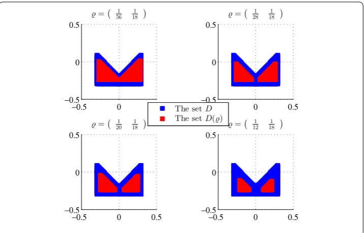
does not necessarily copy the shape ofD(see Figures and for examples whereDand the correspondingD() with=
gradually increasing are represented, respectively, by the blue and red regions). In fact, the operations of taking-core and-neighbourhood do not commute: the equality in the inclusion
D()⊂D ()
is, in general, not true, whereas one obviously has
() = ()
Figure 3 An example ofDwithD() disconnected for certain.
Figure 4 An example of the setDillustrating the strict inclusion in (15).
for any. The strict inclusion in () holds, in particular, in the example from Figure , where the points of the setsD(),Dand (D())for several values of=
,≤, are plotted in red, blue and cyan, respectively. In that example, by choosingto be the red region, one should then widen it for the technical purposes related to the method up to the cyan one, and not the blue one. A comparison of () and () confirms the advantage of assuming conditions of type () on. Several examples of domainsand
the corresponding setscan be seen on Figure .
Using the (,) setting, we further reformulate the scheme of the method further by
Figure 5 The setin examples,= col(1/8, 1/16).
the approach to problems with two-point boundary conditions different from the periodic ones, which technique is also outlined in what follows.
2 Construction of iterations and proof of convergence
Thus, let us fix a closed bounded set⊂Rn, where the initial values of solutions of prob-lem (), () will be looked for. Without loss of generality, we shall chooseto be convex. Letξandηbe arbitrary vectors from. Let us put
x(t,ξ,η) :=
–t
p
ξ+t
pη, t∈[,p/], ()
y(t,ξ,η) :=
– t
p
η+
t p –
ξ, t∈[p/,p], ()
and define the recurrence sequences of functions xm : [,p/]× → Rn and ym :
[p/,p]×→Rn,m= , , . . . , according to the formulae
xm(t,ξ,η) :=x(t,ξ,η) +
t
fs,xm–(s,ξ,η)
ds
–t
p
p
fs,xm–(s,ξ,η)
ds, t∈[,p/], ()
ym(t,ξ,η) :=y(t,ξ,η) +
t
p
fs,ym–(s,ξ,η)
ds
–
t p –
p
p
fs,ym–(s,ξ,η)
ds, t∈[p/,p], ()
where m≥. One arrives at formulae (), () directly when choosing x(·,ξ,η) and
y(·,ξ,η) as linear functions on the appropriate intervals satisfying the equalities
x(,ξ,η) =ξ, x
p
,ξ,η
y
p
,ξ,η
=η, y(p,ξ,η) =ξ. ()
The considerations in [] concerning the auxiliary parametrised problems (.), (.) and (.), (.) can be omitted. Clearly, () and () are the simplest choice of functions sat-isfying () and ().
The form of sequences (), () is motivated by the following proposition.
Proposition Let(ξ,η)∈be fixed.If the limits x∞(·,ξ,η)and y∞(·,ξ,η)of sequences
()and(),respectively,exist uniformly on[,p]and[p,p],then: . The functionx∞(·,ξ,η)has the property
x∞
p
,ξ,η
–x∞(,ξ,η) =η–ξ ()
and is the unique solution of the initial value problem
x(t) =ft,x(t)+
p(ξ,η), t∈[,p/], ()
x() =ξ, ()
where
(ξ,η) :=η–ξ– p
fτ,x∞(τ,ξ,η)dτ. ()
. The functiony∞(·,ξ,η)has the property
y∞(p,ξ,η) –y∞
p
,ξ,η
=ξ–η ()
and is the unique solution of the initial value problem
y(t) =ft,y(t)+
pH(ξ,η), t∈[p/,p], ()
y
p
=η, ()
where
H(ξ,η) :=ξ–η– p
p
fτ,y∞(τ,ξ,η)dτ. ()
The proposition stated above, which is an easy consequence of the definitions of the functionsxm: [,p/]×→Rnandym: [p/,p]×→Rn,m= , , . . . , suggests one
to consider the functionu∞(·,ξ,η) : [,p]→Rnintroduced according to the formula
u∞(t,ξ,η) := ⎧ ⎨ ⎩
x∞(t,ξ,η) ift∈[,p/],
for allξ andηfromand look for solutions of problem (), () in the formu∞(·,ξ,η). Note that, as follows immediately from (), () and (),
x∞
p
,ξ,η
=y∞
p
,ξ,η
and, therefore, the functionu∞(·,ξ,η) is continuous on [,p] for any (ξ,η)∈. The use of this function, however, requires the knowledge of the fact thatx∞(·,ξ,η) andy∞(·,ξ,η) are well defined for (ξ,η)∈.
Introduce the functions
¯
α(t) :=
pt(p–t), t∈[,p/] ()
and
¯¯
α(t) :=
p(p– t)(t– p), t∈[p/,p]. ()
Theorem If there exists a non-negative vectorwith the property
≥p
δ(f) ()
such that f(t,·)∈LipK()for a.e.t∈[,p]with a certain K and
r(K) <
γp
()
then,for all fixed(ξ,η)∈,the sequence{xm(·,ξ,η) :m≥}(resp.,{ym(·,ξ,η) :m≥}) converges to a limit function x∞(·,ξ,η) (resp.,y∞(·,ξ,η))uniformly in t∈[,p/] (resp.,
t∈[p/,p]),and the following estimates hold:
xm(·,ξ,η) –x∞(t,ξ,η)≤α¯(t) m+(γpK)
m
n–
γp K
–
δ[,p/],(f) ()
for all t∈[,p/]and
ym(·,ξ,η) –y∞(t,ξ,η)≤α¯¯(t) m+(γpK)
m
n–
γp K
–
δ[p/,p],(f) ()
for all t∈[p/,p]and m≥.
In estimates () and (), the symbolnstands for the unit matrix of dimensionn. Recall
also thatγ= /, as indicated above. Note that condition () can be slightly improved by replacingγby the constant
γ∗≈. ()
is not actually of primary importance since the very aim of the interval halving technique discussed here is to weaken assumption () by half and, in any case, the difference be-tween the two conditions is quite insignificant becauseγ–γ∗≈..
Remark It follows from [, Lemma .] that estimates () and () can be shown to
hold for allm≥ if the definition of functionsα¯andα¯¯is changed slightly (namely, the multiplier / is added on the right-hand side of (), ()).
It should be mentioned that assumption (), which, by Theorem , ensures the applica-bility of the iteration scheme based on formulae (), (), is twice as weak as assumption () for the original sequence (). The same kind of improvement is achieved concerning the condition on the setDwheref is Lipschitzian since, for the scheme without interval halving, one would require that
∃: ≥p
δ(f), ()
which is twice as strong as (). In contrast to the related assumptions from [] and earlier works, condition () is easier to verify because in order to do so one has only to find the valueδ(f), which is computed directly by estimatingf. In addition, it is possible to
estimate this value in certain cases where some further information on the behaviour off
is known.
Comparing Theorem with Theorems . and . of [], where the values in (.) and (.) are computed over the entire domain wheref is Lipschitzian, we see that the values
δ[,p/],(f) andδ[p/,p],(f) in Theorem are computed overonly.
The proof of Theorem is carried out by a suitable modification of that of [, Theo-rem .] and is based upon the following lemmata.
Lemma ([, Lemma .]) Let x: [,p/]→Rnand y: [p/,p]→Rnbe arbitrary func-tions such that{x(t) :t∈[,p/]} ⊂and{y(t) :t∈[p/,p]} ⊂.Then
Pf
·,x(·)(t)≤
α¯(t)δ[,p/],(f)
≤p
δ[,p/],(f) ()
for t∈[,p/]and
Pf
·,y(·)(t)≤
α¯¯(t)δ[p/,p],(f)
≤p
δ[p/,p],(f) ()
for t∈[p/,p].
In (), (), the mappingsPandPare defined by the equality
(Piv)(t) :=
t
i
p
v(s)ds–
t p –i
i+ p
i
p
v(s)ds ()
Lemma Letbe a vector satisfying relation().Then,for arbitrary m≥and(ξ,η)∈
,the inclusions
xm(t,ξ,η) :t∈[,p/] ⊂ ()
and
ym(t,ξ,η) :t∈[p/,p] ⊂ ()
hold.
Proof Letξ andηbe arbitrary vectors from. It is natural to argue by induction. Since
is assumed to be convex, it follows from () thatx(t,ξ,η)∈for anyt∈[,p/] and
y(t,ξ,η)∈for anyt∈[p/,p],i.e., () and () are true form= . Let us assume that () and () hold for a certainm=m.
Considering relations (), (), (), () and () and using Lemma , we obtain
xm+(t,ξ,η) –x(t,ξ,η)=Pf
·,xm(·,ξ,η)(t)
≤p
δ[,p/],(f)
≤ ()
fort∈[,p/] and
ym
+(t,ξ,η) –y(t,ξ,η)=Pf
·,ym(·,ξ,η)(t)
≤p
δ[p/,p],(f)
≤ ()
fort∈[p/,p]. Since () and () are satisfied form= , we see from (), () that all the values ofxm+(·,ξ,η) andym+(·,ξ,η) are contained in a-neighbourhood of a point
from, which means that () and () hold form=m+ . It now remains to use the
arbitrariness ofm.
The assertion of Theorem is now obtained by replacing [, Lemma .] by Lemma and arguing by analogy to the proof of Theorems . and . from []. Furthermore, sim-ilarly to [], using Proposition and Theorem , one arrives at the following.
Theorem Assume that f(t,·)∈LipK()for a.e.t∈[,p],whereis a vector with prop-erty()and K satisfies condition().Then,for every solution u(·)of problem(), ()with the property
u(t)|t∈[,p] ⊂ and
u(),u
p
⊂, ()
(ξ,η)satisfies the system ofn equations
(ξ,η) = , H(ξ,η) = .
()
Recall that the functions:→Rnand H :→Rnare defined according to
equal-ities () and (), and the latter equalequal-ities make sense in view of Theorem .
3 Constructive solvability analysis
Theorem provides one a formal reduction of the periodic problem (), () to the system of nnumerical equations () in the sense that the initial data (u(),u(p/)) of any so-lution of (), () with properties () can be found from (). Thus, under the conditions assumed, the question on solutions of the periodic boundary value problem (), () can be replaced that of the system of numerical equations (). A combination of Proposition and Theorems , then suggests one a scheme of investigation of the periodic boundary value problem (), (). The practical realisation of the scheme is based upon the so-called approximate determining functions
m(ξ,η) :=η–ξ–
p
fτ,xm(τ,ξ,η)
dτ, ()
Hm(ξ,η) :=ξ–η–
p
p
fτ,ym(τ,ξ,η)
dτ, ()
considered for a fixed value of mand, thus, computable explicitly. Then, as in [], the function
um(t,ξ,η) :=
⎧ ⎨ ⎩
xm(t,ξ,η) ift∈[,p/], ym(t,ξ,η) ift∈(p/,p],
()
can be used to obtain themth approximation to a solution of problem (), () provided that we are able to find certainξ andηsatisfying themth approximate determining equations
m(ξ,η) = ,
Hm(ξ,η) = .
()
Furthermore, it turns out that, under natural conditions, the solvability of the periodic problem (), () can be derived from that of system (). More precisely, putting
m(ξ,η) :=
η–ξ–pf(p–τ,xm(p–τ,ξ,η))dτ
ξ–η–pf(p+τ,ym(p+τ,ξ,η))dτ
()
and
∞(ξ,η) :=
η–ξ–
p
f(
p–τ
,x∞(
p–τ
,ξ,η))dτ
ξ–η–pf(p+τ,y∞(p+τ,ξ,η))dτ
()
Theorem Let f(t,·)∈LipK()for a.e.t∈[,p],whereis a vector with property() and K satisfies condition().Moreover,assume thatmsatisfies the condition
deg(m,)= ()
for a certain fixed m≥and there exists a continuous mapping Q: [, ]×which does not vanish on(, )×∂ and is such that Q(,·) =m,Q(,·) =∞.Then there exists
a pair(ξ∗,η∗)∈ such that the function u:=u
∞(·,ξ∗,η∗)is a solution of the periodic
boundary value problem(), ()possessing properties().
It should be noted that the vector fieldm is finite-dimensional and, thus, the degree
involved in () is the Brower degree.
Proof We can rely on the argument from the proof of [, Theorem .]. Indeed, a certain computation based on () shows that
m(ξ,η) =
m(ξ,η)
Hm(ξ,η)
()
for all (ξ,η)∈and, thus, () is necessary and sufficient for (ξ,η) to be a singular point ofm. Similarly to [], the assumptions of the theorem then allow one to construct a
non-degenerate deformation ofminto the vector field
(ξ,η)→
(ξ,η) H(ξ,η)
the singular points of which determine solutions of problem (), () satisfying condition (), and use the homotopy invariance of the degree. The remaining property in () is a
consequence of Lemma .
Let the binary relationSbe defined [] for anyS⊂Rnas follows: functionsg= (gi)i=n : Rn→Rnandh= (h
i)i=n :Rn→Rnare said to satisfy the relationgShif and only if
there exists a functionν:S→ {, , . . . , n}such thatgν(z)(z) >hν(z)(z) at every pointz∈S. Using this relation, one can formulate an efficient condition sufficient for the solvability of problem (), ().
Corollary Let f(t,·)∈LipK()for a.e.t∈[,p],wheresatisfies inequality()and K has property().Let,moreover,
|m|∂
p
Mmδ[,p/],(f) Mmδ[p/,p],(f)
()
for a certain fixed m≥,where
Mm:=
γp
m+
Km+
n–
γp K
–
. ()
Then there exists a pair(ξ∗,η∗)∈such that u:=u
Proof It is sufficient to apply Theorem with the linear homotopy
Q(θ,ξ,η) := ( –θ)m(ξ,η) +θ ∞(ξ,η) ()
for (ξ,η)∈,θ∈[, ], and use estimate (.) from []. Recall thatγin () is given by (). It is important to emphasise that conditions of Corollary are assumed for afixed m, and all the values depending on it are evaluated in finitely many steps.
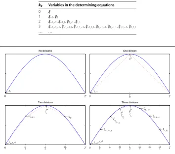
The next assertion is interesting especially because it is, in fact, based upon properties of the starting approximation and, thus, shows how a useful information can be obtained when no iterations have been carried out at all. Note that the zeroth approximation is very rough indeed in any case: the periodic solution is approximated by a piecewise linear function (see Figure ).
With the given functionf involved in (), we associate the functionf#:→Rnby
putting
f#(ξ,η) :=
η–ξ–
p
f(
p–τ
,
τ pξ+ ( –
τ p)η)dτ
ξ–η–pf(p+τ,τpξ+ ( –τp)η)dτ
()
for any (ξ,η)∈. Note that, unlikef, the functionf# depends on the phase variables
only.
Corollary Assume that there is awith property()and f(t,·)∈LipK(),t∈[,p], with K satisfying inequality().Let,furthermore,
degf#,= ()
and
f#∂
p
K(n–γpK)–δ[,p],D(f) K(n–γpK)–δ[p,p],D(f)
. ()
Then the p-periodic problem(), ()has at least one solution u(·)which possesses proper-ties().
Proof Equalities (), (), () and () imply thatf#=. It is also easy to verify by computation that condition () can be rewritten in the form
||∂
p
˜
Mδ[,p/],(f) ˜
Mδ[p/,p],(f)
, ()
4 Discussion
Theorems of the kind specified above allow one to study the periodic problem (), () fol-lowing the lines of [, ]. This analysis is constructive in the sense that the assumptions can be verified efficiently and the results of computation, regarded at first only as candidates for approximate solutions, simultaneously open a way to prove the solvability in a rigorous manner. As regards the computation of iterations themselves, it is helpful to apply suit-able simplified versions of the algorithm, not discussed here, which are better adopted for use with computer algebra systems. The use of polynomial approximations under similar circumstances was considered, in particular, in [].
It is interesting to note thatf#involved in Corollary can be considered as a ‘halved’
analogue of the averaged map
¯ f(ξ) :=
p
f(s,ξ)ds ()
forx∈, which arises similarly tof#in the situation where no interval halving is carried
out. In the latter case, one has the following statement, which is a reformulation of [, Corollary .].
Corollary Let there exist somewith property().Let
deg(f¯,)= ()
and f(t,·)∈LipK(),t∈[,p],with K satisfying inequality().If
|¯f|∂
p
K(n–γpK) –δ
(f), ()
then the p-periodic problem(), ()has a solution u(·)with properties().
Assumption () withf¯given by () arises frequently in topological continuation the-orems where the homotopy to the averaged equation is considered (see,e.g., [, ]).
It should also be noted that, as a natural extension of the above said, one can consider a scheme with multiple interval divisions. Although the addition of intermediate nodes increases the number of equations to be solved numerically (atkinterval halvings, one ultimately arrives a system of kdetermining equation with respect to kvariables), the
important gain is the ability to apply the method regardless of the value of the Lipschitz constant.
The construction of such a scheme is based on the appropriate modification of the initial approximation, which will then depend on more parameters. Consider,e.g., the transition fromk= tok= . Renaming the variables asξ= (ξ–,ξ) in the former case for more convenience and denoting the initial approximation byu(·,ξ), we rewrite (), () in the form
u(,ξ) =ξ–, u
p
,ξ
=ξ, u(p,ξ) =ξ–. ()
tree graph like notation to the case of two interval halvings (k= ) and arguing similarly, we arrive at the following equalities determiningu(·,ξ):
u(,ξ) =ξ–,–, u
p
,ξ
=ξ–,, u
p
,ξ
=ξ,–,
u
p
,ξ
=ξ,, u(p,ξ) =ξ–,–.
()
In other words, relations () mean that the functionu(·,ξ) fork= depends on the array of parametersξ = (ξ–,–,ξ–,,ξ,–,ξ,) and is obtained by the linear interpolation of the points (,ξ–,–), (p,ξ–,), (p,ξ,–), (p,ξ,–), (p,ξ,) and (p,ξ–,–). Fork≥, the structure ofu(·,ξ) is completely analogous, the idea is clear from Table and Figure : one simply draws a broken line joining the corresponding nodes. Onceu(·,ξ) is constructed, the formulae for the subsequent approximations are derived automatically by rescaling the projection map to the corresponding subintervals (we do not need the corresponding explicit formulae here and, therefore, omit the details).
This observation leads one to the following algorithm of investigation of the periodic problem (), ():
Table 1 Variables involved in the determining equations for the respective number of interval halvings
k0 Variables in the determining equations
0 ξ
1 ξ–1,ξ1
2 ξ–1,–1,ξ–1,1,ξ1,–1,ξ1,1
3 ξ–1,–1,–1,ξ–1,–1,1,ξ–1,1,–1,ξ–1,1,1,ξ1,–1,–1,ξ1,–1,1,ξ1,1,–1,ξ1,1,1
. . . .
. Fix a certainkand consider the scheme withkinterval divisions. Fix anmand constructum(·,ξ)form= , , . . . ,m.
. Solve themth approximate determining equations forξ, find a rootξ[m], and put
Um(t) :=um
t,ξ[m], t∈[,p],m= , , . . . ,m. () In the case the equation has multiple roots,()and the related analysis are repeated for each of them (one can study multiple solutions of the original problem in this way).
. ‘Check’ the behaviour of the functionsU,U, . . . ,Um(the heuristic step). If
promising (i.e., there are some signs of convergence), choose a suitable
containing the graph ofUm, find afrom the condition
≥ p
k+δ(f), ()
compute the Lipschitz matrixKforf in, and verify the convergence condition
r(K) <
k
γp
. ()
If not successful with either()or(), increasekappropriately and try again. . Verify conditions of the existence theorem forandm. If not satisfied, or if the
precision ofUmis insufficient, pass tom=m+ and studyUm+. Otherwise the
algorithm stops, and the outcome is:
(a) there is a solutionuof(),()andu≈Um;
(b) ∃(ξ∗,η∗)∈:u(·) =u∞(·,ξ∗,η∗);
(c) the space localisation of the graph ofuis described by properties().
Note the role of interval divisions in the algorithm: forKnot satisfying the smallness condition () andk= (i.e., whenumis constructed according to () without any interval
divisions), the algorithm would stop at step without any result. However, it is obvious that () and () are both satisfied ifkis chosen to be large enough.
In relation to the last remark, it is interesting to compare the approach discussed here with the Cesari method [], which likewise provides one a way to reduce the periodic problem (), () to a system of finitely many numerical equations. The idea of construction of the iterations there is based, in the notation of [], on the use of the operator
Hmu:=L–PmL ()
in a suitable space ofp-periodic functions, where
(Ly)(t) := t
y(s)ds– t
p
p
y(s)ds, t∈[,p],
mis fixed, andPmstands for themth partial sum of the Fourier series of the corresponding
depends on the Lipschitz constant off as well (in fact, it grows withm, the convergence being guaranteed by suitable properties ofHm formlarge enough), which reminds us of
Table in our case. The approach presented in this note, in our opinion, has the advan-tage that, firstly, the computation of iterations is significantly simpler (apart of the integral mean, one does not need to compute any higher order terms in the Fourier expansion) and, secondly, it can be used for other problems as well, whereas, due to the nature of formula (), the use of Cesari’s scheme is limited to periodic functions.
In particular, the method described above is rather easy to adopt for application to two-point boundary value problems different from the periodic ones. Indeed, consider the problem with linear two-point conditions where one of the coefficient matrices is non-singular. Without loss of generality, we can assume that the problem has the form
u(t) =ft,u(t), t∈[,p], ()
u(p) –Au() =c, ()
whereAis a square matrix of dimensionn(possibly, singular),c∈Rn,f : [,p]×Rn→Rn,
andp∈(,∞).
The transition from the periodic problem (), () to problem (), () is then surpris-ingly simple: one does not need but to adjust the functionsx(·,ξ,η) andy(·,ξ,η) so that they satisfy the boundary condition (). More precisely, let us fix a suitableand take arbitraryξ andηin it. Introduce the sequences of functionsxm: [,p/]×→Rnand ym: [p/,p]×→Rn,m= , , . . . , according to the same recurrence formulae as in
(), (), where, instead of (), (), the functionsx(·,ξ,η) andy(·,ξ,η) are given by the equalities
x(t,ξ,η) :=
–t
p
ξ+t
pη, t∈[,p/], ()
y(t,ξ,η) :=
– t
p
η+
t p –
(Aξ+c), t∈[p/,p]. ()
Clearly,x(·,ξ,η) andy(·,ξ,η) given by (), () are the linear functions satisfying the equalities
x(,ξ,η) =ξ, x
p
,ξ,η
=η, ()
y
p
,ξ,η
=η, y(p,ξ,η) =Aξ+c, ()
which reduce to (), () ifAis the unit matrix andc= . Then, similarly to Proposition , it is not difficult to prove the following.
Proposition Let(ξ,η)∈be fixed.If the limits x
∞(·,ξ,η)and y∞(t,ξ,η)of sequences ()and()exist,then:
. The functionx∞(·,ξ,η)has the property
x∞
p
,ξ,η
–Ax∞(,ξ,η) =η–Aξ ()
. The functiony∞(·,ξ,η)has the property
y∞(p,ξ,η) –Ay∞
p
,ξ,η
=A(ξ–η) +c ()
and is the unique solution of the initial value problem(),()withHgiven by().
We see from Proposition that properties of sequencesxm(·,ξ,η),ym(·,ξ,η),m≥,
constructed for problem (), () are rather similar to those for the periodic problem (), () (in particular, the definition of functionsand H is the same as in Proposition ). In both cases, the iteration is carried out according to formulae (), (), the only difference being in equalities (), () forx(·,ξ,η) and y(·,ξ,η). As a result, the corresponding limit functions satisfy the boundary conditions (), ().
Based on Proposition , one can develop essentially the same techniques that have been indicated above for the periodic problem (), (). The main difference in the proofs is that, in addition to guaranteeing that the appropriate valuesξshould belong to, we also have to ensure thatAξ+c∈as well. The convergence of iterations is then guaranteed for all
ηfrom the setandξbelonging to its subsetSA,c() defined by the relation
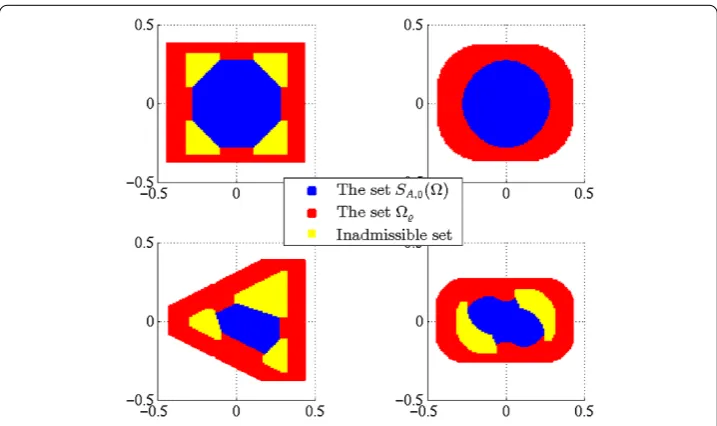
SA,c() :={ξ∈:Aξ+c∈}. ()
Clearly,SA,c() is the union of all the subsets ofinvariant with respect to the
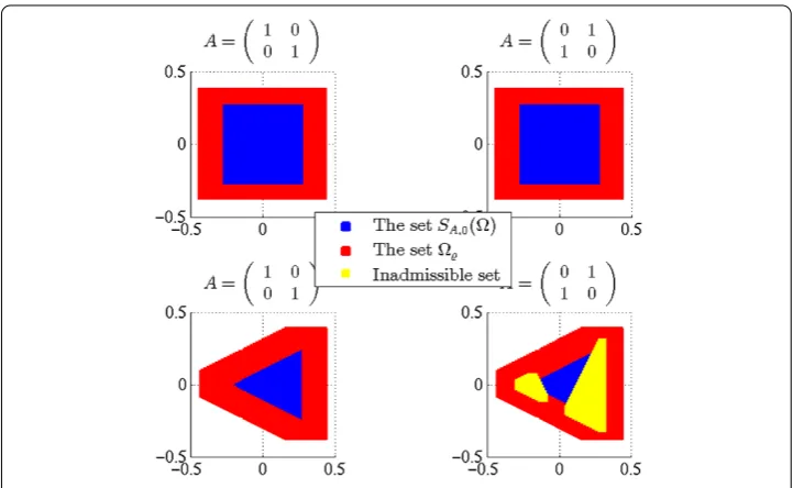
transfor-mationx→Ax+c. For example, ifis a set on the plane (n= ) containing the origin, thenS
( ),
() is the part of that is symmetric with respect to the diagonal passing through the first and the third quadrants (see Figure ).
Theorem Let there exist a non-negative vectorwith property()such that f(t,·)∈
LipK()for a.e.t∈[,p]with a certain matrix K satisfying inequality().Then,for
all fixed (ξ,η)∈SA,c()×,the sequences{xm(·,ξ,η) :m≥}and{ym(·,ξ,η) :m≥} with x(·,ξ,η),y(·,ξ,η)defined by()and()converge uniformly on the corresponding intervals and,moreover,estimates(), ()hold.
The same remark as has been made above concerning Theorem applies to Theorem : its assertion remains true if () is replaced by the inequality
r(K) <
γ∗p
withγ∗given by ().
Theorem is easily obtained by analogy to Theorem for the periodic problem. The verification of the conditions of Theorem is also pretty much similar to the latter case. One has to keep in mind that the techniques for the two-point problem (), () are applicable for the values of parameters lying in SA,c()×, and not in the entire,
which is the case in Theorem (unlessAis the unit matrix andc= ). This circumstance has a natural explanation due to () and (), whence one deduces that bothξandAξ+c
will eventually belong to one and the same set, which fact is then used in Lemma . If, for example,cis equal to zero and
A=√
–
, ()
then the assertion of Theorem is true only for the part ofthat is invariant under the rotation by ◦counter-clockwise. In this way,e.g., Figure is replaced by Figure once the two-point problem (), () withAgiven by () is considered. Note that all the sets on Figures and contain the origin, and the yellow regions on the latter one indicate the points fromthat cannot be regarded as candidates for initial values of the solution in question.
Competing interests
The authors declare that they have no competing interests.
Authors’ contributions
All the authors contributed equally to the final version of this work and approved its present form.
Author details
1Institute of Mathematics, Academy of Sciences of Czech Republic, 22 Žižkova St., Brno, 616 62, Czech Republic. 2Department of Analysis, University of Miskolc, Miskolc-Egyetemváros, Miskolc, 3515, Hungary.3Department of
Mathematics, Uzhgorod National University, 46 Pidhirna St., Uzhgorod, 88 000, Ukraine.4Mathematical Institute, Slovak Academy of Sciences, 49 Štefánikova St., Bratislava, 814 73, Slovakia.
Acknowledgements
The work was supported in part by RVO: 67985840 (A Rontó) and the SAIA National Scholarship Programme of the Slovak Republic (N Shchobak).
Received: 18 March 2014 Accepted: 20 June 2014 References
1. Rontó, A, Rontó, M, Shchobak, N: Constructive analysis of periodic solutions with interval halving. Bound. Value Probl.
2013, 57 (2013). doi:10.1186/1687-2770-2013-57
2. Samoilenko, AM, Rontó, NI: Numerical-Analytic Methods in the Theory of Boundary-Value Problems for Ordinary Differential Equations. Naukova Dumka, Kiev (1992) (in Russian). Edited and with a preface by YA Mitropolskii 3. Rontó, A, Rontó, M: Successive approximation techniques in non-linear boundary value problems for ordinary
differential equations. In: Handbook of Differential Equations: Ordinary Differential Equations, vol. IV, pp. 441-592. Elsevier, Amsterdam (2008)
4. Nirenberg, L: Topics in Nonlinear Functional Analysis. Courant Lecture Notes Series. Am. Math. Soc., New York (1974). With a chapter by E Zehnder, notes by RA Artino, lecture notes, 1973-1974
5. Gaines, RE, Mawhin, JL: Coincidence Degree and Nonlinear Differential Equations. Lecture Notes in Mathematics, vol. 568. Springer, Berlin (1977)
6. Rontó, M, Samoilenko, AM: Numerical-Analytic Methods in the Theory of Boundary-Value Problems. World Scientific, River Edge (2000). doi:10.1142/9789812813602. With a preface by YA Mitropolsky and an appendix by the authors and SI Trofimchuk
7. Rontó, A, Rontó, M, Holubová, G, Neˇcesal, P: Numerical-analytic technique for investigation of solutions of some nonlinear equations with Dirichlet conditions. Bound. Value Probl.2011, 58 (2011). doi:10.1186/1687-2770-2011-58 8. Mawhin, J: Topological Degree Methods in Nonlinear Boundary Value Problems. CBMS Regional Conference Series in
Mathematics, vol. 40. Am. Math. Soc., Providence (1979). Expository lectures from the CBMS Regional Conference held at Harvey Mudd College, Claremont, Calif., June 9-15, 1977
9. Capietto, A, Mawhin, J, Zanolin, F: A continuation approach to superlinear periodic boundary value problems. J. Differ. Equ.88(2), 347-395 (1990). doi:10.1016/0022-0396(90)90102-U
10. Cesari, L: Asymptotic Behavior and Stability Problems in Ordinary Differential Equations, 3rd edn. Ergebnisse der Mathematik und Ihrer Grenzgebiete, vol. 16. Springer, New York (1971)
11. Knobloch, H-W: Remarks on a paper of L. Cesari on functional analysis and nonlinear differential equations. Mich. Math. J.10, 417-430 (1963)
doi:10.1186/s13661-014-0164-9