ABSTRACT
SCHOLCOVER, FEDERICO. Using a Finite Mixture Model-Based Clustering Approach to Identify Move and Wait Strategies (Under the direction of Douglas J. Gillan).
Telerobotic platforms can be sent to places human cannot or should not go. They can
explore space or search a collapsed building for survivors while keeping the human operator
safe. However, distance between the human operator and the platform induces latency – a gap in
time between when the operator sends a command, the platform executes the command, and when the operator receives feedback about the command’s execution. This latency negatively
impacts task performance, and operators assume different strategies to compensate for increased latency. The strategy is known as the “Move and Wait” strategy, where operators make
increasingly piecemeal movements as latency increases. The operators will move a little, wait to
see the results, and then move again. Detection of strategy use has relied on coarse measures:
visual inspection or trial-level outcomes, such as the proportion of time spent waiting. These
measures do not allow for the detection of strategy use in-the-moment. We cannot say that a
participant spent the first part of a trial using a strategy before transitioning to a different
strategy. There is additional anecdotal evidence to suggest the existence of an intermediary
strategy which current measures would be unable to detect. The work here addresses these issues
by developing a novel method to define strategy use, by adapting the PRONET technique to
continuous data. Continuous movement data was transformed into discrete clusters, using finite
mixture models, and the transitions between these clusters were passed to a Pathfinder algorithm.
Results demonstrate (1) this methods utility and (2) at supports the existence of the three
Using a Finite Mixture Model-Based Clustering Approach to Identify Move and Wait Strategies
by
Federico Scholcover
A dissertation submitted to the Graduate Faculty of North Carolina State University
in partial fulfillment of the requirements for the degree of
Doctor of Philosophy
Psychology
Raleigh, North Carolina 2020
APPROVED BY:
_______________________________ _______________________________
Dr. Douglas Gillan Dr. Jing Feng
Committee Chair
_______________________________ _______________________________
DEDICATION
To the countless friends I have made throughout my life, in Florida and in North Carolina. I hope
BIOGRAPHY
Federico “Freddy” Scholcover was born in Buenos Aires, Argentina and immigrated to the
United States at the age of 4. Freddy grew up in Coral Springs, Florida where he developed a
passion for wearing flipflops (as all Floridians should). Freddy earned a pair of B.S. degrees
(with honors) from the University of Central Florida in 2014 before joining NC State’s Human
Factors & Applied Cognition doctoral program. Freddy spent his time at NC State doing a little
bit of everything: researching, teaching, working in industry, mentoring, networking. Now, he
can include “graduating during a global pandemic” to that list. Freddy has accepted a position as
a Postdoctoral Research Scholar with Arizona State University’s Center for Human, Artificial
ACKNOWLEDGEMENTS
First, I would like to thank my advisor Dr. Doug Gillan for one million different reasons: His
expertise, his generosity with his time, his patience with me as I figured out what I wanted to do
when I graduated, for being the example of the researcher, instructor, and mentor that I hope to
be one day (that’s six of the one million reasons). Sincerely, Doug, thank you.
I would also like to thank my committee – Dr. Anne McLaughlin, Dr. Caroline Proulx, Dr. Chris
Mayhorn, and Dr. Jing Feng – for their advice and feedback on this project, as well as all the
other advice and feedback they have given me through the years.
I would also like to acknowledge my parents: Claudio Scholcover, Dave Gonzalez, Maria
Fernanda Golod-Gonzalez. Thank you for being so patient with me.
TABLE OF CONTENTS
LIST OF TABLES ... vii
LIST OF FIGURES ... ix
INTRODUCTION... 1
The Move and Wait Strategy ... 2
PRONET Application of the Pathfinder Network Algorithm ... 4
Clustering as a Means of Data Recovery ... 6
Gaussian Mixture Models ... 8
Current Study ... 11
METHOD ... 12
Magnitude Estimation Task ... 13
Route Navigation Task ... 13
RESULTS ... 16
Model Generation ... 16
Model Selection ... 17
Evaluating Cluster Solutions ... 26
Understanding Movement Patterns with the PRONET Technique ... 28
Predicting Task Outcomes ... 32
DISCUSSION ... 36
Limitations and Future Directions ... 38
Applications 40 Conclusion 41 REFERENCES ... 42
APPENDICES ... 50
Appendix 1. Data Output for each Variable Set ... 51
Appendix 1.1. Move-Only Results ... 51
Appendix 1.2. Move & NASA-TLX Results... 60
Appendix 1.3. Move, NASA-TLX, & Temporal Sensitivity Results ... 69
Appendix 1.4. Move & Temporal Sensitivity Results ... 84
Appendix 1.5. Move & Wait Results ... 93
Appendix 1.6. Move, Wait, & NASA-TLX Results ... 102
Appendix 1.7. Move, Wait, NASA-TLX, & Temporal Sensitivity Results ... 117
Appendix 1.8. Move, Wait, & Temporal Sensitivity Results ... 141
Appendix 1.9. Wait-Only Results ... 156
Appendix 1.10. Wait & NASA-TLX Results ... 165
Appendix 1.11. Wait, NASA-TLX, & Temporal Sensitivity Results ... 174
Appendix 1.12. Wait & Temporal Sensitivity Results ... 189
Appendix 2. R Scripts ... 198
Appendix 2.1 – Data Cleaning ... 198
Appendix 2.2 – Cluster Generation ... 205
Appendix 2.3 – Cluster Combiner (Baudry, et al. 2010 Procedure) ... 210
Appendix 2.4 – Cluster File Reorganizer ... 213
Appendix 2.5 – Cluster Summary Plots and Piecewise Regression ... 216
Appendix 2.6 – Pairwise Adjusted Rand Index ... 229
Appendix 2.8 – Apply Clusters to Test Data ... 237
Appendix 2.9 – Calculate Trial Summaries ... 245
Appendix 2.10 – Inferential Statistics and Plots ... 250
Appendix 2.11 – PRONET Analysis, Appendix Generator and Miscellanea ... 268
LIST OF TABLES
Table 1. Movement Variable Sets to be Used in Clustering. ... 16
Table 2. Trial-Level Variable Sets to be Used in Clustering. ... 16
Table 3. Appendix and Page Number for Variable Set Analysis. ... 18
Table 4. Summary of all 600 runs. ... 19
Table 5. Summary of final candidate models. ... 24
Table 6. Cluster Summary for Move-Only Solution. ... 24
Table 7. Cluster Summary for Wait-Only Solution. ... 26
Table 8. Mean Freq. of Cluster for Move-Only Cluster Solution ... 27
Table 9. Mean Freq. of Cluster for Wait-Only Cluster Solution... 27
Table 10. Linear Mixed-Effects Models for Move-Only Cluster Solution ... 34
Table 11. Mixture Model for Move-Only Solution... 51
Table 12. Cluster Summary for Move-Only Solution. ... 53
Table 13. Mean Freq. of Cluster for Move-Only Solution... 55
Table 14. Count of Cluster Transitions in Test Set for Move-Only Solution. ... 57
Table 15. Linear Mixed-Effects Models for Move-Only Solution. ... 59
Table 16. Mixture Model for Move & NASA-TLX Solution. ... 60
Table 17. Cluster Summary for Move & NASA-TLX Solution. ... 62
Table 18. Mean Freq. of Cluster for Move & NASA-TLX Solution. ... 64
Table 19. Count of Cluster Transitions in Test Set for Move & NASA-TLX Solution. ... 66
Table 20. Linear Mixed-Effects Models for Move & NASA-TLX Solution... 68
Table 21. Mixture Model for Move, NASA-TLX, & Temporal Sensitivity Solution. ... 69
Table 22. Cluster Summary for Move, NASA-TLX, & Temporal Sensitivity Solution. ... 73
Table 23. Mean Freq. of Cluster for Move, NASA-TLX, & Temporal Sensitivity Solution. ... 77
Table 24. Count of Cluster Transitions in Test Set for Move, NASA-TLX, & Temporal Sensitivity Solution. ... 81
Table 25. Linear Mixed-Effects Models for Move, NASA-TLX, & Temporal Sensitivity Solution. ... 83
Table 26. Mixture Model for Move & Temporal Sensitivity Solution. ... 84
Table 27. Cluster Summary for Move & Temporal Sensitivity Solution. ... 86
Table 28. Mean Freq. of Cluster for Move & Temporal Sensitivity Solution. ... 88
Table 29. Count of Cluster Transitions in Test Set for Move & Temporal Sensitivity Solution. ... 90
Table 30. Linear Mixed-Effects Models for Move & Temporal Sensitivity Solution. ... 92
Table 31. Mixture Model for Move & Wait Solution. ... 93
Table 32. Cluster Summary for Move & Wait Solution. ... 95
Table 33. Mean Freq. of Cluster for Move & Wait Solution. ... 97
Table 34. Count of Cluster Transitions in Test Set for Move & Wait Solution... 99
Table 35. Linear Mixed-Effects Models for Move & Wait Solution. ... 101
Table 36. Mixture Model for Move, Wait, & NASA-TLX Solution. ... 102
Table 37. Cluster Summary for Move, Wait, & NASA-TLX Solution. ... 106
Table 38. Mean Freq. of Cluster for Move, Wait, & NASA-TLX Solution. ... 110
Table 39. Count of Cluster Transitions in Test Set for Move, Wait, & NASA-TLX Solution. ... 114
Table 41. Mixture Model for Move, Wait, NASA-TLX, & Temporal Sensitivity Solution. .... 117
Table 42. Cluster Summary for Move, Wait, NASA-TLX, & Temporal Sensitivity Solution.. 124
Table 43. Mean Freq. of Cluster for Move, Wait, NASA-TLX, & Temporal Sensitivity Solution. ... 131
Table 44. Count of Cluster Transitions in Test Set for Move, Wait, NASA-TLX, & Temporal Sensitivity Solution. ... 138
Table 45. Linear Mixed-Effects Models for Move, Wait, NASA-TLX, & Temporal Sensitivity Solution. ... 140
Table 46. Mixture Model for Move, Wait, & Temporal Sensitivity Solution. ... 141
Table 47. Cluster Summary for Move, Wait, & Temporal Sensitivity Solution. ... 145
Table 48. Mean Freq. of Cluster for Move, Wait, & Temporal Sensitivity Solution. ... 149
Table 49. Count of Cluster Transitions in Test Set for Move, Wait, & Temporal Sensitivity Solution. ... 153
Table 50. Linear Mixed-Effects Models for Move, Wait, & Temporal Sensitivity Solution. ... 155
Table 51. Mixture Model for Wait-Only Solution. ... 156
Table 52. Cluster Summary for Wait-Only Solution. ... 158
Table 53. Mean Freq. of Cluster for Wait-Only Solution. ... 160
Table 54. Count of Cluster Transitions in Test Set for Wait-Only Solution. ... 162
Table 55. Linear Mixed-Effects Models for Wait-Only Solution. ... 164
Table 56. Mixture Model for Wait & NASA-TLX Solution. ... 165
Table 57. Cluster Summary for Wait & NASA-TLX Solution... 167
Table 58. Mean Freq. of Cluster for Wait & NASA-TLX Solution. ... 169
Table 59. Count of Cluster Transitions in Test Set for Wait & NASA-TLX Solution. ... 171
Table 60. Linear Mixed-Effects Models for Wait & NASA-TLX Solution. ... 173
Table 61. Mixture Model for Wait, NASA-TLX, & Temporal Sensitivity Solution. ... 174
Table 62. Cluster Summary for Wait, NASA-TLX, & Temporal Sensitivity Solution. ... 178
Table 63. Mean Freq. of Cluster for Wait, NASA-TLX, & Temporal Sensitivity Solution. ... 182
Table 64. Count of Cluster Transitions in Test Set for Wait, NASA-TLX, & Temporal Sensitivity Solution. ... 186
Table 65. Linear Mixed-Effects Models for Wait, NASA-TLX, & Temporal Sensitivity Solution. ... 188
Table 66. Mixture Model for Wait & Temporal Sensitivity Solution. ... 189
Table 67. Cluster Summary for Wait & Temporal Sensitivity Solution. ... 191
Table 68. Mean Freq. of Cluster for Wait & Temporal Sensitivity Solution. ... 193
Table 69. Count of Cluster Transitions in Test Set for Wait & Temporal Sensitivity Solution. 195 Table 70. Linear Mixed-Effects Models for Wait & Temporal Sensitivity Solution. ... 197
LIST OF FIGURES
Figure 1. Route Layout. B and E mark the beginning and end, respectively. ... 15
Figure 2. Model Building and Analysis Process. ... 18
Figure 3. Summary of Model Fits. ... 19
Figure 4. Entropy-by-Components Graph for the Final Candidate Models. ... 21
Figure 5. Observations with Assigned Clusters (Combined) for Move-Only Solution. ... 25
Figure 6. Observations with Assigned Clusters (Combined) for Wait-Only Solution. ... 26
Figure 7. Pathfinder Network of Cluster Transitions for Move-Only Solution. ... 29
Figure 8. Pathfinder Network of Cluster Transitions (Frequency) for Move-Only Solution, Subset by Latency ... 30
Figure 9. Change in Frequency-Based Pathfinder Network Similarity. ... 31
Figure 10. Observations with Assigned Clusters (Uncombined) for Move-Only Solution (1/1). ... 52
Figure 11. Observations with Assigned Clusters (Combined) for Move-Only Solution (1/1). ... 54
Figure 12. Observations with Assigned Clusters (Combined) for Move-Only Solution, faceted by Latency (1/1). ... 56
Figure 13. Frequency-Based Pathfinder Network of Cluster Transitions for Move-Only Solution. ... 58
Figure 14. Observations with Assigned Clusters (Uncombined) for Move & NASA-TLX Solution (1/1). ... 61
Figure 15. Observations with Assigned Clusters (Combined) for Move & NASA-TLX Solution (1/1). ... 63
Figure 16. Observations with Assigned Clusters (Combined) for Move & NASA-TLX Solution, faceted by Latency (1/1). ... 65
Figure 17. Frequency-Based Pathfinder Network of Cluster Transitions for Move & NASA-TLX Solution. ... 67
Figure 18. Observations with Assigned Clusters (Uncombined) for Move, NASA-TLX, & Temporal Sensitivity Solution (1/3)... 70
Figure 19. Observations with Assigned Clusters (Uncombined) for Move, NASA-TLX, & Temporal Sensitivity Solution (2/3)... 71
Figure 20. Observations with Assigned Clusters (Uncombined) for Move, NASA-TLX, & Temporal Sensitivity Solution (3/3)... 72
Figure 21. Observations with Assigned Clusters (Combined) for Move, NASA-TLX, & Temporal Sensitivity Solution (1/3)... 74
Figure 22. Observations with Assigned Clusters (Combined) for Move, NASA-TLX, & Temporal Sensitivity Solution (2/3)... 75
Figure 23. Observations with Assigned Clusters (Combined) for Move, NASA-TLX, & Temporal Sensitivity Solution (3/3)... 76
Figure 24. Observations with Assigned Clusters (Combined) for Move, NASA-TLX, & Temporal Sensitivity Solution, faceted by Latency (1/3). ... 78
Figure 25. Observations with Assigned Clusters (Combined) for Move, NASA-TLX, & Temporal Sensitivity Solution, faceted by Latency (2/3). ... 79
Figure 27. Frequency-Based Pathfinder Network of Cluster Transitions for Move,
NASA-TLX, & Temporal Sensitivity Solution. ... 82
Figure 28. Observations with Assigned Clusters (Uncombined) for Move & Temporal
Sensitivity Solution (1/1). ... 85
Figure 29. Observations with Assigned Clusters (Combined) for Move & Temporal
Sensitivity Solution (1/1). ... 87
Figure 30. Observations with Assigned Clusters (Combined) for Move & Temporal
Sensitivity Solution, faceted by Latency (1/1). ... 89
Figure 31. Frequency-Based Pathfinder Network of Cluster Transitions for Move &
Temporal Sensitivity Solution. ... 91
Figure 32. Observations with Assigned Clusters (Uncombined) for Move &
Wait Solution (1/1). ... 94
Figure 33. Observations with Assigned Clusters (Combined) for Move &
Wait Solution (1/1). ... 96
Figure 34. Observations with Assigned Clusters (Combined) for Move &
Wait Solution, faceted by Latency (1/1). ... 98
Figure 35. Frequency-Based Pathfinder Network of Cluster Transitions for Move & Wait
Solution. ... 100
Figure 36. Observations with Assigned Clusters (Uncombined) for Move, Wait, &
NASA-TLX Solution (1/3). ... 103
Figure 37. Observations with Assigned Clusters (Uncombined) for Move, Wait, &
NASA-TLX Solution (2/3). ... 104
Figure 38. Observations with Assigned Clusters (Uncombined) for Move, Wait, &
NASA-TLX Solution (3/3). ... 105
Figure 39. Observations with Assigned Clusters (Combined) for Move, Wait, &
NASA-TLX Solution (1/3). ... 107
Figure 40. Observations with Assigned Clusters (Combined) for Move, Wait, &
NASA-TLX Solution (2/3). ... 108
Figure 41. Observations with Assigned Clusters (Combined) for Move, Wait, &
NASA-TLX Solution (3/3). ... 109
Figure 42. Observations with Assigned Clusters (Combined) for Move, Wait, &
NASA-TLX Solution, faceted by Latency (1/3). ... 111
Figure 43. Observations with Assigned Clusters (Combined) for Move, Wait, &
NASA-TLX Solution, faceted by Latency (2/3). ... 112
Figure 44. Observations with Assigned Clusters (Combined) for Move, Wait, &
NASA-TLX Solution, faceted by Latency (3/3). ... 113
Figure 45. Frequency-Based Pathfinder Network of Cluster Transitions for Move,
Wait, & NASA-TLX Solution. ... 115
Figure 46. Observations with Assigned Clusters (Uncombined) for Move, Wait,
NASA-TLX, & Temporal Sensitivity Solution (1/6). ... 118
Figure 47. Observations with Assigned Clusters (Uncombined) for Move, Wait,
NASA-TLX, & Temporal Sensitivity Solution (2/6). ... 119
Figure 48. Observations with Assigned Clusters (Uncombined) for Move, Wait,
NASA-TLX, & Temporal Sensitivity Solution (3/6). ... 120
Figure 49. Observations with Assigned Clusters (Uncombined) for Move, Wait,
Figure 50. Observations with Assigned Clusters (Uncombined) for Move, Wait,
NASA-TLX, & Temporal Sensitivity Solution (5/6). ... 122
Figure 51. Observations with Assigned Clusters (Uncombined) for Move, Wait,
NASA-TLX, & Temporal Sensitivity Solution (6/6). ... 123
Figure 52. Observations with Assigned Clusters (Combined) for Move, Wait,
NASA-TLX, & Temporal Sensitivity Solution (1/6). ... 125
Figure 53. Observations with Assigned Clusters (Combined) for Move, Wait,
NASA-TLX, & Temporal Sensitivity Solution (2/6). ... 126
Figure 54. Observations with Assigned Clusters (Combined) for Move, Wait,
NASA-TLX, & Temporal Sensitivity Solution (3/6). ... 127
Figure 55. Observations with Assigned Clusters (Combined) for Move, Wait,
NASA-TLX, & Temporal Sensitivity Solution (4/6). ... 128
Figure 56. Observations with Assigned Clusters (Combined) for Move, Wait,
NASA-TLX, & Temporal Sensitivity Solution (5/6). ... 129
Figure 57. Observations with Assigned Clusters (Combined) for Move, Wait,
NASA-TLX, & Temporal Sensitivity Solution (6/6). ... 130
Figure 58. Observations with Assigned Clusters (Combined) for Move, Wait,
NASA-TLX, & Temporal Sensitivity Solution, faceted by Latency (1/6). ... 132
Figure 59. Observations with Assigned Clusters (Combined) for Move, Wait,
NASA-TLX, & Temporal Sensitivity Solution, faceted by Latency (2/6). ... 133
Figure 60. Observations with Assigned Clusters (Combined) for Move, Wait,
NASA-TLX, & Temporal Sensitivity Solution, faceted by Latency (3/6). ... 134
Figure 61. Observations with Assigned Clusters (Combined) for Move, Wait,
NASA-TLX, & Temporal Sensitivity Solution, faceted by Latency (4/6). ... 135
Figure 62. Observations with Assigned Clusters (Combined) for Move, Wait,
NASA-TLX, & Temporal Sensitivity Solution, faceted by Latency (5/6). ... 136
Figure 63. Observations with Assigned Clusters (Combined) for Move, Wait,
NASA-TLX, & Temporal Sensitivity Solution, faceted by Latency (6/6). ... 137
Figure 64. Frequency-Based Pathfinder Network of Cluster Transitions for Move,
Wait, NASA-TLX, & Temporal Sensitivity Solution. ... 139
Figure 65. Observations with Assigned Clusters (Uncombined) for Move, Wait, &
Temporal Sensitivity Solution (1/3)... 142
Figure 66. Observations with Assigned Clusters (Uncombined) for Move, Wait, &
Temporal Sensitivity Solution (2/3)... 143
Figure 67. Observations with Assigned Clusters (Uncombined) for Move, Wait, &
Temporal Sensitivity Solution (3/3)... 144
Figure 68. Observations with Assigned Clusters (Combined) for Move, Wait, & Temporal Sensitivity Solution (1/3). ... 146
Figure 69. Observations with Assigned Clusters (Combined) for Move, Wait, & Temporal Sensitivity Solution (2/3). ... 147
Figure 70. Observations with Assigned Clusters (Combined) for Move, Wait, & Temporal Sensitivity Solution (3/3). ... 148
Figure 71. Observations with Assigned Clusters (Combined) for Move, Wait, & Temporal Sensitivity Solution, faceted by Latency (1/3). ... 150
Figure 73. Observations with Assigned Clusters (Combined) for Move, Wait, & Temporal Sensitivity Solution, faceted by Latency (3/3). ... 152
Figure 74. Frequency-Based Pathfinder Network of Cluster Transitions for Move, Wait, & Temporal Sensitivity Solution. ... 154
Figure 75. Observations with Assigned Clusters (Uncombined) for Wait-Only
Solution (1/1). ... 157
Figure 76. Observations with Assigned Clusters (Combined) for Wait-Only
Solution (1/1). ... 159
Figure 77. Observations with Assigned Clusters (Combined) for Wait-Only
Solution, faceted by Latency (1/1). ... 161
Figure 78. Frequency-Based Pathfinder Network of Cluster Transitions for
Wait-Only Solution. ... 163
Figure 79. Observations with Assigned Clusters (Uncombined) for Wait &
NASA-TLX Solution (1/1). ... 166
Figure 80. Observations with Assigned Clusters (Combined) for Wait &
NASA-TLX Solution (1/1). ... 168
Figure 81. Observations with Assigned Clusters (Combined) for Wait &
NASA-TLX Solution, faceted by Latency (1/1). ... 170
Figure 82. Frequency-Based Pathfinder Network of Cluster Transitions for Wait &
NASA-TLX Solution. ... 172
Figure 83. Observations with Assigned Clusters (Uncombined) for Wait, NASA-TLX, &
Temporal Sensitivity Solution (1/3)... 175
Figure 84. Observations with Assigned Clusters (Uncombined) for Wait, NASA-TLX, &
Temporal Sensitivity Solution (2/3)... 176
Figure 85. Observations with Assigned Clusters (Uncombined) for Wait, NASA-TLX, &
Temporal Sensitivity Solution (3/3)... 177
Figure 86. Observations with Assigned Clusters (Combined) for Wait, NASA-TLX, &
Temporal Sensitivity Solution (1/3)... 179
Figure 87. Observations with Assigned Clusters (Combined) for Wait, NASA-TLX, &
Temporal Sensitivity Solution (2/3)... 180
Figure 88. Observations with Assigned Clusters (Combined) for Wait, NASA-TLX, &
Temporal Sensitivity Solution (3/3)... 181
Figure 89. Observations with Assigned Clusters (Combined) for Wait, NASA-TLX, &
Temporal Sensitivity Solution, faceted by Latency (1/3). ... 183
Figure 90. Observations with Assigned Clusters (Combined) for Wait, NASA-TLX, &
Temporal Sensitivity Solution, faceted by Latency (2/3). ... 184
Figure 91. Observations with Assigned Clusters (Combined) for Wait, NASA-TLX, &
Temporal Sensitivity Solution, faceted by Latency (3/3). ... 185
Figure 92. Frequency-Based Pathfinder Network of Cluster Transitions for Wait,
NASA-TLX, & Temporal Sensitivity Solution. ... 187
Figure 93. Observations with Assigned Clusters (Uncombined) for Wait &
Temporal Sensitivity Solution (1/1)... 190
Figure 94. Observations with Assigned Clusters (Combined) for Wait &
Temporal Sensitivity Solution (1/1)... 192
Figure 95. Observations with Assigned Clusters (Combined) for Wait &
Figure 96. Frequency-Based Pathfinder Network of Cluster Transitions for Wait &
INTRODUCTION
Imagine a collapsed building where survivors are likely trapped beneath the rubble. A
rescue team needs to be able to get into the structure to locate and extract the victims of the
collapse. However, the unstable structure poses a risk to the rescue team, as there is a risk for a
secondary collapse. One hundred and thirty-five rescuers died while searching through rubble
after the 1985 Mexico City Earthquake (Casper, Micire, & Murphy, 2000). How can we rescue
survivors while minimizing the risk to the rescue crew (Casper & Murphy, 2003)? Telerobotic
platforms (i.e. robots operated remotely by a human) allow humans to bring their presence and
their expertise into a dangerous and/or distant environment. These platforms can explore space
(Lester & Thronson, 2011), or the ocean (Eustice, Singh, Leonard, Walter, & Ballard, 2005),
send a surgeon to a new location (Marescaux, Leroy, Rubino, Smith, Vix, Simone, & Mutter,
2002), and keep search and rescue teams safe (Murphy, Tadokoro, Nardi, Jacoff, Fiorini, Choset,
& Erkmen, 2008).
Although such robots are useful, many issues emerge in the act of extending a human
operator’s reach into a new location. Some of these issues are design-based, such as a limited
field of view or failures to understand where the tool is oriented in space (for a review, see Chen,
Haas, & Barnes, 2007). An unavoidable issue is based on the physical constraints of the task
environment. When the operator and tool are far apart, there are delays between human input
and tool/robot response, and between tool/robot response and audiovisual feedback. These
communication delays, known as latency, cause a new set of performance issues (for a review,
see Sheridan, 1993).
Latency always increases task difficulty: subjective workload increases (Lu, Zhang,
and more errors are made (Khasawneh, Rogers, Bertrand, Madathil, Gramopadhye 2019;
Scholcover & Gillan, 2018; Scholcover & Gillan, under review). These issues possibly arise due
to the difficulty of predicting the tool’s status after the latency period (McClelland & Campbell,
2010, 2013; Scholcover & Gillan, under review). These prediction difficulties likely increase
cognitive workload, leading to the adoption of an alternative movement strategy (Scholcover &
Gillan, under review).
The Move and Wait Strategy
To adapt to difficulties from latency, operators adopt a different control strategy that is
akin to transitioning from a closed-loop to open-loop control scheme. When not experiencing
any latency, participants will actively manipulate the tool -- a continuous movement strategy.
However, at high latencies, they adopt a strategy to compensate, known as the Move and Wait
strategy (Ferrell, 1965; Sheridan & Ferrell, 1963). In the Move and Wait strategy, participants
move the robot in a piecemeal set of actions. They will move, wait to see the result, and then
move again while taking any unexpected results into account (Hoffman, 1992). The use of this
strategy is one of the oldest findings in the area of teleoperation with latency (Ferrell, 1965;
Sheridan & Ferrell, 1963).
Despite how long the literature has been aware of the Move and Wait strategy, it has only
been coarsely defined. It is broadly defined as a set of discrete movements, where further
movement commands are paused until feedback is received (Hoffman, 1992; Hoffman & Karri,
2018). This broad definition is likely due to the difficulty of measuring strategy use, relying on
relatively coarse measures lacking in specificity. The foundational paper on this topic, for
which they confirmed by participant verbal reports and performance measures (Ferrell, 1965).
This has remained consistent in the literature, in that strategy differences are primarily described
in an observational manner (Currie & Rochlis, 2004; Ferrell, 1965; Hoffman & Karri, 2018;
Lane, Carignan, Sullivan, Akin, Hunt & Cohen, 2002). Evidence that a Move and Wait strategy
was used, at best, relies on the proportion of time spent moving (Hill, 1976; Hoffman 1992;
Scholcover & Gillan, 2018; Scholcover & Gillan, under review) or in visual inspection of control
position graphs (see Figure 4 of Hoffman & Karri, 2018).
The exact pattern of behaviors that define the Move and Wait strategy have not been well
defined nor has the transition point between continuous control and the more discrete control
movements. Use of a Move and Wait strategy can be seen at the task level, detectable by changes
in the proportion of time spent moving as a function of latency, the average move time per move,
or by the total number of moves made (Hill, 1976). Currently, we can say that participants spend
more time waiting in one trial versus another. However, these metrics are coarse and do not
account for moment-to-moment strategy shifts -- We cannot detect strategy shifts that occur
within a trial. We cannot say that a participant spent the first 10% of a trial using a continuous
movement strategy before transitioning to a Move and Wait strategy, for example.
Along with this issue of not being able to differentiate between continuous and discrete
strategy use in the moment, there have been reports of variations on the Move and Wait strategy
dating back to the original Ferrel article (Ferrel, 1965; Hill, 1976; Hoffman & Karri, 2018;
Rayman, Croome, Galbraith, McClure, Morady, Peterson, Smith, Subotic, Van Wynsberghe,
Patel, & Primak, 2007; Scholcover & Gillan, under review). These variations are dependent on
the task and context. Fitts Law-style target acquisition studies, for example, describe the
and Wait (Hoffman & Karri, 2018). Anecdotally, the authors have observed a third movement
strategy during data collection (see Scholcover & Gillan, under review). This third strategy can
best be described as a staccato movement (Rayman, et al. 2007), which anecdotally occurs at
moderate latencies between where a continuous movement strategy and a Move and Wait
strategy would be expected (Scholcover & Gillan, under review). The Staccato movement
strategy is characterized by rapid inputs, with very little pause time in between. This may be
equivalent to Hoffman et al.’s (2018) slow drag movement. The possible existence of a third
movement strategy suggests that some nuance is lost when movement strategy is bifurcated as
either continuous or discrete (i.e. Move and Wait).
PRONET Application of the Pathfinder Network Algorithm
Movement strategies can be thought of as a sequence of discrete actions. A continuous
movement strategy is a series of relatively long moves, with very little pauses time in between. A
Move and Wait strategy is a series of shorter movements with moderate pauses in between. A
Staccato strategy is a series of very short movements with very little pause time in between. A
movement strategy is both its constituent components (short moves, long moves, short waits) and
their sequence (e.g. short move → moderate wait). One approach to uncovering these sequences
is the PRONET technique, as it is designed to describe patterns of behavior (Cooke, Neville, &
Rowe, 1996).
The PRONET technique begins with a matrix of transition frequencies or conditional
probabilities. It counts the number of times a discrete event is followed by another discrete event
(e.g. a long move followed by a short wait). It generates a two-way matrix where the rows and
(represented by the row) to an event (represented by the column) is then counted (Cooke &
Gillan, 1999).
The transition matrix is then passed on to the Pathfinder Network Algorithm –a method
of describing the relationships between objects, using graph theory to represent the relationships
as a network (Schvaneveldt, Dearholt, & Durso, 1988; Schvaneveldt, Durso, & Dearholt, 1989),
wherein the objects might be concepts (see Goldsmith, Johnson, & Acton 1991 for an example)
or actions (Cooke et al., 1996). The objects are represented as nodes in the network and their
relationship is represented as links between the nodes. Highly related nodes are directly
connected to each other, while unrelated nodes are indirectly connected through one or more
nodes. The Pathfinder algorithm looks for the minimum number of links to describe that
relationship, using a specified distance parameter to describe these dissimilarities and maximum
number of links between any two nodes. If given a transition matrix, the resulting Pathfinder
network is a description of the types of movement strategies a person might engage in. The
distance parameter, the Minkowski r-metric, defines how the distance between nodes is
calculated. The q parameter constrains the maximum number of links between any two nodes. A
pathfinder network with r = ∞ and q = n – 1, where n is the number of nodes, is known as the
minimal Pathfinder network, as it will have the fewest number of links (Schvaneveldt, et al.,
1989). This is considered the “default” setting.
It is generally recommended to use a transition matrix of conditional probabilities when
applying the PRONET technique. Conditional probabilities better represent low frequency events
by accounting for absolute frequency differences of the initial event (Cooke & Gillan, 1999). The
Pathfinder network resulting from a conditional probability matrix best describes where someone
most likely to occur next?). However, the conditional probability matrix may also overstate the
role of a low frequency event. For example, there may be an initial action that occurred only
twice that transitioned to a different action once. The Pathfinder analysis, using a conditional
probability matrix, would assign that relationship a higher link weight than an initial action that
occurred 1000 times and transitioned to a different action 300 times. Conversely, a raw
frequency transition matrix would better highlight the absolute differences in the initial state –
better describing which initial states are most likely to occur and where will they transition to. If
the goal of the analysis is to know the overall pattern of behaviors, such as a movement strategy,
then a raw frequency matrix would be better. If the goal of the analysis is to know the likelihood
of some behavior, given an initial behavior, then a conditional probability matrix is better.
While the PRONET technique is useful for describing the patterns of behaviors between
discrete events, movement strategies only have two events, moves and waits, and these events
always occur in the same order… a move is followed by a wait, which is followed by a move.
The key differentiator between movement strategies is the length of time of each move and each
wait. To be able to apply the PRONET technique to uncover strategy differences, we need a way
of representing these continuous actions as discrete events.
Clustering as a Means of Data Recovery
A data-driven approach to representing these continuous moves and waits as discrete
events is through clustering. Clustering techniques attempt to find natural groups within a
dataset, grouping together like-observations. In this case, grouping together movement events
that are alike. Movements (and waits) originating from the same strategy are likely to be more
therefore belong to the same cluster. By clustering the individual movements, we are likely to
discover discrete movement types. A type of movement associated with the Staccato strategy, a
type of movement associated with the Move and Wait strategy, etc. The act of finding clusters in
the data can be thought of as recovering unobserved data (Oberski, 2016), in this case, the
unobserved discrete movement types.
A clustering solution can be thought of as a categorical variable (movement type), where
the number of clusters is equivalent to the number of levels in the categorical variable (G-many
type). The assignment for each observation to a cluster is their level (movement type A). The
labels for each level (e.g., staccato move) -- sometimes compared to reading tea leaves (Bauer,
2005) -- are defined by a subject matter expert after observations have been clustered.
A good cluster solution is defined by both cohesion (i.e., the relatedness of the points in a
cluster), and isolation (i.e., the degree of separation between clusters). Different clustering
techniques will tend to emphasize either cohesion or isolation (Cormack, 1971). Modern
clustering approaches attempt to model the data as being generated from a finite mixture of
statistical distributions which represent a finite number of latent clusters. A cluster is
synonymous with the underlying statistical distribution used to model it.
These finite mixture models are a type of soft-clustering approach. Observations are
given a likelihood of belonging to a cluster. This contrasts with hard clustering techniques where
an observation wholly belongs to cluster A or cluster B. The advantage of assuming a mixture of
distributions is that these likelihoods come directly from the distributions. An observation can
have a 70% likelihood of belonging to A, 20% to B, and 10% to C. However, hard clustering can
be seen as a special case of soft clustering, where an observation is assigned to the cluster with
The task in clustering is to find (1) the best fit between the mixture of distributions and
the data and (2) the correct number of underlying distributions. That is, clustering is about
finding how many clusters there are and their location in space. In the context of movement
types, the types of movements are equitable to the number of clusters (i.e. five clusters implies
five types of discrete movements), with these movements defined by the parameters of the
underlying distribution, which includes a mean and variance. Once we have these discrete
movement types, we can apply the PRONET technique to extract the pattern of movements that
define a strategy.
Gaussian Mixture Models
The most common type of mixture modeling approach is the Gaussian Mixture Model
(GMM; Melnykov & Maitra, 2010). A GMM models a cluster solution as a mixture of G-many
multivariate Gaussian distributions. A multivariate Gaussian distribution is an extension of the
classic Gaussian distribution (commonly referred to as the Normal distribution), into two or more
dimensions. The task of a GMM is twofold: (1) find the best fit between G-many mixtures and
the data and (2) find the value of G. GMMs use the approach to finding the best fit and the value
of G.
First, the location of each of the G mixtures is initialized with a random guess somewhere
within the data set. Then an iterative approach, known as the Expectation-Maximization (EM)
Algorithm (Dempster, Laid, & Rubin, 1977), is used to move and distort each distribution until a
measure of fit between the distribution and the data, known as the likelihood estimate, is
maximized. Occasionally, the EM algorithm will fail to converge on a maximum likelihood
proposed, which uses a maximum a posteriori (MAP) estimator instead. More information on the
EM algorithm and the types of model parameterizations can be found in Appendix 3.
Once the EM algorithm converges, the Bayesian information criterion (BIC; Schwarz,
1978) is used as a measure of model fit and is calculated from the maximized log-likelihood
function with a penalty term for the model complexity (Fraley, Raftery, Murphy, Scrucca, 2012).
BIC has consistently shown superior performance (Steele & Raftery, 2009) to other criterion
measures of model fit exist, such as the Akaike Information Criterion (AIC; Akaike, 1973,
1974), adjusted BIC (Sclove, 1987), Deviance Information Criterion (DIC; Spiegelhalter, Best,
Carlin, & Van Der Linde, 2002), or the Integrated Complete Likelihood (ICL; Biernacki, Celeux,
& Govaert, 2000). Unfortunately, based on the initialization of the EM Algorithm, the model can
converge to a locally maximized likelihood estimate rather than a globally-maximized solution
(Baudry & Celeux, 2015; Figueiredo & Jain, 2002), leading to a suboptimal model fit. There are
multiple approaches to initializing the EM algorithm to combat this. One approach is to run the
algorithm multiple times with different random initializations. However, this is computationally
intensive. Another approach leans on a different style of clustering, known as agglomerative
clustering, to find a good initialization (Figueiredo & Jain, 2002). Agglomerative clustering is a
bottom up approach which iteratively combines observations into clusters until they all belong to
a single cluster. The R package mclust (Scrucca, et al., 2016) provides multiple initialization
options, using model-based hierarchical agglomerative clustering as the default approach
(Scrucca et. al., 2016). Model-based agglomerative clustering is commonly used as a cluster
initializer as it tends to converge towards a good result and is computationally efficient, only
BIC generally finds the solution that best approximates the data, rather than the actual
number of clusters, as it generally improves with more mixture components (Baudry, Raftery,
Celeux, Lo, & Gottardo, 2010; Biernacki, et al., 2000; Scrucca, et al., 2016). That is, it
overestimates the number of mixture components relative to the number of clusters. Given that
any non-Gaussian distribution can be modeled as a mixture of multiple Gaussians, any data set
which originates from a non-Gaussian distribution will be best approximated by more mixture
components than actual clusters (Baudry, et al., 2010). This can be extremely misleading for any
inferences made from the number of mixtures.
A solution exists to account for data originating from non-Gaussian distributions, by
conceptually delineating between a mixture component and a cluster. A cluster is now defined as
a combination of related mixture components, where these related mixture components
approximate a single statistical distribution (Baudry, et al., 2010).The data from a single cluster
are generated from a single statistical distribution (Gaussian or non-Gaussian), which is
approximated by multiple multivariate Gaussian mixtures.
Baudry et al. (2010) developed an approach that uses this approximation as a way to
derive the correct number of clusters while maintaining the optimized model fit, by using a
combination of BIC and the Integrated Complete Likelihood (ICL) criterion (Biernacki, et al.,
2000). The ICL criterion is equivalent to BIC with an additional entropy parameter that measures
how well the mixtures are separated. If two mixtures are not well separated, then they are likely
to be approximating a single distribution. The less separation between mixtures, the larger the
entropy parameter and the worse the ICL (Biernacki, et al., 2000).
Baudry et al. (2010) suggest first generating a mixture model that best fits the data using
greater than the actual number of underlying clusters. Then, the mixtures are iteratively merged
using the entropy criterion into a single cluster. Once entropy is minimized, the process stops.
This leads to a set of clusters that are fewer than the number of mixture components, but still fit
the data very well. In graphing the number of clusters on the x-axis and the entropy on the y-axis,
there is likely to be an elbow. That is, a point where entropy starts to increase rapidly as a
function of the clusters. Baudry et al. (2010) suggest using the location of the elbow as the stop
point for the merge.
Current Study
To find movement strategies, one can take the GMM approach outlined above to
movement events and apply the PRONET technique to the results. Once the continuous
movement events are transformed into discrete clusters, a transition matrix between the clusters
can be generated (e.g. Cluster 1 was followed by Cluster 2 100 times) and provided to the
Pathfinder algorithm. The resulting Pathfinder network would then serve as a representation of
the types of movement strategies that participants might use. Applying this approach to
movement data from a latency study is likely to be a strong step in defining the possible
movement strategies that might occur.
To better define movement strategies, we will use a four-step exploratory hybrid
PRONET-clustering approach: (1) First, we will explore combinations of variables that might be
useful as components in finding movement strategies: move time, wait time, and “context” variables, such as a participant’s sensitivity to time and reported workload. There is some
evidence to suggest that these context variables affect when the transition in movement strategy
cluster solutions deemed sufficient at the previous stage will be tested to ensure they vary as a
function of latency, supporting that the cluster solution is clustering around movement types and
not some third variable. (3) Cluster solutions deemed sufficient at the previous stage will then
have the PRONET technique applied to their cluster transitions. The resulting pathfinder
networks are expected to illustrate movement strategies. We expect to find, at least, a continuous
movement strategy that is most prominent at low latencies and a Move and Wait strategy that is
most prominent at high latencies. We may be able to detect the existence of Staccato movement
strategy at this stage. We expect this strategy to be most prominent at latencies between where
continuous and Move and Wait strategies are most prominent. (4) For the strategies to have
practical significance, their use should lead to different performance outcomes. Controlling for
latency and route clearance, utilization of these movement strategies should be predictive of
trial-level performance outcomes, such as trial completion time, total distance traveled per trial, and
the total number of errors committed per trial. Data for the clustering procedure will be sourced
from a pre-existing dataset, used in Scholcover and Gillan (under review). To generate the data,
participants navigated a course multiple times, across multiple levels of latency, as well as
different horizontal route clearances. Movement and positional data were recorded at
approximately 60 frames per second.
METHOD
The following is a short summary of how the data were collected; see Scholcover and
Gillan (under review) for a full description. Ninety participants from the North Carolina State
undergraduate psychology participant pool completed two sets of tasks, a magnitude estimation
Magnitude Estimation Task
In the magnitude estimation task, participants reported the duration of white squares,
ranging in duration from 0.067 seconds to 2 seconds. Participants estimated the duration of a
white square relative to another white square (the standard). They were informed that the
standard was on the screen for 100 units of duration and to report subsequent stimuli as a ratio of
the standard. Participants completed 10 training trials and 90 experimental trials. Durations were
randomly presented in a blocked fashion (30 possible durations, 3 times total). Participants
responded using the number keys on the keyboard. They were reminded of the standard length
after every 10th trial.
To derive a single measure of temporal sensitivity, a regression line was fit for each
participant’s data to derive the exponent of Steven’s Power Law (Stevens, 1957). The logarithm
of the actual duration was used to predict the logarithm of their reported duration. The regression
estimate (Β1) is equivalent to ⍺ in Steven’s Power Law, which is a measure of the degree of
sensitivity to changes.
Route Navigation Task
The route navigation had participants navigate a computerized route multiple times, with
varying amounts of latency and horizontal clearance per trial. The participants were represented
on the course by a cube, which was 1.2 meters in length, width and height. They moved the cube
using the W/A/S/D keys on a standard QWERTY keyboard to move forward/left/back/right
respectively and the Q/E keys to rotate counter-/clockwise.
Per trial latency ranged from 0 to 1 second of latency, in 0.125 second steps. The
There were a total of nine possible latencies and nine possible clearances, for a total of 81
possible combinations. Participants completed three training trials, all at 7 meters of clearance.
Each training trial increased in latency, from 0 seconds, to .5 seconds, and finally 1 second.
Afterwards, they completed nine trials. Participants experienced each level of latency and each
level of clearance once, but not all combinations. Trials were randomized prior to the study such
that there would be an equal number of completed trials per cell (10) at the completion of the
study. One participant was mis-assigned, so the number of completed trials per cell varies from 9
to 11 for a total of 810 completed trials. After each trial, participants completed the NASA-TLX,
which is a measure of workload (Hart & Staveland, 1988). The route (see Figure 1) was
constructed similarly to the route in Scholcover and Gillan (2018), mirrored about the vertical
axis. Participants received a negative feedback tone if they came in contact with the walls.
Behavioral data were recorded on a frame-by-frame basis at approximately 60 frames per
second, with the program designed to smooth variations in the frame rate. The participant’s
inputs, the cube’s positional data and heading were recorded once for each frame along with a
timestamp.
The frame-by-frame data was aggregated into “events,” such that they were coded as
either continuous inputs (move) or not-inputs (wait). Changes in input, while continuously
inputting (e.g. holding W, then holding W and E, then holding just E), were considered a
continuous input. Data were collated into a series of events, where each event consisted of the
length of time that a participant moved, the latency, the horizontal clearance, NASA-TLX
workload score, the time of the post-move wait, the starting position, and the ending position.
There were a total of 94,260 candidate events. There were 792 events that did not have a
movement in most trials, as participants would move continuously into the finish marker (and
therefore had no wait time afterwards). For 26 trials, participants made a single continuous
movement across the map. These incomplete cases were omitted from analysis.
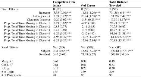
In addition to the variables used in clustering, three additional trial-level variables will be
used as outcome variables in the fourth stage of the analysis to test the predictive utility of the
clusters: trial completion time, number of errors (discrete number of times contacting the course
boundary), and the total distance traveled.
RESULTS Model Generation
Four variables were evaluated for their contribution to movement strategies: At least one
of two movement variables (move time and post-move wait time; see Table 1) crossed with two
context variables (temporal sensitivity and workload; see Table 2). These variable sets were
modeled as Gaussian Mixtures, using the mclust 5 (Fraley & Raftery, 1999, 2003, 2006; Fraley
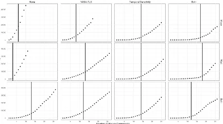
et al., 2012; Scrucca et al., 2016) R package (R Core Team, 2018). Figure 2 shows the entire
model building and evaluation process.
Table 1. Movement Variable Sets to be Used in Clustering.
Clustering Variables Move Wait Move & Wait
Move Time* ✓ ✓
Wait Time* ✓ ✓
Note: Random noise was added to the move time and wait time for each observation, between -1/120th and +1/120th sec., to discourage the clustering procedure from clustering around the framerate of 60 frames per second.
Table 2. Trial-Level Variable Sets to be Used in Clustering.
Clustering Variables None TLX Temporal Sensitivity Both
NASA-TLX ✓ ✓
Temporal Sensitivity ✓ ✓
Each Gaussian Mixture consisted of anywhere between 1 and 26 mixture components,
using the V hyperparameters for the univariate variable sets and the VVV hyperparameters for
the multivariate variable sets. GMMs were fit using MAP estimation. For each of the twelve
variable sets, the modeling procedure was repeated 50 times (600 total runs) using a different
stratified random sample of the data. The samples were stratified on trials, such that movements
set. Each run randomly sampled 405 trials. They were sampled without replacement within a run.
The remaining trials were held out from the clustering procedure, to be used in the test set if that
specific run was selected.
The default mclust initialization procedure was altered to increase the representation of
less frequent but longer events. The initialization for mclust uses hierarchical agglomerative
clustering, which samples a maximum of 2000 events from the training set. Although this
number can be increased, anything much larger exceeds computational limits. Given that each
training data set had approximately 45,000 events, less frequent but longer events (i.e. long
moves) were much less likely to be used in the model initialization, increasing the likelihood that
the specific model converged to a local maximum. To account for this, the initialization used a
weighted sampling procedure, where the likelihood of selecting an event was weighted based on
the percentage of the completion time spent moving for that observation. That is, an event that
was 50% of the trials completion time in duration was ten times as likely to be sampled relative
to an event that was 5% of the trial’s completion time. By repeating this procedure 50 times per
variable set, we were able to average out the effects of any one random subsample.
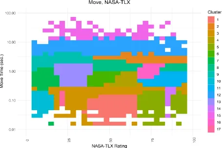
Model Selection
As can be seen in Figure 3, including the NASA-TLX as a modeling variable leads to
decreases in model fit, as measured by BIC, relative to all other models. Similarly, including
both moves and waits decreased model fit relative to all other models. As such, both sets of
models will be omitted from further discussion. Comprehensive analysis of all variable sets,
including those dropped from further discussion, can be found in Appendix 1 through 12 (see
Figure 2. Model Building and Analysis Process.
Table 3. Appendix and Page Number for Variable Set Analysis.
Variable Set Appendix Page
Move Wait NASA-TLX Temporal Sensitivity
✓ 1.1 51
✓ ✓ 1.2 60
✓ ✓ ✓ 1.3 69
✓ ✓ 1.4 84
✓ ✓ 1.5 93
✓ ✓ ✓ 1.6 102
✓ ✓ ✓ ✓ 1.7 117
✓ ✓ ✓ 1.8 141
✓ 1.9 156
✓ ✓ 1.10 165
✓ ✓ ✓ 1.11 174
✓ ✓ 1.12 189
After fitting the mixture components, the mixture components were collapsed into
clusters following the procedure in Baudry et al. (2010). The number of clusters was selected
using a two-piece piecewise linear regression function on the entropy-by-components graph. The
breakpoint in the piecewise regression was selected as the final number of clusters, derived from
combining iteratively the mixture components. Figure 4 shows the entropy plot for the final run
selected from each variable set, as well as the breakpoint for the piecewise linear regression
Table 4. Summary of all 600 runs.
Variables # of Mixture Components # of Clusters BIC
Percentile 25th 50th 75th 25th 50th 75th 25th 50th 75th
M 10 12 14 4 6 7 -31238.40 -28312.80 -25300.40
M, TLX 22 23.5 26 12 14 15.75 -448242.00 -440387.00 -432192.00
M, TLX, TS 25.25 26 26 16 16 17.75 -333819.00 -326600.00 -320465.00
M, TS 24 26 26 14 15 16 25777.92 39484.45 51516.26.00
M, W 25 26 26 12 13 14 -56447.20 -52521.80 -49315.50
M, W, TLX 25 26 26 11 12 13 -471637.00 -466419.00 -458837.00
M, W, TLX, TS 25.25 26 26 14 15 16 -388344.00 -375355.00 -366557.00
M, W, TS 25 26 26 13 14 14.75 -6998.60 7182.841 17978.87
W 9 9.5 10 3 3 3 -36157.60 -34572.20 -33433.30
W, TLX 24 25.5 26 10 12 14 -446819.00 -440016.00 -431010.00
W, TLX, TS 25 26 26 13 15 16 -349321.00 -342420.00 -330657.00
W, TS 24.25 26 26 14 14 16 24750.03 32595.02 39810.41
Table 4, whereas temporal sensitivity improved model fit, the vast majority of models including temporal sensitivity contained more than 12 clusters. The univariate models of
Move-Only and Wait-Move-Only had comparatively fewer clusters, with a median of six and three clusters,
respectively. In line with the stated goal of finding the most parsimonious solution, models with
temporal sensitivity will be dropped from further discussion (see appendices for analysis related
to models using temporal sensitivity). Along similar lines as above, simultaneously including
both moves and waits in the model decreased parsimony (as well as failed the step 2 check in
varying with latency). The univariate models (Move-Only and Wait-Only) were retained for
further discussion.
To select a representative run from each variable set, we used an unconventional
approach. Classically, the “best” model is the model with the highest BIC1 (Steele & Raftery, 2009). However, BIC-based model comparisons rely on both models being applied to samples of
the same size, as the penalty to the log-likelihood scales with the sample size. The repeated
stratified subsampling procedure occurred at the trial level, resulting in models having different
observation counts, and therefore different log-likelihood penalties. Instead, we selected the
model that is the most similar to all other models, as measured by the Adjusted Rand Index
(ARI). The Adjusted Rand Index measures the degree of similarity between two cluster
solutions. It does this by looking at the degree to which pairs of values are in the same cluster in
both clustering solutions, correcting for chance pairings. It ranges from approximately 0 to 1
(Hubert & Arabie, 1985; Rand, 1971).
For each variable set, each of the 50 runs was applied to each specific run’s training
subsample (leading to a 50 by 50 matrix), and an ARI for each pairing was derived. The run
with the highest median ARI across all training samples was selected to represent the overall
variable set.
Table 5 shows the final model selected for each candidate variable set, along with the number of clusters, the number of mixture components, the BIC for the training set, and the
median ARI. Descriptives for both the mixture components and clusters can be found in the
related appendices (see Table 3). The selected run for the Move-Only Cluster solution can be
seen in Table 6 and Figure 5. The selected run for the Wait-Only cluster solution can be seen in
Table 5. Summary of final candidate models.
Variables Appendix # of Clusters # of Mixtures BIC # of Obs. Median ARI
M 1 6 10 -33180 46771 0.81
M, TLX 2 8 17 -441911 47398 0.54
M, TLX, TS 3 17 26 -309107 50937 0.54
M, TS 4 14 25 20069.17 46370 0.72
M, W 5 13 26 -58853.2 46516 0.89
M, W, TLX 6 12 26 -484171 50548 0.72
M, W, TLX, TS 7 12 26 -367947 50585 0.67
M, W, TS 8 14 25 1696.89 47529 0.71
W 9 3 11 -33579.8 47864 0.98
W, TLX 10 13 26 -441684 46607 0.43
W, TLX, TS 11 18 25 -359523 51484 0.55
W, TS 12 14 26 39068.54 52210 0.63
Note: M - Move, TLX - NASA TLX, TS - Temporal Sensitivity, and W – Wait
Table 6. Cluster Summary for Move-Only Solution.
Cluster Move (sec) Wait (sec) NASA-TLX
Temporal Sen.
Prop. Obs. in Training
Prop. Time in Training
1 0.12 (0.04) 0.47 0.04
2 0.28 (0.04) 0.09 0.02
3 0.46 (0.07) 0.09 0.03
4 1.05 (0.34) 0.28 0.20
5 3.10 (0.80) 0.05 0.11
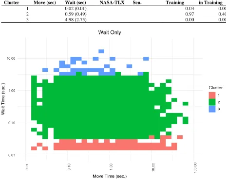
Table 7. Cluster Summary for Wait-Only Solution.
Cluster Move (sec) Wait (sec) NASA-TLX
Temporal Sen.
Prop. Obs. in Training
Prop. Time in Training
1 0.02 (0.01) 0.03 0.00
2 0.59 (0.49) 0.97 0.40
3 4.98 (2.75) 0.00 0.00
Figure 6. Observations with Assigned Clusters (Combined) for Wait-Only Solution.
Evaluating Cluster Solutions
At this stage of analysis, the chosen model parameters were used to analyze the test data.
To support that cluster solutions were coalescing around movement strategies, a χ2-like test was used, measuring the relationship between latency and mean cluster frequency. This approach
uses a Monte Carlo simulation to create a null distribution from the marginal values, randomly
generating a series of contingency tables and their associated χ2 values. The χ2 for the observed
describe how much more extreme the observed contingency table is relative to the null
distribution generated from 10,000,000.
Table 8. Mean Freq. of Cluster for Move-Only Cluster Solution
Cluster Latency
Marginal Means
0 125 250 375 500 625 750 875 1000
1 50.33 16.79 12.02 29.14 40.74 78.21 101.61 133.41 82.07 60.48
2 9.43 6.42 4.54 7.21 8.52 12.30 15.09 14.84 20.07 10.94
3 7.65 8.05 5.07 7.28 9.45 12.47 13.84 16.07 18.66 10.95
4 14.2 17.76 17.39 29.84 33.00 40.05 38.16 42.09 47.48 31.11
5 3.58 3.87 4.12 4.51 6.05 7.60 7.48 6.07 7.80 5.67
6 2.05 1.71 2.41 1.86 2.17 1.91 2.00 1.73 1.45 1.92
Marginal Means 14.54 9.10 7.59 13.31 16.65 25.42 29.70 35.70 29.59 20.18
ꭓ2 = 60.11, p =.02
Table 9. Mean Freq. of Cluster for Wait-Only Cluster Solution
Cluster Latency
Marginal Means
0 125 250 375 500 625 750 875 1000
1 4.92 4.50 3.93 3.58 3.36 3.02 2.98 2.57 2.48 3.48
2 56.40 45.18 50.12 68.70 87.71 154.19 171.36 212.75 183.23 114.41
3 0.02 0.00 0.05 0.05 0.05 0.12 0.07 0.23 0.30 0.1
Marginal Means 20.45 16.56 18.03 24.11 30.37 52.44 58.14 71.85 62.00 39.33
ꭓ2 = 22.48, p =.007
The cluster assignments for both the Move-Only (χ2 = 60.11, p =.02; Table 8) and Wait-Only cluster solutions (ꭓ2 = 22.48, p =.007; Table 9) were not independent of latency, supporting
that those cluster solutions were capturing an element of movement strategy. However, as can be
seen in Table 7 and Table 9, Cluster 2 of the Wait-Only cluster solution contained the vast majority of observations (97%) and trial time (40% compared to <1% for both 1 and 3). This
lessens the practical significance of that cluster solution, and the Wait-Only solution will be
dropped from further discussion. Analysis related to the Wait-Only solution, such as the
Understanding Movement Patterns with the PRONET Technique
Following the PRONET technique, transition matrices between clusters for the remaining
cluster solution (Move-Only) were passed to a Pathfinder analysis (Schvaneveldt, Durso, &
Dearholt, 1989), using the R comato (Muehlin, 2018) and igraph (Csardi & Nepusz, 2006)
packages. Transition matrices used raw frequencies, as we are interested in the overall strategy
differences, rather than parsing out the effects of the initial condition. Pathfinder network
parameters were set to minimize the overall structure (fewest links), which occurs when q = n -1
and r = ∞.
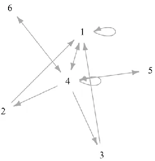
Figure 7 shows a Pathfinder network of the transitions between clusters for the
Move-Only cluster solution. The network structure of these clusters is indicative of a continuous move
strategy found at low latencies, characterized by the Cluster 6 (M = 9.62 sec, SD = 6.60) to
Cluster 4 (M = 1.05 sec, SD = 0.34) cycle (6→4 cycle). The network structure is also indicative
of the classic Move and Wait strategy, characterized by the Cluster 5 (M = 3.10 sec, SD = 0.80)
to Cluster 4 (M = 1.05 sec, SD = 0.34) cycle (5→4 cycle) and the Cluster 4 to Cluster 4 cycle
(4→4 cycle). These cycles are indicative of the classic Move and Wait strategy given the
relatively moderate movement times of Clusters 5 and 4 and their rapid increase in frequency as
a function of latency (see Table 8).
There are also a set of cycles (2 / 3 →1 →4; 1→1; 1→4) typified by much shorter and
more frequent movements (Cluster 1, M = 0.12 sec, SD = 0.04; Cluster 2, M = 0.28 sec, SD =
0.04; Cluster 3, M = 0.46 sec, SD = 0.07). These cycles support the existence of a Staccato
strategy (or strategies), where participants are rapidly pressing a single button. This may be the
equivalent of the slower cursor drag seen in Hoffman et al. (2018). This equivalency is supported
133.41 at .875 sec -- followed by a drop-off down to 82.07 at 1 second. That is, cycles typified
by Cluster 1 are likely to be intermediary strategies existing between continuous and discrete
movements, such as the Staccato strategy. The 2 →1 and 3 →1 links may actually represent an
acceleration button press, given that they exit directly to Cluster 1 and that both have very low
counts (both at 9% of all observations) and extremely low proportion of total time (2% and 3%
respectively). Given their ancillary role in the overall Staccato strategy represented by the 4→2 /
3 →1→1 and 1→1 cycles, discussion about these will be subsumed into the overall discussion
on the Staccato strategy.
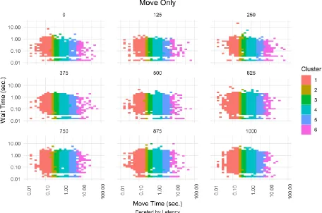
The changes from Figure 7 to Figure 8 (.5 sec) and Figure 8 (1 sec) further support the
role of Cluster 1 as an indicator of a Staccato strategy and Cluster 5 as an indicator of a Move
and Wait strategy, respectively. This is highlighted by the change of the 4 →5 link at 0.5 sec of
latency (see Figure 8, middle panel) to 1→5 at 1 sec of latency (see Figure 8, right panel). Given
that the Staccato strategy is likely an intermediary between the continuous movement strategy
typified by the 6→4 link and the Move and Wait strategy typified by the 5→4 link, it’s logical
that the Staccato strategy and Move and Wait strategy become more connected at higher
latencies through the 1→5 link.
Figure 8. Pathfinder Network of Cluster Transitions (Frequency) for Move-Only Solution, Subset by Latency
Cluster 4 acts as a central node (Gillan, Breedin & Cooke, 1992) between these longer
movements and the much shorter movements, suggesting a central role across all movement
strategies. Given its moderate duration, high frequency across latencies, and close relationship to
the continuous movement (Cluster 6), shorter Move-and-Wait movement (Cluster 5) and
rapid-fire Staccato move (Cluster 1), Cluster 4 may be indicative of a strategy invariant, existing across
the central region of the map requires zigzag movements whose length approximately match the
duration of Cluster 4. Figure 8 supports this view of Cluster 4 as an invariant, either due to a
strategy invariant or route artifact. Figure 8A shows that Cluster 6 (long move) cycles with
Cluster 4, linking the longer continuous movement with the shorter, 1-second movements.
Cluster 4, in this role, may be indicative of course adjustments while Cluster 6 is a likely
indicator of a continuous movement strategy.
Figure 9. Change in Frequency-Based Pathfinder Network Similarity.
Figure 9 compares the Pathfinder networks constructed from the transition matrix, subset
at each latency, with the subsequent latency. The network similarity score is a measure of the
number of links in common between two networks, ranging from 0 for no shared links to 1 when