8. Image Quality Process With Internal Generative Mechanism

Image Quality Process With Internal Generative Mechanism

Kayitha Jaswanth Raju, B.Nihar Assistant Professor Prasad Engineering College

(1)

, Dept. of ECE, Prasad Engineering College

(2

I. INTRODUCTION

SINCE the human visual system (HVS) is the ultimate receiver of sensory information, perceptual image quality assessment (IQA) is useful for many image and video systems, e.g., for information acquisition, compression, transmission and restoration, to make them HVS oriented. The subjective evaluation is the most reliable way for IQA; however it is too cumbersome and expensive to be used in computational information processing systems. Therefore, an objective visual quality metric consistent with the subjective perception is in demand.

Manuscript received January 13, 2012; revised July 18, 2012; accepted August 5, 2012. Date of publication August 17, 2012; date of current version December 20, 2012. This work was supported by the Singapore Ministry of Education Academic Research Fund Tier 2 under Grant T208B1218 and the National Science Foundation of China under Grant 61033004, Grant 61070138, Grant 61072104, and Grant 61227004. The associate editor coor-dinating the review of this manuscript and approving it for publication was Dr. Stefan Winkler.

J. Wu and G. Shi are with the Key Laboratory of Intelligent Perception and Image Understanding of the Ministry of Education of China, School of Electronic Engineering, Xidian University, Xi’an 710071, China (e-mail: [email protected]; [email protected]).

W. Lin and A. Liu are with the School of Computer Engineering, Nanyang Technological University, 639798 Singapore (e-mail: [email protected]; [email protected]).

Color versions of one or more of the figures in this paper are available online at http://ieeexplore.ieee.org.

Digital Object Identifier 10.1109/TIP.2012.2214048

The simplest IQA metrics are the mean-square-error (MSE) and its corresponding peak signal-to-noise ratio (PSNR), which directly compute the error on the intensity of images. They are the natural way to define the energy of the error signal [1]. However, these two metrics consider nothing about the characteristic of the original signal. As a result, they do not always agree with the subjective quality perception, though they are good for content-independent noise [2] (e.g., additive noise [3]).

In order to develop an accurate IQA metric in accord with the subjective perception, researchers turn to investigate the HVS characteristics to seek for image features which affect quality assessment, such as brightness, contrast, frequency content, structure and statistical information [4]. Many HVS oriented IQA

ABSTRACT

: Objective image quality assessment (IQA) aims to evaluate image quality consistently with human perception. Most of the existing perceptual IQA metrics cannot accurately represent the degradations from different types of distortion, e.g., existing structural similarity metrics perform well on dependent distortions while not as well as peak signal-to-noise ratio (PSNR) on content-independent distortions. In this paper, we integrate the merits of the existing IQA metrics with the guide of the recently revealed internal generative mechanism (IGM). The IGM indicates that the human visual system actively predicts sensory information and tries to avoid residual uncertainty for image perception and understanding. Inspired by the IGM theory, we adopt an autoregressive prediction algorithm to decompose an input scene into two portions, the predicted portion with the predicted visual content and the disorderly portion with the residual content. Distortions on the predicted portion degrade the primary visual information, and structural similarity procedures are employed to measure its degradation; distortions on the disorderly portion mainly change the uncertain information and the PNSR is employed for it. Finally, according to the noise energy deployment on the two portions, we combine the two evaluation results to acquire the overall quality score. Experimental results on six publicly available databases demonstrate that the proposed metric is comparable with the state-of-the-art quality metrics.

Of Advanced Research in Engineering & Management (IJAREM)

metrics have been pro-posed during the recent ten years, such as noise quality measure (NQM) [5], structural similarity (SSIM) [6], visual information fidelity (VIF) [7], the PSNR-HVS-M [8], visual signal-to-noise ratio (VSNR) [9], and the recently proposed most apparent distortion (MAD) [10] and feature similarity (FSIM) [11].

The SSIM index is the most popular one among all of these IQA metrics. This index is based on the assumption that the HVS is highly adapted for extracting structural information from the input scene [6]. In [12], [13], SSIM is improved by using edge/gradient feature of the image since the edge conveys important visual information for understanding. In addition, as another high-level HVS property based and well accepted metric, the VIF index computes the mutual information between the reference and test images for visual information fidelity evaluation [7]. These HVS oriented IQA metrics promote our understanding on sensory signal processing and perceptual quality assessment.

Different types of distortion cause different degradation. However, these existing HVS oriented IQA metrics mainly consider the content-dependent characteristics (e.g., structure in SSIM metric, gradient in GSIM metric) in their evaluation. As a result, these HVS oriented IQA metrics perform well on content-dependent distortions (e.g., blur and compression noise) but not well enough on content-independent distortions (e.g., white noise and impulse noise) [3]. While PSNR/MSE performs the opposite way. Recently, Larson and Chandler [10] advocated that the HVS uses multiple strategies to determine image quality. And near-threshold and clearly visible (suprathreshold) distortions are measured separately in their model. This model mainly considers the distinctions of different energy levels rather than the different effects of distortions. In [14], Li et al. introduced an ad hoc procedure to decouple the original distortion into detail loss and additive impairment for discriminative measurement. However, the decomposition for distortions is not well grounded and the performance improvement is limited (which will be further analyzed in Subsection IV-A).

Recent researches on brain theory and neuroscience, such as the Bayesian brain theory [15] and the free-energy principle [16], indicate that the brain works with an internal generative mechanism (IGM) for visual information perception and understanding. Within the IGM, the brain performs as an inference system that actively predicts the visual sensation and avoids the residual uncertainty/disorder [15]–[17]. Thus, we adopt a Bayesian prediction model [15], [18] in our method, and the input scene is decomposed into predicted and disorderly portions. We suppose that distortions on the predicted content will damage the primary visual information, such as blur the edge and destroy the structure, which impact on image understanding. Therefore, edge and structure similarity [6], [12] are used for evaluation on this portion. On the other hand, distortions on the disorderly portion (predicted residual, which arouses uncomfortable sensation) is somewhat content-independent. Therefore, we adopt the PSNR to estimate the degradation on disorderly uncertainty since PSNR is good for content-independent noise measurement [1], [3]. Finally, we combine the results on the two portions with an adaptive nonlinear procedure to acquire the overall score. Experimental results on six publicly available image databases confirm that the proposed model is comparable with the state-of-the-art IQA metrics.

The rest of this paper is organized as follows. In Section II, we further explain the motivation of the proposed model. The detailed implementation of the proposed perceptual quality metric is presented in Section III. Then, in Section IV the performance of the proposed metric is demonstrated. Finally, we draw the conclusions in Section V.

II. MOTIVATION

In this section, we firstly give a brief introduction about the recent brain theory on visual sensation processing, i.e., the internal generative mechanism (IGM) of the brain. Then, according to the IGM theory, we analyze the individual degradations of two representative types of distortion.

FIG:1. Effects of different types of distortion (awgn and gblur). Images are from the TID database [24]. Results for four MSE levels (27, 58, 112, and 225) are demonstrated with 25 different images used for each level. The mean and variance values of the MOS for the images in each level are indicated by points and their corresponding bars.

According to the active inference procedure in the IGM mentioned above, we decompose an input scene into two portions, which we call the predicted portion and the disor-derly portion. The predicted portion derives from the active inference of the input scene, and it possesses the primary visual information (e.g., edge and structure) which will be transmitted into the high-level of the HVS for image under-standing and recognition [23]. While the disorderly portion is composed of the residual uncertainty which the HVS tries to avoid [16]. We believe that the visual contents in the two portions play different roles: distortions on the predicted portion degrade the primary visual information (e.g., blur the edge and structure), and they will directly impact on image understanding; meanwhile, distortions on the disorderly portion mainly change the disorder/uncertainty of the original image, which do not disturb the inference of the primary visual information and mainly arouse uncomfortable perception.

Of Advanced Research in Engineering & Management (IJAREM)

(a) (b) (c)

(d) (e)

Fig. 2. Visual comparison (with the Sailboat image [24]) the effects of awgn and gblur distortions. (a) Reference image. (b) and (c) White noise contaminated images. (d) and (e) Blurred images.

The missing visual content is unable to be predicted by the IGM and the reconstructed image in the HVS is much different from the original undistorted image. Furthermore, as shown in Fig. 1, the quality difference between the two distortions becomes larger when the error energy increases. Notice that the two types of distortion have similar perceptual quality when the error energy is small (i.e., the first points of the two types of distortion in Fig. 1 with high quality score). It is expected since noise will be masked by the image itself (regardless what type of distortion it is) if the noise is smaller than a threshold [27], [28].

An intuitive example is given in Fig. 2. The error energies in Fig. 2(b) (MSE = 29) and (d) (MSE = 28) are small, and therefore both of the contaminated images have high quality score (the MOS (the higher the better) values of Fig. 2(b) and (d) are 5.70 and 5.30, respectively). While under a high level of error energy, the awgn contaminated image (Fig. 2(c) with MSE = 229 and MOS = 4.06) has a much higher perceptual quality than the gblur contaminated image (Fig. 2(e) with MSE = 267 and MOS = 2.52). Note that though Fig. 2(c) is rough, the HVS can still predict most of the visual content the same as that in Fig. 2(a). In other words, the awgn distortion in Fig. 2(c) mainly arouses uncomfortable sensation, and has limited effect on image understanding. On the contrary, the gblur distortion in Fig. 2(e) severely degrades the primary visual information and the HVS can hardly accurately predict the objects (such as the people in the figure). In summary, different types of distortion generate different effects on primary visual information and disorderly uncertainty, which result in different degradations on quality. Furthermore, under a same error energy level, the distortion which mainly affects the inference of the primary visual information generates more quality degradation than that changes the disorderly uncertainty.

Therefore, according to the above discussions, the individual degradation from different types of distortion can be represented by the degradations on the two decomposed portions. In this paper, considering the effects of the distortions, we adopt different measurements to separately evaluate the primary visual information degradation and disorderly uncertainty degradation for perceptual quality assessment. Detailed implementation will be given in the next section.

III. PROPOSED IQA SCHEME

model. Then degradations on the two portions are evaluated respectively. Finally, we combine the results of the two portions based on error energies distribution to deduce the overall perceptual quality score. The flowchart of the proposed model is shown in Fig. 3.

A. AR Based Image Prediction

Image decomposition is an effective image processing tool [14], [29], [30], which splits an image into two or more portions for discriminately processing, e.g., to decompose an input scene into textural and cartoon parts for just noticeable difference estimation [28]. In this paper, inspired by the IGM theory about the visual perceptual process, we try to decompose an image into predicted and disorderly portions for quality evaluation. Since the Bayesian brain theory indicates that the brain performs as an active inference procedure [16], [31], we adopt a Bayesian prediction based autoregressive (AR) model [18], [32] for image content inference

Figure: 3. Flowchart of the proposed model𝑰𝒓_{, 𝑰}𝒕 _{is the reference image, 𝑰} 𝑫 𝒓_(𝑰

𝑫 𝒕_{) and 𝑰}

𝒅 𝒓_(𝑰

𝒅

𝒕_{) are the predicted}

and disorderly portions of 𝑰𝒓_(𝑰𝒕_{), respectively.}

The Bayesian brain theory uses Bayesian probability to imitate the inference procedure for image perception and understanding in the IGM [15], [16]. The key of this theory is a probabilistic model that optimizes the input scene by minimizing the prediction error. For example, with an input scene, the Bayesian brain system tries to maximize the conditional probability p(x/X) between the central pixel x and its surrounding X= {x1,x2, . . . ,xN} [15] for error minimization.

By decomposing the conditional probability p(x/X) and analyzing the correlation between the central pixel x and the pixels xi in the surrounding X , it can be seen that these xi which strongly correlated to x play

dominant roles for p(x /X)maximization [33]. Therefore, the mutual information (I(x;xi)) between the central

pixel x and its surrounding pixel xi is adopted as the autoregressive coefficient, and an AR model is created to

Of Advanced Research in Engineering & Management (IJAREM)

𝒙′_{= 𝑪𝒊𝑿𝒊}

𝒙_{𝒊 ∈𝑿} + 𝜺 (1)

where x_ is the predicted value of pixel x, Ci = I (x;xi ) / I(𝑥; 𝑥𝑘)_𝑘 being the normalized coefficient, and ε is white noise. In this paper, we set X as a 21 × 21 surrounding region. With the predicted model (1), an input image (I ) is decomposed into two portions, the predicted image (Ip ) and the disorderly image (Id ), as

shown in Fig. 4. In the next subsections, we will evaluate the degradations on the two decomposed images, respectively, since distortions on the two portions have different impacts toward the perceptual quality.

B. Uncomfortable Sensation Variation

The disorderly portion is composed of the uncertain stimuli of the original image [16]. Distortion on this portion has little effect on image understanding and mainly generates uncomfortable sensation. As a natural way to define the energy of the error signal [1], the PSNR metric presents a good match with the HVS when the error signal is independent of the original signal [3], and this point is also confirmed by the experiments in [2]. Since the distortion of the disorderly portion is independent of the original image content, the PSNR is adopted to evaluate the quality of this portion. Therefore the uncomfortable sensation variation is computed as follow

𝑷 𝑰𝒅𝒓, 𝑰𝒅𝒕 = 𝟏 𝑪𝟏

𝒑𝒔𝒏𝒓 𝑰𝒅𝒓, 𝑰𝒅𝒕 = 𝟏 𝑪𝟏

𝟏𝟎 𝐥𝐨𝐠𝟏𝟎

𝟐𝟓𝟓𝟐

MSE 𝑰_𝒅𝒓_{, 𝑰} 𝒅

𝒕 (𝟐)

where 𝑰𝒅𝒓 and 𝑰𝒅𝒕 are the disorderly portions of the reference and test images, respectively; psnr(𝑰𝒅𝒓 , 𝑰𝒅𝒕)

is the PSNR value between 𝑰𝒅𝒓 and 𝑰𝒅𝒕 , and MSE(𝑰𝒅𝒓 , 𝑰𝒅𝒕) is the mean squared error between 𝑰𝒅𝒓 and 𝑰𝒅𝒕 (the

minimal value of MSE (such as 1) is set to avoid infinite psnr); 𝑪𝟏 is a constant parameter which is used to normalize the PSNR value into the range [0 1], for this purpose, we set 𝐶1= 10 log102552

C. Visual Information Degradation

Since the predicted portion possesses the primary visual information and distortion on this portion impacts on image understanding, we should adopt some high-level HVS proper-ties to evaluate the degradation of the visual information. In this paper, degradations on edge and structure are computed for primary visual information fidelity evaluation.

The HVS is highly sensitive to the edge, which conveys important visual information and is crucial for scene under-standing [12], [34]. The degradation on the edge between the predicted portions of the reference image (Ipr ) and the test image (Ipt ) is computed as their edge height similarity,

𝒈 𝒙𝝆, 𝒚𝝆 = 𝟐𝑬𝒑

𝒓_(𝒙

𝝆)𝑬𝒑𝒕(𝒚𝝆) + 𝑪𝟐 𝑬𝒑𝒓(𝒙𝝆)𝟐+ 𝑬𝒑𝒓(𝒚𝝆)𝟐+ 𝑪𝟐

(𝟑)

where 𝒙𝝆 and 𝒚𝝆 are the corresponding pixels from the predicted portions of the reference and test images (𝑰𝝆𝒓 and 𝑰𝝆𝒕 ), respectively; g(𝒙𝝆,𝒚𝝆) is the edge similarity between 𝒙𝝆 and 𝒚𝝆, 𝑬𝝆𝒓 and 𝑬𝝆𝒕 are the edge

height maps of 𝑰𝝆𝒓 _{and 𝑰𝝆}𝒕 _{respectively, C2 is the small constant to avoid the denominator being zero and is set as}

C2 = (0.03 × L)2 , and L is the gray level of the image.

The edge height 𝑬𝝆𝒓 (same for𝑬𝝆𝒕) is computed as the maximal edge response along the four directions,

Fig. 5. Edge filters for four directions. (a) Horizontal. (b) 45 degrees (c) 135 degrees. (d) Vertical.

𝑬𝒑𝒓 𝒙 = 𝒎𝒂𝒙 𝑮𝒓𝒂𝒅𝒌(𝒙𝒑) (𝟒) 𝑮𝒓𝒂𝒅𝒌= (𝝋𝛁𝒌∗ 𝑰𝒑𝒓 _(𝟓)

where ∇k are four directional filters, as shown in Fig. 5, ϕ = 1/16, and symbol ∗ denotes the convolution operation.

However, some image regions (e.g.,the feather of the parrots in Fig. 4) has no apparent edge but still represents specific structural character. In addition, the HVS is highly adapted for extracting structural information from a scene for recognition. Therefore, besides edge similarity, we need another primary visual information degradation measurement to evaluate the fidelity on image structure. Here, we adopt the structural similarity [6] to evaluate the degradation on structural information

𝒔 𝒙𝝆, 𝒚𝝆 =

𝟐𝝈𝒙𝝆𝒚𝝆+ 𝑪𝟑 𝝈𝒙𝝆

𝟐 _{+ 𝝈} 𝒚𝝆 𝟐 _{+ 𝑪}

𝟑

(𝟔)

Where𝑠(𝑥𝜌, 𝑦𝜌)is the structural similarity between patches(𝐵(𝑥𝜌) and 𝐵(𝑦𝜌))entered at

𝑥𝜌and 𝑦𝜌 ; 𝜎𝑥𝜌𝑦𝜌is the covariance of the two patches; 𝝈𝒙𝝆 𝟐 _(𝝈

𝒚𝝆

𝟐 _{) is the variance of the patch𝐵 𝑥}

𝜌 𝐵 𝑦𝜌 ;we

set the patch size as 11 × 11,and the constant 𝐶3= 𝐶2

2(the same as in [6]).

Combining the edge and structure similarities, we deduce the degradation on primary visual information as

𝒗 𝒙𝝆, 𝒚𝝆 = 𝒈 𝒙𝝆, 𝒚𝝆 𝒔 𝒙𝝆, 𝒚𝝆 (𝟕)

D. Overall Perceptual Quality

Distortions on the two portions codetermine the quality of the contaminated image. The distortion on the disorderly portion degrades image quality by disturbing our attention and arousing uncomfortable sensation. On the other hand, the distortion on the predicted portion changes the original visual content and affects image understanding. Therefore, we combine the evaluation of the two portions, (2) and (7), to acquire the perceptual quality score

𝑸 = 𝑷𝜶_𝑽𝜷_(𝟖)

Where V is the pooling value of the predicted portion (mean value of all 𝑣 𝑥𝜌, 𝑦𝜌 ); the parameters α and β are used to adjust the relative importance of the two portions.

The weights of the two evaluation parts, P and V, are closely related to the noise energy level on the two decomposed portions. The more noise energy that one decomposed portion possesses, the more important role it will play. For example, if most of the noise is in the disorderly portion, the noise mainly arouses uncomfortable sensation and the uncomfortable sensation variation is dominant in the quality assessment. Thus a big value of α is required in (8) to highlight the evaluation result of the disorderly portion (P). On the contrary, when the noise is mainly in the predicted portion, the quality degradation is primarily caused by the change of the primary visual information. A big value of β is needed to highlight the evaluation result of the predicted portion (V). According to the analysis above, we compute the importance parameter based on the noise energies of the two portions, and we set

𝜶 = 𝑴𝑺𝑬𝒅

𝑴𝑺𝑬𝒅+ 𝑴𝑺𝑬𝝆

𝟗

Where𝑴𝑺𝑬𝒅is the energy of noise between the disorderly portions of the reference image𝛼 ∈ 0 1 .(Ird) and the test image(Itd );MSEpis the energy of noise between the two predicted images(Irpand Itp), and

Meanwhile, as same as (9),we set𝜷 = 𝑴𝑺𝑬𝝆

𝑴𝑺𝑬𝒅+𝑴𝑺𝑬𝝆= 𝟏 − 𝜶

Moreover, considering the viewing conditions (i.e. the viewing distance and the display resolution), multi-scale evaluation is adopted to deduce the overall quality score

𝑺𝟎= 𝑸𝒊

𝝆𝒊 ⨼

Of Advanced Research in Engineering & Management (IJAREM)

Where Qiis the perceptual quality score on the i th

level based on (8), the parameter ρ defines the relative importance of different scales, and its value is set asp = [0.0448, 0.2856, 0.3001, 0.2363, 0.1333]which is obtained through psychophysical experiment.

IV. EXPERIMENTAL RESULTS

In this section, the effectiveness of the proposed perceptual IQA metric is firstly demonstrated. And then, we analyze the performance of the proposed metric on individual type of distortion. Finally, the proposed metric is compared with the Lates tand / or well-accepted metrics on six publicly available databases. The proposed IQA metric operates on gray image only, the color input is converted to gray image.

To evaluate the performance of the IQA metrics on a common space, a five-parameter mapping function [36] is firstly adopted to nonlinearly regress the computational quality score (S0),

𝑺𝒓= 𝜷𝟏

𝟏

𝟐−

𝟏

𝟏 + exp(𝜷𝟐(𝑺𝟎− 𝜷𝟑))

+ 𝜷𝟒𝑺𝟎+ 𝜷𝟓 (𝟏𝟏)

Where{𝛽1, 𝛽2, 𝛽3, 𝛽4, 𝛽5} are the parameters to be fitted.

(a) (b) (c)

(d) (e) (f)

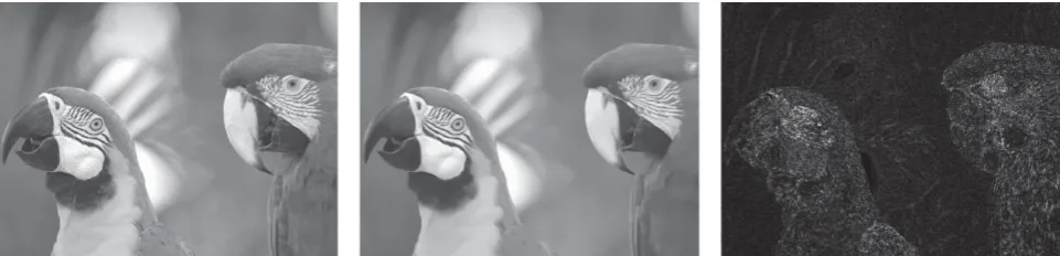
Fig. 6. Demonstration of the effectiveness of the proposed model. The reference image is shown in Fig. 4(a). The first column contains the original images, while the middle and last columns contain the corresponding predicted and disorderly portions, respectively (pixel values of the two disorderly images have been scaled to [0, 255] for a clearer view). (a) Distorted image contaminated by white noise (MSE = 115, MOS = 4.77, MSSIM = 0.9048, VIF = 0.4649, and Proposed = 0.9442). (b) MSEp is eight. (c) MSEd is 96. (d) Distorted image contaminated by JPEG transmission error (MSE = 123, MOS = 3.72, MSSIM = 0.9390, VIF = 0.5326, and Proposed = 0.9236). (e) MSEp is 77. (f) MSEd is 32. The white noise mainly increases the degree of uncomfortable sense and has almost no effect on the primary visual information. The JPEG transmission error (damaging the structure of the feather and blurring the edge of the parrots) obviously changes the primary visual information. Therefore, under the similar energy of noise, (a) has a better quality (higher MOS) value than (d).

Then, the computational scores (Sr) are compared withthe ground truth values (MOS or differential

mean squared error (RMSE), and outlierratio (OR). The first two criteria can measure predictionmonotonicity and the other three are used to evaluate predictionaccuracy [36]. A better IQA metric has higher SRCC,KRCC, and PLCC, while lower RMSE and OR values. Moredetails about the five criteria can be found in [37] and [14].

A. Analysis on the Proposed IQA Metric

The proposed perceptual IQA metric is based on the sen-sory information processing mechanism in the HVS, which separately evaluates the degradation on the primary visual information and the perceptual uncomfortable variation. We make a comparison with two well accepted IQA metrics, the MSSIM [6] and the VIF [7], to demonstrate the effec-tiveness of the proposed metric. In Fig. 6, (a) is the white noise contaminated image and (d) is the JPEG transmission error contaminated image. The reference image is shown in Fig. 4(a).

Fig. 6(a) has a better perceptual quality than Fig. 6(d) (the MOS value of (a) is higher than that of (d)), though the error energies of the two images are similar. That is because the two types of distortions play different roles in the HVS. As stated in Section II, the HVS highly tolerates the white noise, and can effectively filter out this type of noise with the help of the IGM. As a result, the white noise in Fig. 6(a) mainly arouses uncomfortable sense and has little effect on image understanding. While the JPEG transmission error degrades some high-level properties of the image content, i.e., damaging the structure of the left parrot and blurring the edge between the left parrot and the background, which impacts on the image recognition and understanding.

Since most of the existing HVS oriented IQA metrics indis-criminately treat distortions on the image and directly evaluate the visual information degradation, they cannot effectively discriminate the effect of noise on uncomfortable sense or content understanding. As a result, these HVS oriented IQA metrics do not work well enough on the two distorted images. For example, as shown in Fig. 6, according to the MSSIM and VIF metrics, image (a) (with MSSIM = 0.9048 and VIF = 0.4649) has worse quality than (d) (with MSSIM = 0.9390, VIF = 0.5326), which contradicts the subjective quality assessment result.

The proposed IQA metric discriminately treats the two types of distortion based on their effects and accurately evaluates image quality degradation. The proposed model decomposes the test images into two portions with a Bayesian prediction procedure, as shown in Fig. 6 for further processing. Almost all of the white noise in Fig. 6(a) is decomposed into the disor-derly portion (c) (MSEd= 96), and a little into the predicted portion (b) (MSEp= 8). As has been discussed in Section II, the noise in the disorderly portion mainly arouses uncomfort-able sensation and distortion on the predicted portion directly degrades the primary visual information of the original image. Therefore, the decompositions on the white noise is highly in accord with the perception of the HVS. Moreover, most of the JPEG transmission error in Fig. 6(d) is decomposed into the predicted portion (e) (MSEp= 77) (though some structural information is mis-decomposed into the disorderly portion caused by the limitation of the AR model). The proposed IQA metric separately evaluate the degradations on the two decomposed portions to calculate the quality score. As a result, Fig. 6(a) (with pr oposed= 0.9442) has a higher quality score than (d) (with pr oposed= 0.9236), which agrees with the subjective quality assessment results.

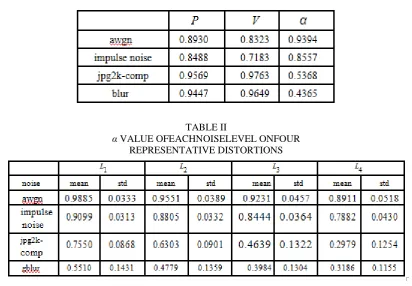
Furthermore, we compare the proposed metric against the ADM metric [14] which also tries to discriminately treat distortions. As shown in Fig. 7, (a) is white noise contaminated image and (b) is JPEG2000 transmission error contaminated image. The white noise in Fig. 7(a) mainly makes the image coarse-grained and changes the structures to some extent (i.e., the structures of the tree and the roof), while has little effect on the edge information. However, the JPEG2000 transmission error severely degrades the original structures and edges, e.g., the artificial masking locates at the top left tree and house of the image. Though the two distorted images with similar error energy (Fig. 7(a) with MSE = 220 and (b) with MSE = 233), Fig. 7(a) (MOS = 4.16) has a better perceptual quality than (b) (MOS = 3.31).

Of Advanced Research in Engineering & Management (IJAREM)

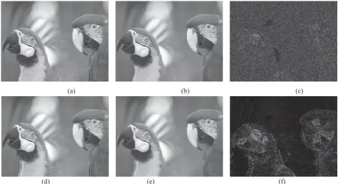
TABLE I

DEMONSTRATION OF EACH COMPONENT OF THE PROPOSED METHOD ON FOUR REPRESENTATIVE DISTORTIONS

TABLE II

α VALUE OFEACHNOISELEVEL ONFOUR REPRESENTATIVE DISTORTIONS

In this experiment, the proposed metric can also accurately evaluate the two distorted images. As shown in Fig 7, a little white noise is decomposed into the predicted portion (d) (MSEp= 49), and this means the white noise has limited effect on the primary visual information. When it comes to the JPEG2000 transmission error distortion, most of the noise which changes the image structure has been decomposed into the predicted portion (f) (MSEp= 104). Moreover, the evaluation results of the proposed metric indicates that Fig. 7(a) (Proposed = 0.9269) has a better perceptual quality than (b) (Proposed = 0.9106). Therefore, the proposed metric is consistent with the HVS.

B. Performance on Individual Distortion Type

In this experiment we analyze the performance of the proposed IQA metric on different types of distortion. Four typical distortion types, including additive Gaussian white noise, impulse noise, JPEG2000 compression, and Gaussian blur, from the TID [24] database (each distortion is with four error energy levels) is chosen to demonstrate the performances of the two evaluators, the uncomfortable sensation variation P in (2) and the primary visual information degradation V in (7). The evaluation results (SRCC values) are listed in Table I. Since the white noise and the impulse noise mainly arouse uncomfortable perception, most of the noise is decomposed into the disorderly portion (with a big α value) and the evaluation result of P is better than that of V . Therefore, the big α value can effectively highlight P for overall quality evaluation on the two distortion types. However, the JPEG2000 compression and blur noise will directly degrade the primary visual information (e.g., change image structure and edge), especially when the error energy is large. And V performs better than P in these two types of distortions.

(a) (b)

(c) (d)

(e) (f)

Of Advanced Research in Engineering & Management (IJAREM)

proposed metric accurately decomposes distortions, thus returning quality scores which is consistent to the HVS.

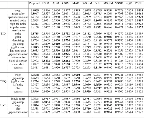
To further demonstrate the effectiveness of the proposed metric on individual distortion type, we make comparison with five latest IQA metrics (FSIM [11], ADM [14], GSIM [12], MAD [10], and IW-SSIM [37]) and another five well accepted IQA metrics (VIF [7], MSSIM [6], VSNR [9], NQM [5], and PSNR). Only the SRCC criterion is used since the other criteria lead to similar conclusions. The experimental results are listed in Table III, where the two best IQA metrics have been highlighted in boldface.

TABLE III

SRCC VALUES OF IQA METRICS FOR EACH DISTORTION TYPE

From Table III we can see that on the TID database, the proposed metric performs the best on the quantization noise, the blur noise, and the two compression noise. Besides, the proposed metric has similar performance with PSNR and outperforms all the other metrics on the two additive noise, the spatial correlated noise and high frequency noise. Furthermore, the proposed metric has similar performance with the best one on impulse noise, denoising noise and the JPEG 2000 transmission error. In summary, on the 13 typical distortion types (the first 13 distortion types of the TID database), the propose metric performs the best on 8 types, close to the best on the remained 5 types. In addition, the proposed metric performs the best on three out of six distortion types on the CSIQ database, and similar with the best results on the remain distortion types. Therefore, the

Proposed FSIM ADM GSIM MAD IWSSIM VIF MSSIM VSNR NQM PSNR

awgn 0.9069 0.8566 0.8630 0.8577 0.8388 0.8028 0.8799 0.8094 0.7728 0.7679 0.9114

awgn-color 0.8947 0.8527 0.8390 0.8091 0.8258 0.8015 0.8785 0.8064 0.7793 0.7490 0.9068

spatial corr-noise 0.9152 0.8483 0.8980 0.8907 0.8678 0.7909 0.8703 0.8195 0.7665 0.7720 0.9229

masked noise 0.7968 0.8021 0.7360 0.7409 0.7336 0.8068 0.8698 0.8155 0.7295 0.7067 0.8487

high-fre-noise 0.9223 0.9093 0.8970 0.8936 0.8864 0.8732 0.9075 0.8685 0.8811 0.9015 0.9323

impulse noise 0.8160 0.7452 0.5120 0.7229 0.6499 0.6579 0.8331 0.6868 0.6471 0.7616 0.9177

TID quantization noise 0.8788 0.8564 0.8500 0.8752 0.8160 0.8182 0.7956 0.8537 0.8270 0.8209 0.8699

gblur 0.9682 0.9472 0.9140 0.9589 0.9197 0.9580 0.9546 0.9607 0.9330 0.8846 0.8682

denoising 0.9704 0.9603 0.9450 0.9724 0.9434 0.9463 0.9189 0.9571 0.9286 0.9450 0.9381

jpg-comp 0.9484 0.9279 0.9410 0.9392 0.9275 0.9181 0.9170 0.9348 0.9174 0.9075 0.9011

jpg2k-comp 0.9845 0.9773 0.9720 0.9759 0.9707 0.9749 0.9713 0.9736 0.9515 0.9532 0.8300

jpg-trans-error 0.8635 0.8708 0.8510 0.8835 0.8661 0.8560 0.8582 0.8736 0.8056 0.7373 0.7665

jpg2k-trans-error 0.8893 0.8544 0.8400 0.8925 0.8394 0.8313 0.8510 0.8525 0.7909 0.7262 0.7765

pattern-noise 0.7295 0.7491 0.8380 0.7372 0.8287 0.7719 0.7608 0.7336 0.5716 0.6800 0.5931

block-distortion 0.7902 0.8492 0.1610 0.8862 0.7970 0.7889 0.8320 0.7617 0.1926 0.2348 0.5852

mean shift 0.4887 0.6720 0.5890 0.7170 0.5161 0.6757 0.5132 0.7374 0.3715 0.5245 0.6974

contrast 0.6411 0.6481 0.4920 0.6737 0.2723 0.6273 0.8190 0.6400 0.4239 0.6191 0.6126

awgn 0.9638 0.9262 0.9583 0.9440 0.9600 0.9380 0.9571 0.9471 0.9241 0.9384 0.9363

jpg-comp 0.9663 0.9654 0.9660 0.9632 0.9660 0.9662 0.9705 0.9622 0.9036 0.9527 0.8882

CSIQ jpg2k-comp 0.9774 0.9685 0.9748 0.9648 0.9770 0.9683 0.9672 0.9691 0.9480 0.9631 0.9363

1/f noise 0.9427 0.9234 0.9488 0.9387 0.9540 0.9059 0.9509 0.9330 0.9084 0.9119 0.9338

blur 0.9724 0.9729 0.9726 0.9589 0.9660 0.9782 0.9747 0.9720 0.9446 0.9584 0.9289

contrast 0.9546 0.9420 0.9508 0.9508 0.9170 0.9539 0.9361 0.9521 0.8700 0.9479 0.8622

jpg2k-comp 0.9675 0.9717 0.9711 0.9587 0.9380 0.9751 0.9654 0.9683 0.9614 0.9100 0.9551

jpg-comp 0.9810 0.9834 0.9790 0.9098 0.9490 0.9645 0.9793 0.9842 0.9764 0.9440 0.9657

LIVE awgn 0.9874 0.9652 0.9820 0.9774 0.9710 0.9667 0.9731 0.9845 0.9694 0.9377 0.9785

blur 0.9538 0.9708 0.9650 0.9517 0.8990 0.9719 0.9584 0.9722 0.9517 0.9649 0.9413

proposed perceptual based IQA metric is highly consistent with the human perception and is comparable with the best IQA metrics.

C. Overall Performance Comparison

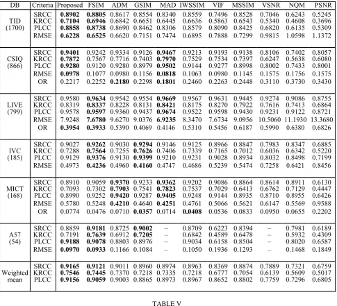
In order to make a comprehensive analysis on the proposed metric, we verify the proposed IQA metric on the overall distortions of the six publicly available databases, TID [24], CSIQ [38], LIVE [39], IVC [40], MICT [41], and A57 [42]. Fig. 8 shows the scatter plots of the evaluation results of the proposed metric on the six databases, which demonstrates the consistence between the proposed metric and the subjective evaluation. Furthermore, we make a comparison with ten IQA metrics. The values of SRCC, KRCC, PLCC, RMAE, and OR are listed in Table IV, where the two best IQA metrics have been highlighted in boldface. Since the standard deviations between the subjects have not been released, the OR is not calculated on the TID, IVC, and A57 databases.

From Table IV, we can see that the proposed IQA metric is the most consistent metric over different databases: it performs the best on the TID, almost the same to the best on the CSIQ and LIVE databases, and only slightly worse than the best on IVC, MICT, and A57 databases. Note that the numbers of the test images (listed in the first column of Table IV) and the distortion types of TID, CSIQ, and LIVE databases are much larger than those of IVC, MICT, and A57, the evaluation results on the first three databases are more convincing than the last three [11]. Therefore, we give the weighted mean (based on the size of these databases) values of SRCC, KRCC and PLCC (weighted mean values of RMSE are not calculated since the ranges of RMSE values are not the same on the six databases) in Table IV.

Furthermore, the statistical significance of the proposed met-ric is evaluated by using F-test which computes the prediction residuals between the IQA metric outputs (after nonlinear mapping) and the subjective scores. Let F denotes the ratio between two residual variances, and Fcr it ical (determined by the number of residuals and the

confidence level) be the judgement threshold. If F>Fcr it ical , then the difference of prediction accuracy between

the two metrics is significant.

(a) (b) (c)

(d) (e) (f)

Fig. 8. Scatter plots of subject scores versus the proposed metric scores for the six databases. (a) TID. (b) CSIQ. (c) LIVE. (d) IVC. (e) MICT. (f) A57.

Of Advanced Research in Engineering & Management (IJAREM)

TABLE IV

PERFORMANCE COMPARISON OF IQA METRICS ON SIX BENCHMARK DATABASES

DB Criteria Proposed FSIM ADM GSIM MAD IWSSIM VIF MSSIM VSNR NQM PSNR

SRCC 0.8902 0.8805 0.8617 0.8554 0.8340 0.8559 0.7496 0.8528 0.7046 0.6243 0.5245

TID KRCC 0.7104 0.6946 0.6842 0.6651 0.6445 0.6636 0.5863 0.6543 0.5340 0.4608 0.3696

(1700) PLCC 0.8858 0.8738 0.8690 0.8462 0.8306 0.8579 0.8090 0.8425 0.6820 0.6135 0.5309

RMSE 0.6228 0.6525 0.6620 0.7151 0.7474 0.6895 0.7888 0.7299 0.9815 1.0598 1.1372

SRCC 0.9401 0.9242 0.9334 0.9126 0.9467 0.9213 0.9193 0.9138 0.8106 0.7402 0.8057

CSIQ KRCC 0.7872 0.7567 0.7716 0.7403 0.7970 0.7529 0.7534 0.7397 0.6247 0.5638 0.6080

(866) PLCC 0.9280 0.9120 0.9280 0.8979 0.9502 0.9144 0.9277 0.8998 0.8002 0.7433 0.8001

RMSE 0.0978 0.1077 0.0980 0.1156 0.0818 0.1063 0.0980 0.1145 0.1575 0.1756 0.1575

OR 0.2217 0.2252 0.2180 0.2298 0.1801 0.2460 0.2263 0.2448 0.3110 0.3730 0.3430

SRCC 0.9580 0.9634 0.9542 0.9554 0.9669 0.9567 0.9631 0.9445 0.9274 0.9086 0.8755

LIVE KRCC 0.8319 0.8337 0.8228 0.8131 0.8421 0.8175 0.8270 0.7922 0.7616 0.7413 0.6864

(799) PLCC 0.9578 0.9597 0.9360 0.9437 0.9674 0.9522 0.9598 0.9430 0.9231 0.9122 0.8721

RMSE 7.9248 7.6780 9.6270 9.0376 6.9235 8.3470 7.6734 9.0956 10.5060 11.1930 13.3680

OR 0.3954 0.3933 0.5390 0.4069 0.4146 0.5310 0.5456 0.6187 0.5990 0.6380 0.6826

SRCC 0.9027 0.9262 0.9030 0.9294 0.9146 0.9125 0.8966 0.8847 0.7983 0.8347 0.6885

IVC KRCC 0.7288 0.7564 0.7255 0.7626 0.7406 0.7339 0.7165 0.7012 0.6036 0.6342 0.5220

(185) PLCC 0.9129 0.9376 0.9130 0.9399 0.9210 0.9231 0.9028 0.8934 0.8032 0.8498 0.7199

RMSE 0.4973 0.4236 0.4960 0.4160 0.4747 0.4686 0.5239 0.5474 0.7258 0.6421 0.8456

SRCC 0.8910 0.9059 0.9370 0.9233 0.9362 0.9202 0.9086 0.8864 0.8614 0.8911 0.6130

MICT KRCC 0.7093 0.7302 0.7903 0.7541 0.7823 0.7537 0.7029 0.6413 0.6762 0.7129 0.4447

(168) PLCC 0.8990 0.9252 0.9420 0.9287 0.9405 0.9248 0.9144 0.8935 0.8710 0.8955 0.6426

RMSE 0.5780 0.5248 0.4210 0.4640 0.4251 0.4761 0.5066 0.5621 0.6147 0.5569 0.9588

OR 0.0774 0.0476 0.0710 0.0357 0.0714 0.0408 0.0536 0.0833 0.0950 0.0655 0.2202

SRCC 0.8859 0.9181 0.8725 0.9002 – 0.8709 0.6223 0.8394 – 0.7981 0.6189

A57 KRCC 0.7191 0.7639 0.6912 0.7205 – 0.6842 0.4589 0.6478 – 0.5932 0.4309

(54) PLCC 0.9188 0.9078 0.8803 0.8976 – 0.9034 0.6158 0.8504 – 0.8020 0.6587

RMSE 0.0970 0.0933 0.1166 0.1084 – 0.1050 0.1936 0.1293 – 0.1468 0.1849

SRCC 0.9165 0.9121 0.9011 0.8960 0.8974 0.8963 0.8369 0.8874 0.7889 0.7321 0.6759

Weighted KRCC 0.7546 0.7445 0.7370 0.7218 0.7335 0.7218 0.6777 0.7054 0.6139 0.5609 0.5017

mean PLCC 0.9156 0.9059 0.9003 0.8865 0.8973 0.8967 0.8652 0.8802 0.7759 0.7296 0.6805

TABLE V

PERFORMANCE COMPARISON WITH F-TEST (STATISTICAL SIGNIFICANCE). THE SYMBOL ―1,‖ ―0,‖ OR ―−1‖ MEANS THAT THE PROPOSED METRIC IS STATISTICALLY (WITH 95% CONFIDENCE)

BETTER, INDISTINGUISHABLE, OR WORSE THAN THE CORRESPONDING METRIC

FSIM ADM GSIM MAD IWSSIM VIF MSSIM VSNR NQM PSNR

TID 1 1 1 1 1 1 1 1 1 1

CSIQ 1 0 1 −1 1 0 1 1 1 1

LIVE 0 1 0 1 1 1 1 1 1 1

IVC −1 0 −1 0 0 0 0 1 1 1

MICT −1 −1 −1 0 −1 −1 0 0 0 1

Table V, the proposed metric performs very well on the three large databases (i.e., TID, CSIQ, and LIVE), especially for the TID database (on which the preposed metric significantly outperforms all other metrics). While the proposed metric performs indistinguishable or worse on the other three small databases, especially for the MICT database. With further analysis we have found that the our AR model performs not very well for the JPEG noise, and cannot accurately decom-pose the distorted image into two portions. The evaluation results of the F-test is much similar with that of the criterion listed in Table IV. In summary, the proposed metric performs state-of-the-art on the three bigger publicly available databases and is highly consistent with the human perception.

V. CONCLUSION

In this paper, we introduce a novel IQA metric by integrating the best existing IQA metrics. SSIM and GSIM perform well on content-dependent distortions but not well enough on content-independent distortions. However PSNR/MSE per-forms the opposite way. Therefore, we try to integrate the merits of these metrics by decomposing the input scene into predicted and disorderly portions, and distortions on these two portions are discriminatively treated. The decomposition is inspired by the recent IGM theory which indicates that the HVS works with an internal inference system for sensory information perception and understanding, i.e., the IGM actively predicts the sensory information and tries to avoid the residual uncertainty/disorder. Since the predicted portion holds the primary visual information and the disorderly portion consists of uncertainty, the distortions on the two portions cause different aspects of quality degradations. Distortions on the predicted portion affect the understanding of the visual content, and that on disorderly portion mainly arouse uncomfortable sensation.

Considering the different properties of the two decomposed portions, we separately evaluate their quality degradations. Firstly, a Bayesian prediction model is adopted to decompose the reference and test images into predicted and disorderly portions, respectively. Then we evaluate the content degradation on their predicted portions with the measurement based on edge and structure similarities, and uncomfortable sensation variation between the disorderly portions of the reference and test images with the PSNR measurement. Finally, according to the noise energy level, we combine the results of the two portions to acquire the overall quality score. Experiments on individual distortion types demonstrate the effectiveness of the proposed metric. Moreover, results on six publicly available databases further confirm that the proposed metric performs consistently with the state-of-the-art IQA metrics.

REFERENCES

[1] Z. Wang and A. C. Bovik, ―Mean squared error: Love it or leave it?‖ IEEE Signal Process. Mag., vol. 26, no. 1, pp. 98–117, Jan. 2009.

[2] Q. Huynh-Thu and M. Ghanbari, ―Scope of validity of PSNR in image/video quality assessment,‖ Electron. Lett., vol. 44, no. 13, pp. 800–801, Jun. 2008.

[3] N. Ponomarenko, V. Lukin, A. Zelensky, K. Egiazarian, M. Carli, and Battisti, ―TID2008—a database for evaluation of full-reference visual quality assessment metrics,‖ Adv. Modern Radioelectron., vol. 10, pp. 30–45, May 2009.

[4] H. R. Sheikh, A. C. Bovik, and G. de Veciana, ―An information fidelity criterion for image quality assessment using natural scene statistics,‖ IEEE Trans. Image Process., vol. 14, no. 12, pp. 2117–2128, Dec. 2005.

[5] N. Damera-Venkata, T. D. Kite, W. S. Geisler, B. L. Evans, and A. C. Bovik, ―Image quality assessment based on a degradation model,‖ IEEETrans. Image Process., vol. 9, no. 4, pp. 636–650, Apr. 2000. [6] Z. Wang, A. Bovik, H. Sheikh, and E. Simoncelli, ―Image quality assessment: From error visibility to

structural similarity,‖ IEEE Trans.Image Process., vol. 13, no. 4, pp. 600–612, Apr. 2004.

[7] H. R. Sheikh and A. C. Bovik, ―Image information and visual quality,‖ IEEE Trans. Image Process., vol. 15, no. 2, pp. 430–444, Feb. 2006.

[8] N. Ponomarenko, F. Silvestri, K. Egiazarian, M. Carli, J. Astola, and Lukin, ―On between-coefficient contrast masking of DCT basis functions,‖ in Proc. 3rd Int. Workshop Video Process. Quality MetricsConsumer Electron., Jan. 2007, pp. 1–10.

[9] D. M. Chandler and S. S. Hemami, ―VSNR: A wavelet-based visual signal-to-noise ratio for natural images,‖ IEEE Trans. Image Process., vol. 16, no. 9, pp. 2284–2298, Sep. 2007.

Of Advanced Research in Engineering & Management (IJAREM)

[11] L. Zhang, L. Zhang, X. Mou, and D. Zhang, ―FSIM: A feature similarity index for image quality assessment,‖ IEEE Trans. Image Process., vol. 20, no. 8, pp. 2378–2386, Aug. 2011.

[12] A. Liu, W. Lin, and M. Narwaria, ―Image quality assessment base on gradient similarity,‖ IEEE Trans. Image Process., vol. 21, no. 4, pp. 1500–1512, Apr. 2012.

[13] G. Cheng, J. Huang, C. Zhu, Z. Liu, and L. Cheng, ―Perceptual image quality assessment using a geometric structural distortion model,‖ in Proc. IEEE 17th Int. Conf. Image Process., Sep. 2010, pp. 325– 328.

[14] S. Li, F. Zhang, L. Ma, and K. N. Ngan, ―Image quality assessment by separately evaluating detail losses and additive impairments,‖ IEEETrans. Multimedia, vol. 13, no. 5, pp. 935–949, Oct. 2011.

[15] D. C. Knill and A. Pouget, ―The Bayesian brain: The role of uncertainty in neural coding and computation,‖ Trends Neurosci., vol. 27, no. 12, pp. 712–719, 2004.

[16] K. Friston, ―The free-energy principle: A unified brain theory?‖ Nat.Rev. Neurosci., vol. 11, no. 2, pp. 127–138, Feb. 2010.

[17] G. Zhai, X. Wu, X. Yang, W. Lin, and W. Zhang, ―A psychovisual quality metric in free-energy principle,‖ IEEE Trans. Image Process., vol. 21, no. 1, pp. 41–52, Jan. 2012.

[18] D. Gao, S. Han, and N. Vasconcelos, ―Discriminant saliency, the detec-tion of suspicious coincidences, and applications to visual recognition,‖ IEEE Trans. Pattern Anal. Mach. Intell., vol. 31, no. 6, pp. 989– 1005,Jun. 2009.

[19] P. Jacob and M. Jeannerod, Ways of Seeing: The Scope and Limits ofVisual Cognition. London, U.K.: Oxford Univ. Press, 2003.

[20] R. Sternberg, Cognitive Psychology, 3rd ed. Belmont, CA: Wadsworth, Aug. 2003.

[21] K. J. Friston, J. Daunizeau, and S. J. Kiebel, ―Reinforcement learning or active inference?‖ PLoS ONE, vol. 4, no. 7, pp. 6421-1–6421-13, 2009.

[22] K. Friston, J. Kilner, and L. Harrison, ―A free energy principle for the brain,‖ J. Physiol. Paris, vol. 100, nos. 1–3, pp. 70–87, Sep. 2006.

[23] M. Eckert, ―Perceptual quality metrics applied to still image compres-sion,‖ Signal Process., vol. 70, no. 3, pp. 177–200, Nov. 1998.

[24] N. Ponomarenko and K. Egiazarian. Tampere Image Database 2008TID2008 (2008). [Online]. Available: http://www.ponomarenko.info/tid2008.htm

[25] A. Buades, B. Coll, and J. Morel, ―A non-local algorithm for image denoising,‖ in Proc. IEEE Comp. Soc. Conf. Comput. Vision PatternRecogn., vol. 2. Jun. 2005, pp. 60–65.

[26] V. Katkovnik, A. Foi, K. Egiazarian, and J. Astola, ―From local kernel to nonlocal multiple-model image denoising,‖ Int. J. Comput. Vision, vol. 86, pp. 1–32, Jul. 2009.

[27] X. K. Yang, W. S. Ling, Z. K. Lu, E. P. Ong, and S. S. Yao, ―Just noticeable distortion model and its applications in video cod-ing,‖ Signal Process. Image Commun., vol. 20, no. 7, pp. 662–680, 2005. [28] A. Liu, W. Lin, M. Paul, C. Deng, and F. Zhang, ―Just noticeable difference for images with

decomposition model for separating edge and textured regions,‖ IEEE Trans. Circuits Syst. Video Technol., vol. 20, no. 11, pp. 1648–1652, Nov. 2010.

[29] S. Osher, A. Sole, and L. Vese, ―Image decomposition and restoration using total variation minimization and the H−1 norm,‖ SIMUL, vol. 1, pp. 349–370, May 2002.

[30] L. Shen, P. Tan, and S. Lin, ―Intrinsic image decomposition with non-local texture cues,‖ in Proc. IEEE Conf. Comput. Vision Pattern Recogn., Jun. 2008, pp. 1–7.

[31] D. Kersten, P. Mamassian, and A. Yuille, ―Object perception as bayesian inference,‖ Ann. Rev. Psychol., vol. 55, pp. 271–304, Feb. 2004.

[32] X. Zhang and X. Wu, ―Image interpolation by adaptive 2-D autore-gressive modeling and soft-decision estimation,‖ IEEE Trans. ImageProcess., vol. 17, no. 6, pp. 887–896, Jun. 2008.

[33] M. Vasconcelos and N. Vasconcelos, ―Natural image statistics and low-complexity feature selection,‖ IEEE Trans. Pattern Anal. Mach. Intell., vol. 31, no. 2, pp. 228–244, Feb. 2009.

[34] C.-H. Chou and Y.-C. Li, ―A perceptually tuned subband image coder based on the measure of just-noticeable distortion profile,‖ IEEETrans. Circuits Syst. Video Technol., vol. 5, no. 6, pp. 467–476, Dec.1995.

[35] Z. Wang, E. Simoncelli, and A. Bovik, ―Multiscale structural similarity for image quality assessment,‖ in Proc. Signals Syst. Comput. Conf. Rec.37th Asilomar, vol. 2. 2003, pp. 1398–1402.

[37] Z. Wang and Q. Li, ―Information content weighting for perceptual image quality assessment,‖ IEEE Trans. Image Process., vol. 20, no. 5, pp. 1185–1198, May 2011.

[38] E. C. Larson and D. M. Chandler. Categorical Image Quality (CSIQ)Database (2010). [Online]. Available: http://vision.okstate.edu/csiq

[39] H. R. Sheikh, K. Seshadrinathan, A. K. Moorthy, Z. Wang, A. C. Bovik, and L. K. Cormack. Image and Video Qual-ity Assessment Research at Live (2004). [Online]. Available: http://live.ece.utexas.edu/research/quality/

[40] A. Ninassi, P. L. Callet, and F. Autrusseau. Subjective Quality Assessment—IVC Database (2005). [Online]. Available: http://www2.irccyn.ec-nantes.fr/ivcdb

[41] Y. Horita, K. Shibata, Y. Kawayoke, and Z. M. P. Sazzad. MictImage Quality Evaluation Database (2010). [Online]. Available:http://mict.eng.u-toyama.ac.jp/mict/index2.html