Visual saliency in image quality assessment

(1)

Visual Saliency in Image Quality Assessment

Wei Zhang

School of Computer Science and Informatics

Cardiff University

A thesis submitted in partial fulfilment

of the requirement for the degree of

Doctor of Philosophy

(2)

(3)

iii

DECLARATION

This work has not been submitted in substance for any other degree or award at this or any other university or place of learning, nor is being submitted concurrently in candidature for any degree or other award.

Signed . . . (candidate)

Date . . . .

STATEMENT 1

This thesis is being submitted in partial fulfilment of the requirements for the degree of PhD.

Date . . . .

STATEMENT 2

This thesis is the result of my own independent work/investigation, except where otherwise stated, and the thesis has not been edited by a third party beyond what is permitted by Cardiff University’s Policy on the Use of Third Party Editors by Research Degree Students. Other sources are acknowledged by explicit references. The views expressed are my own.

Date . . . .

STATEMENT 3

I hereby give consent for my thesis, if accepted, to be available online in the University’s Open Access repository and for inter-library loan, and for the title and summary to be made available to outside organisations.

(4)

(5)

Dedication v

To my family

for their love and support

(6)

(7)

vii

Abstract

Advances in image quality assessment have shown the benefits of modelling functional com-ponents of the human visual system in image quality metrics. Visual saliency, a crucial aspect of the human visual system, is increasingly investigated recently. Current applications of visual saliency in image quality metrics are limited by our knowledge on the relation between visual saliency and quality perception. Issues regarding how to simulate and integrate visual saliency in image quality metrics remain. This thesis presents psychophysical experiments and compu-tational models relevant to the perceptually-optimised use of visual saliency in image quality metrics. We first systematically validated the capability of computational saliency in improv-ing image quality metrics. Practical guidance regardimprov-ing how to select suitable saliency models, which image quality metrics can benefit from saliency integration, and how the added value of saliency depends on image distortion type were provided. To better understand the relation between saliency and image quality, an eye-tracking experiment with a reliable experimental methodology was first designed to obtain ground truth fixation data. Significant findings on the interactions between saliency and visual distortion were then discussed. Based on these findings, a saliency integration approach taking into account the impact of distortion on the sa-liency deployment was proposed. We also devised an algorithm which adaptively incorporate saliency in image quality metrics based on saliency dispersion. Moreover, we further investig-ated the plausibility of measuring image quality based on the deviation of saliency induced by distortion. An image quality metric based on measuring saliency deviation was devised. This thesis demonstrates that the added value of saliency in image quality metrics can be optimised by taking into account the interactions between saliency and visual distortion. This thesis also demonstrates that the deviation of fixation deployment due to distortion can be used as a proxy for the prediction of image quality.

(8)

(9)

ix

Acknowledgements

The work in this thesis would not be possible without the support and help from so many people. I would firstly like to express my sincere appreciation to my supervisors, Dr. Hantao Liu and Prof. Ralph R. Marin. Their advices on both my research and career have been invaluable. I would also like to thank Prof. Zhou Wang, Prof. Patrick Le Callet, Dr. Xianfang Sun and Dr. Steven Schockaert for their insightful comments on my research. Your priceless advices enable me to examine my research from various perspectives.

My thanks also go to my colleagues Lucie Lévˇeque and Juan Vicente Talens-Noguera, for the fun we had and the support they offered. I will never forget the inspiring discussion we had in our lab. I will always cherish the memory of our trip to Canada, American and Netherlands. As a part of my work is related to subjective eye-tracking experiment, I would like to thank all the participants for their time and efforts. Particularly, my thanks go to my colleague Juan Vicente Talens-Noguera for conducting the experiment with me.

I would especially like to thank my PhD funding institutions, China Scholarship Council (CSC) and the School of Computer Science & Informatics, Cardiff University. I am grateful for the scholarship that allowed me to pursue my study.

Last but not the least, my deep gratitude goes to my family and my friends. All of them have been there supporting me during the past three years and I dedicate this thesis to them.

(10)

(11)

xi

7 Relation Between Visual Saliency Deviation and Image Quality 95 7.1 Introduction . . . 95 7.2 Psychophysical Validation . . . 96 7.2.1 Experimental methodology . . . 96 7.2.2 Experimental results . . . 99 7.3 Computational Validation . . . 103 7.3.1 Evaluation criteria . . . 104 7.3.2 Experimental results . . . 106 7.4 Summary . . . 110

8 A Saliency Deviation Index (SDI) for Image Quality Assessment 113 8.1 Introduction . . . 113

8.2 Saliency Feature Extraction . . . 114

8.2.1 Phase spectrum . . . 114

8.2.2 Local detail . . . 117

8.2.3 Colour feature . . . 119

8.3 Saliency Deviation Index . . . 120

8.4.1 Prediction accuracy . . . 122

(15)

Contents xv

8.5 Summary . . . 127

9 Conclusions and Future Work 129

9.1 Conclusions . . . 129

9.2 Future work . . . 130

(16)

(17)

xvii

List of Publications

The work introduced in this thesis is based on the following peer-reviewed publications. More specifically,

Chapter 3is based on:

W. Zhang, A. Borji, Z. Wang, P. Le Callet, and H. Liu, “The application of visual saliency

models in objective image quality assessment: a statistical evaluation,” IEEE Transactions on

Neural Networks and Learning Systems, vol. 27, no. 6, pp. 1266-1278, June 2016.

W. Zhang, Y. Tian, X. Zha and H. Liu, “Benchmarking state-of-the-art visual saliency models

for image quality assessment,”in Proc. of the 41st IEEE International Conference on Acoustics,

Speech and Signal Processing, Shanghai, China, March, 2016, pp. 1090-1094.

W. Zhang, A. Borji, F. Yang, P. Jiang, and H. Liu, “Studying the added value of computational

saliency in objective image quality assessment,”in Proc. of the IEEE International Conference

on Visual Communication and Image Processing, Valletta, Malta, Dec. 2014, pp. 21-24.

W. Zhang and H. Liu, “Towards a reliable collection of eye-tracking data for image quality

research: challenges, solutions and applications,”IEEE Transactions on Image Processing, vol.

26, no. 5, pp. 2424-2437, May 2017.

W. Zhangand H. Liu, “SIQ288: a saliency dataset for image quality research,”in Proc. of the 18th International Workshop on Multimedia Signal Processing, Montreal, CA, Sept. 2016, pp. 1-6.

W. Zhang and H. Liu, “Saliency in objective video quality assessment: what is the ground

truth?,”in Proc. of the 18th International Workshop on Multimedia Signal Processing, Montreal,

CA, Sept. 2016, pp. 1-5.

(18)

xviii List of Publications

W. Zhangand H. Liu, “Study of saliency in objective video quality assessment,”IEEE Trans-actions on Image Processing, vol. 26, no. 3, pp. 1275-1288, March 2017.

W. Zhang, J. V. Talens-Noguera and H. Liu, “The quest for the integration of visual saliency models in objective image quality assessment: a distraction power compensated combination

strategy,” in Proc. of the 22nd IEEE International Conference on Image Processing, Quebec

City, CA, Sept. 2015, pp. 1250-1254.

W. Zhang, R. R. Martin and H. Liu, “A saliency dispersion measure for improving

saliency-based image quality metrics,”IEEE Transactions on Circuits and Systems for Video Technology,

in press, DOI: 10.1109/TCSVT.2017.2650910

W. Zhangand H. Liu, “Learning Picture Quality from Visual Distraction: Psychophysical

Stud-ies and Computational Models,”Neurocomputing, vol. 247, pp. 183-191, July 2017.

In addition, I co-authored the following two papers which are closely related to visual quality assessment, but are not integrated in this thesis:

J. V. Talens-Noguera,W. Zhangand H. Liu, “Studying human behavioural responses to

time-varying distortions for video quality assessment,” in Proc. of the 22nd IEEE International

Conference on Image Processing, Quebec City, QC, 2015, pp. 651-655.

U. Engelke,W. Zhang, P. Le Callet and H. Liu, “Perceived interest versus overt visual attention

in image quality assessment,”in Proc. SPIE, Human Vision and Electronic Imaging XX, March

(19)

xix

List of Figures

2.1 General frameworks of full-reference (FR), reduced-reference (RR) and

no-reference (NR) metrics . . . 13

2.2 Two saliency Integration Approaches . . . 23

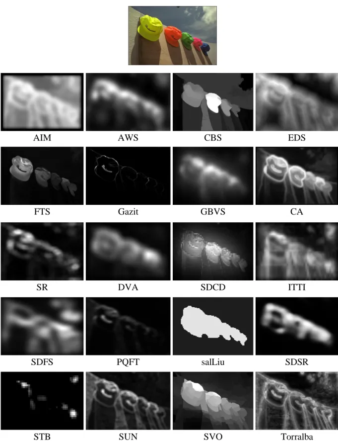
3.1 Illustration of saliency maps generated by twenty state-of-the-art saliency mod-els for one of the source images in the LIVE database . . . 33

3.2 Illustration of the rankings of saliency models in terms of CC, NSS and SAUC, respectively. The error bars indicate the 95% confidence interval . . . 37

(a) CC . . . 37

(b) NSS . . . 37

(c) SAUC . . . 37

3.3 Illustration of the rankings of IQMs in terms of the overall performance gain (expressed by∆PLCC, averaged over all distortion types, and over all saliency models where appropriate) between an IQM and its saliency-based version. The error bars indicate the 95% confidence interval . . . 44

3.4 Illustration of the comparison of the “information content map (ICM)” (c) ex-tracted from IWSSIM, VIF or IWPSNR, the “phase congruency map (PCM)” (d) extracted from FSIM and a representative saliency map(i.e., Torralba (b))for one of the source images in the LIVE database (a) . . . 45

3.5 Illustration of the rankings of the saliency models in terms of the overall per-formance gain (expressed by ∆PLCC, averaged over all distortion types, and over all IQMs where appropriate) between an IQM and its saliency based ver-sion. The error bars indicate the 95% confidence interval . . . 46

(20)

xx List of Figures

3.6 Illustration of the saliency maps as the output of the least profitable saliency

models and of the most profitable saliency models for IQMs. The original image

is taken from the LIVE database . . . 47

3.7 Illustration of the ranking in terms of the overall performance gain (expressed

by ∆PLCC, averaged over all IQMs, and over all saliency models where

ap-propriate) between an IQM and its saliency based version, when assessing WN, JP2K, JPEG, FF, and GBLUR. The error bars indicate the 95% confidence interval 48

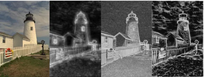
3.8 Illustration of an image distorted with white noise (WN) and its measured

nat-ural scene saliency and local distortions. (a) A WN distorted image extracted from LIVE database. (b) The saliency map (i.e., Torralba) based on the original image of (a) in the LIVE database. (c) The distortion_map of (a) calculated by

an IQM (i.e., SSIM) . . . 49

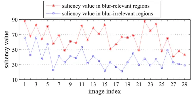
3.9 Illustration of the comparison of the averaged saliency residing in the

blur-relevant regions (i.e., positions of the strong edges based on the Sobel edge detection) and blur-irrelevant regions (i.e., positions of the rest of the image) for the 29 source images of the LIVE database. The vertical axis indicates the averaged saliency value (based on the saliency model called Torralba), and the horizontal axis indicates the twenty-nine test images (the content and ordering

of the images can be found in the LIVE database . . . 50

3.10 Illustration of a JPEG compressed image at a bit rate of 0.4b/p, and its

corres-ponding natural scene saliency as the output of a saliecny model (i.e., Torralba) 50

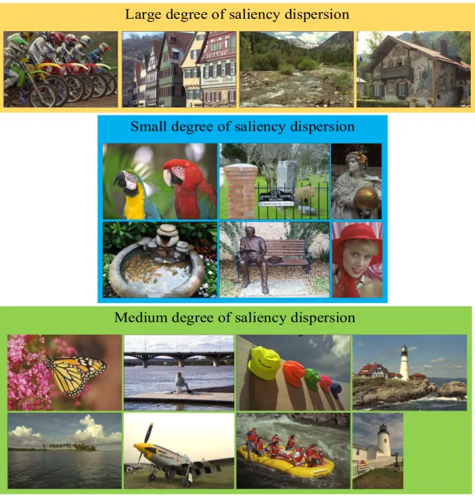
4.1 Illustration of reference images with different degrees of saliency dispersion

used in our experiment, which yield 288 test images . . . 56

4.2 Illustration of average DMOS of images assigned to a pre-defined level of

dis-tortion. The distortion levels are meant to reflect three perceptually distinguish-able levels of image quality (i.e., denoted as “High”, “Medium” and “Low”).

The error bars indicate a 95% confidence interval . . . 57

4.3 (a) Two sample stimuli of distinct perceived quality (DMOS = 95.96 (top image)

and DMOS = 32.26 (bottom image)). (b) The collection of human eye fixations over 20 subjects. (c) Grayscale fixation maps (the darker the regions are, the

lower the saliency is). (d) Saliency superimposed on the sample stimuli . . . . 59

4.4 Illustration of inter-observer agreement (IOA) value averaged over all stimuli

assigned for each subject group in our experiment. The error bars indicate a

(21)

List of Figures xxi

4.5 Illustration of inter-k-observer agreement (IOA-k) value averaged over all

stim-uli contained in our entire dataset. The error bars indicate a 95% confidence

interval . . . 61

4.6 The construction of stimuli in a single trail. The boxes indicate 35 stimuli in

random order. The 5 original images, as a group, are inserted in the front end,

middle and back end of each trail in random order . . . 63

4.7 Illustration of the impact of stimulus repetition on fixation behaviour. When

viewing 7 distorted versions of the same scene, the similarity in fixations (meas-ured by AUC) relative to its original decreases as the viewing order increases.

4.8 Illustration of the impact of stimulus repletion on fixation behaviour. When

viewing 3 times the same undistorted scene, the similarity in fixations (meas-ured by AUC) relative to its baseline taken from the TUD database decreases as

the viewing order increases. The error bars indicate a 95% confidence interval . 65

4.9 (a) Illustration of all distorted versions of a reference image (of a large degree

of saliency dispersion) and their corresponding fixation maps. The same layout of distorted images and fixation maps for a different reference image (of a small

degree of saliency dispersion) is illustrated in (b) . . . 66

4.10 Illustration of rankings of five distortion types contained in our database in terms of the SS-DSS similarity measured by CC, NSS and AUC, respectively. The

error bars indicate a 95% confidence interval . . . 68

4.11 The measured SS-DSS similarity in terms of CC, NSS and AUC for images of

different perceived quality. The error bars indicate a 95% confidence interval . 69

4.12 The measured SS-DSS similarity in terms of CC, NSS and AUC for images of different visual content (i.e., classified by the degree of saliency dispersion).

4.13 Comparison of performance gain between SS-based and DSS-based IQMs, with the effect of distortion type dependency. The error bars indicate a 95%

confid-ence interval . . . 74

4.14 Comparison of performance gain between SS-based and DSS-based IQMs with the effect of distortion level dependency. The error bars indicate a 95%

(22)

xxii List of Figures

4.15 Comparison of performance gain between SS-based and DSS-based IQMs with the effect of saliency dispersion degree dependency. The error bars indicate a

95% confidence interval . . . 75

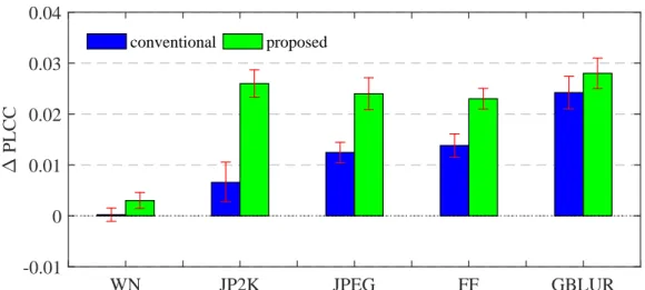
5.1 Comparison in performance gain using two combination strategies. The error

bars indicate the 95% confidence interval . . . 80

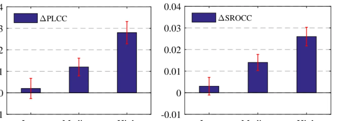
6.1 Performance gain (i.e., ∆PLCC and ∆SROCC) of saliency-augmented IQMs

for three degrees of IOA. Error bars indicate a 95% confidence interval . . . 87

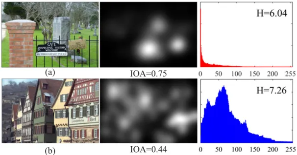
6.2 Natural scenes, their ground truth fixation maps, corresponding IOA scores, and

entropy of scene saliency. (a): an image with a few highly salient objects; IOA is high. (b): an image lacking salient objects; IOA is low. IOA values and fixation maps were determined from human eye fixations in the TUD eye-traking database 88

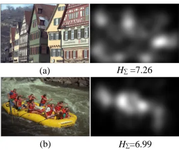
6.3 Illustration of two scenes with their corresponding ground truth saliency. (a)

an image with spread-out saliency. (b) an image with a large salient objects. Saliency maps were determined from human eye fixations in TUD eye-tracking

database . . . 89

6.4 Calculation of multi-level entropyHΣ. At each level the saliency map is

parti-tioned into blocks of equal size.HΣis found by adding the entropies computed

at each level of partition. Pmaxis the level with finest partitioning . . . 89

6.5 The absoulte value of the Pearson correlation (as shown for each data point)

between estimated saliency dispersion, HΣ, and its ground truth counterpart

IOA, for difference choices ofPmax. IOA values were determined for the same

set of images from three independent eye tracking databases . . . 90

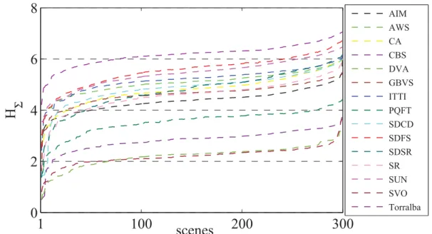
6.6 HΣcalculated for 300 scenes from the MIT300 database, using saliency values

generated by 15 state of the art saliency models. HΣ values are ordered from

lowest to highest for each model . . . 92

6.7 Comparison of performance gain (i.e., ∆PLCC) between saliency-augmented

IQMs using fixed and adaptive use of saliency for each saliency models . . . . 93

7.1 Illustration of the average DMOS of all stimuli for each perceived quality level

(23)

List of Figures xxiii

7.2 Illustration of the ground truth saliency maps for the original images used in our

database (a) and for samples of their distorted versions (b). The stimuli in the first row of (b) are placed in order of perceived quality (with the corresponding DMOS values listed at the bottom of (b)), and the third row of (b) shows the image patches extracted from the stimuli (i.e., as indicated by the red boxes in the stimuli) . . . 100

7.3 Illustration of the inter-observer agreement (IOA) averaged over all stimuli

as-signed to each group in our experiment. The error bars indicate a 95% confid-ence interval . . . 101

7.4 Illustration of the inter-k-observer agreement (IOA-k) averaged over all stimuli

contained in our entire dataset. The error bars indicate a 95% confidence interval 102

7.5 The measured SS-DSS deviation in terms of AUC, NSS and KLD for images

of different perceived quality (or distortion strength). The error bars indicate a 95% confidence interval . . . 103

7.6 Illustration of saliency maps generated by 17 state of the art saliency models for

one of the original images in CSIQ database and for one of its JPEG distorted versions . . . 105

7.7 Illustration of the rankings of saliency models in terms of predictive power

measured by SAUC. The error bars indicate a 95% confidence interval . . . 106

7.8 Illustration of the overall ability of saliency models in producing the correlation

(in terms of SROCC) between SS-DSS deviation and image quality . . . 109

7.9 Scatter plot of two variables: the saliency predictive power of a saliency model

(i.e., SAUC, based on the results of Fig. 7.7) and the quality predictive power of the corresponding SS-DSS model (i.e., SROCC, based on the results of Fig. 7.8) 110

8.1 Illustration of (a) a one-dimensional rectangular pulse signal and (b) its

recon-struction using phase spectrum . . . 115

8.2 Illustration of (a) a reference image and (b) its reconstruction using phase spectrum116

8.3 Illustration of (a) a distorted image and (b) its reconstruction using phase spectrum116

8.4 Illustration of the coarse-to-fine mechanism of the HVS. Note all lower scales

are upsampled to the original resolution o the image . . . 117

8.5 Illustration of (a) an original input and its corresponding (a) LD . . . 118

(24)

xxiv List of Figures

8.7 Example of the effect of the transmission error on chromatic channels . . . 119

8.8 Example of color saturation distortion. The distortion level increases from left

to right . . . 120

8.9 Illustration of the RG and BY channels for (a) an original image and (b) a

dis-torted image . . . 121 8.10 Plots of SROCC as a function of different parameters used in SDI for LIVE,

(25)

xxv

List of Tables

2.1 A comparison of five widely used image quality databases . . . 9

3.1 Performance gain (i.e., ∆PLCC) between a metric and its saliency-based

ver-sion over all distortion types for LIVE database. Each entry in the last row

represents the ∆PLCC averaged over all saliency models excluding the FM.

The standard deviations of the mean values range from 0.001 to 0.019 . . . 39

3.2 Performance gain (i.e.,∆SROCC) between a metric and its saliency-based

ver-sion over all distortion types for LIVE database. Each entry in the last row

represents the∆SROCC averaged over all saliency models excluding the FM.

The standard deviations of the mean values range from 0.002 to 0.017 . . . 40

3.3 Normality of the M-DMOS residuals. Each entry in the last column is a

code-word consisting of 21 digits. The position of the digit in the codecode-word represents the following saliency models (from left to right): FM, AIM, AWS, CBS, EDS, FTS, Gazit, GBVS, CA, SR, DVA, SDCD, ITTI, SDFS, PQFT, salLiu, SDSR, STB, SUN, SVO, and Torralba. “1” represents the normal distribution and “0”

represents the non-normal distribution . . . 41

3.4 Results of statistical significance testing based on M-DMOS residuals. Each

entry is a codeword consisting of 21 symbols refers to the significance test of an IQM versus its saliency based version. The position of the symbol in the codeword represents the following saliency models (from left to right): FM, AIM, AWS, CBS, EDS, FTS, Gazit, GBVS, CA, SR, DVA, SDCD, ITTI, SDFS, PQFT, salLiu, SDSR, STB, SUN, SVO, and Torralba. “1” (parametric test) and “*” (non-parametric test) means that the difference in performance is statistic-ally significant; “0” (parametric test) and “#” (non-parametric test) means that

(26)

xxvi List of Tables

3.5 Results of the ANOVA to evaluate the impact of the IQM, saliency model and

image distortion type on the added value of computational saliency in IQMs . . 43

4.1 Results of the ANOVA to evaluate the impact of distortion type, distortion level

and image content on the measured similarity between SS and DSS. df denotes

degree of freedom, F denotes F-ratio and Sig denotes the significance level . . . 68

4.2 Performance for 10 IQMs (PLCC without non-linear fitting) and their

corres-ponding saliency-based versions on our database with 270 distorted stimuli . . 73

4.3 Results of statistical significance testing for individual IQMs. “1” means that

the difference in performance is statistically significant with P<0.05 at the 95%

confidence level. “0” means that the difference is not significant . . . 73

5.1 Performance (in terms of PLCC, without nonlinear regression) of 12 IQMs and

their corresponding saliency-based versions (using either the conventional ap-proach or the proposed apap-proach) of the LIVE database. Note that PLCC is averaged over all saliency models and over all distortion types where appropriate 82

5.2 Performance (in terms of PLCC, without nonlinear regression) of 12 IQMs and

their corresponding saliency-based versions (using either the conventional

ap-proach or the proposed apap-proach) of the TID2013 and CSIQ database . . . 82

6.1 Performance for 10 IQMs (in terms of PLCC, without non-linear regression) on

all images of three databases, using versions which did not use saliency, always

used saliency, or adaptively used saliency according to saliency dispersion . . . 93

7.1 Configuration of test stimuli from LIVE image quality database . . . 97

7.2 The correlation between SS-DSS deviation and image quality, using KLD as the

similarity measure . . . 107

7.3 The correlation between SS-DSS deviation and image quality, using SDM as

the similarity measure . . . 108

7.4 The comparison of performance (in terms of SROCC) of two groups of models

in predicting image quality: one refers to the proposed SS-DSS model and one refers to state of the art image quality metrics . . . 109

8.1 Performance comparison of eight state of the art IQMs on three image quality

(27)

List of Tables xxvii

8.2 Overall rankings of IQMs based on SROCC . . . 123

8.3 Performance comparison in terms of SROCC for individual distortion types on

CSIQ dataset . . . 124

TID2013 dataset . . . 124

LIVE dataset . . . 125

(28)

(29)

1

Chapter 1

Introduction

1.1

Motivation

The past decades have witnessed a significant growth in using digital image stimuli as a means of information representation and communication. In current digital image processing and com-munication systems, image signals are subject to various distortions due to causes such as ac-quisition errors, lossy data compression, noisy transmission channels and limitations in image rendering devices. The ultimate image content received by the human visual system (HVS) dif-fers in image quality depending on the system and its underlying implementation. The undesired image quality degradation may affect the visual experiences of the end user or lead to interpreta-tion errors in visual inspecinterpreta-tion tasks [1]. Finding ways to effectively control and improve image quality has become a focal concern in both academia and industry [2]. Therefore, considerable efforts were made on appropriately tuning the parameters of image processing systems in order to enhance the image quality. While controlling the parameters of image processing systems is important for achieving high image quality, it is more crucial to evaluate image quality from the users’ perspective which is known as the subjective quality of experience (QoE) [3].

The subjective QoE can be directly measured by conducting subjective user study. Standardised subjective experimental methodologies have been proposed by the Radiocommunication Sector of the International Telecommunication Union (ITU-R) [4]. Though subjective test is regarded as the most accurate way of measuring QoE, it naturally has several disadvantages. First, the subjective test is expensive in terms of time and money. In addition, the results of the subject-ive QoE experiment collected in the laboratory environment may be inapplicable to the image quality assessment in real-world applications [3]. Moreover, the subjective test is impractical for any real-time applications.

To reduce the cost of subjective experiment and to facilitate the image quality assessment in real-world applications, image quality metrics (IQMs) — computational models for automatic assessment of perceived quality — have emerged as an important tool for the optimisation of modern imaging systems [5]. The performance of these IQMs is evaluated against the results

(30)

2 1.1 Motivation

of subjective test in order to check how well they can predict human scores. Nowadays, various IQMs are widely available in many imaging systems in a broad range of applications, e.g., for fine tuning image and video processing pipelines, evaluating image and video enhancement al-gorithms, and quality monitoring and control of displays. Substantial progress has been made on the development of IQMs over the last several decades, and many successful models have been devised. However, recent research shows that they demonstrate a lack of sophistication when it comes to dealing with real world complexity [6, 7, 8]. This makes image quality as-sessment a continued problem of interest. The fundamental challenge intrinsically lies in the fact that our knowledge about how the HVS assesses image quality and how to express that in an efficient mathematical model remains rather limited. Being able to reliably predict image quality as perceived by humans requires a better understanding of functional aspects of the HVS relevant to image quality perception, and optimal use of that to improve existing IQMs or devise more rigorous algorithms for IQMs.

Advanced IQMs benefit from embedding models of the HVS, such as contrast sensitivity func-tion [9] and visual masking [10]. Recently, a growing trend in image quality research is to investigate how visual attention — a mechanism that allows the HVS to effectively select the most relevant information in a visual scene — plays a role in judging image quality. More spe-cifically, the bottom-up stimulus-driven part of this attentional mechanism, i.e., visual saliency, is increasingly studied in relation to image quality. It is inferred that distortion in the salient areas is more annoying than that in the non-salient areas [11]. To understand whether this idea can be used to improve IQMs, initial effort has been made in the literature to investigate the added value of visual attention in IQMs by incorporating visual saliency models. Depending on the choice of saliency models and IQMs, some research findings revealed that the benefits of adding saliency to IQMs are marginal, whilst some research findings reported that saliency could significantly improve IQMs. Many saliency models and IQMs are available, the following issues such as how the benefits of inclusion of computational saliency in IQMs vary and what are the causes of this variation remain, which are worth further investigation.

Due to our limited understanding of the relation between visual attention and image quality, state of the art IQMs mainly focus on weighting local distortions (calculated by an IQM) with local saliency (resulted from a computational saliency model), yielding a more sophisticated means of image quality prediction. This concept, however, strongly relies on the simplification of the HVS that the visual attention aspects and the perception of local distortions are first treated separately and they are then combined artificially to determine the overall quality. The actual interactions between visual attention and image quality, however, are not considered. This simple combination of saliency and an IQM may downplay the importance of saliency in IQMs. It is highly desirable to investigate a perceptually optimised combination approach of adding saliency information to IQMs.

(31)

1.2 Hypotheses and Objectives 3

However, determining optimal use of visual attention aspects in IQMs is not straightforward [11]. The main challenge lies in the fact that how human attention affects image quality perception, and how to precisely simulate relevant functional aspects of the HVS in IQMs are not fully understood. To gain more knowledge of human vision, psychophysical studies have been un-dertaken to better understand visual attention aspects in relation to image quality assessment via eye-tracking [12, 13, 14, 15]. In general, these eye-tracking studies have shown that distortion occurring in an image alters gaze patterns relative to that of the image without distortion, and that the extent of the alteration tends to depend on several factors. These studies, unfortunately, are heavily limited by the choices made in their experimental design such as the use of a lim-ited stimulus variability [13], an insufficient number of subjects [12], and the involvement of massive stimulus repetition [14]. Therefore, the conclusions of these studies are either biased or hardly reveal statistically sound findings. To ensure the validity and generalisability of empirical evidence, it is desirable to investigate a more reliable methodology for collecting eye-tracking data for the purpose of image quality study.

In addition, a previous eye-tracking study [13] has shown that the deployment of fixations changes as a result of the appearance of visual distortions, and that the extent of the changes seems to be related to the strength of distortion. From this, it can be inferred that the changes of gaze patterns driven by distortion might be correlated with the variation in perceived qual-ity of natural images. Therefore, it is worth investigating the plausibilqual-ity of directly using the deviation of saliency as the proxy for image quality prediction.

1.2

Hypotheses and Objectives

This thesis is based on the following hypotheses:

• IQMs benefit from the addition of computational saliency, and the benefits of adding a

saliency term to an IQM can be further improved by taking into account the interactions between saliency and local distortions.

• Gaze is affected by distortion, and the deployment of fixations of a distorted image differs

from that of the original image without distortion. The deviation of fixation deployment can be used as a proxy for the prediction of image quality.

To validate the first hypothesis, following objectives are set in this thesis:

(32)

4 1.3 Contributions

• To investigate the interactions between visual saliency and image distortions via

eye-tracking.

• To improve saliency-based IQMs by taking into account the interactions between visual

saliency and local distortions.

To validate the second hypothesis, following objectives are set in this thesis:

• To investigate the relationship between the deviation of fixation patterns driven by

distor-tion and the perceived quality of natural images.

• To devise an IQM that is based on the measure of visual saliency deviation.

1.3

Contributions

This thesis presents the following contributions:

• We have conducted an exhaustive statistical evaluation to investigate the added value of

incorporating computational saliency in IQMs and how that depends on various factors. Knowledge as the outcome of this evaluation is highly beneficial for the image quality research community to have a better understanding of saliency inclusion in IQMs. The evaluation also provides useful guidance for saliency incorporation in terms of the effect of saliency model dependency, IQM dependency and image distortion type dependency.

• We have built a reliable eye-tracking database for image quality research. We

implemen-ted dedicaimplemen-ted control mechanisms in the experimental methodology to effectively elimin-ate potential bias due to the involvement of stimulus repetition. The resulting eye-tracking data provide insights into how visual attention behaviour is affected by visual distortions and how to optimise the inclusion of saliency in IQMs.

• We have proposed a new algorithm for the combination of saliency and IQMs by taking

into account the distraction power of local distortions. The proposed algorithm explicitly includes the interactions of visual saliency and distortion, outperforming the convention-ally used combination approach in terms of improving the performance of IQMs.

• We have proposed a new algorithm for reliably measuring the degree of saliency

disper-sion and used it to adaptively incorporate computational saliency in IQMs. We demon-strated that adaptive use of saliency according to saliency dispersion significantly outper-forms fixed use of saliency in improving the performance of IQMs.

(33)

1.4 Thesis Organization 5

• We have conducted a dedicated eye-tracking experiment to investigate the relationship

between the deviation of fixation patterns driven by distortion and the perceived quality of natural images. We demonstrated that the two variables mentioned above are highly correlated, which provides an empirical foundation for predicting image quality directly by the measurement of saliency deviation.

• We have devised a new IQM which is based on measuring saliency deviation between

a distorted image and its reference. Experimental results show that the proposed IQM is among the best performing IQMs while at relatively low computational cost in the literature.

1.4

Thesis Organization

• Chapter 2 introduces the background knowledge regarding to image quality assessment

and visual attention. The state of the art and challenges in the application of saliency information in image quality assessment are also presented.

• Chapter 3 details the statistical evaluation that investigates the capability of various

com-putational saliency in improving the performance of IQMs. The relationship between how well a saliency model can predict human fixations and to what extent an IQM can profit from adding this saliency model is also explored. This chapter also assesses de-pendencies of the performance gain that can be achieved by including saliency in IQMs. Practical issues regarding the application of saliency models in IQMs are discussed.

• Chapter 4 describes the conduct of a large-scale eye-tracking experiment which aims to

better understand visual saliency in relation to image quality assessment. A new exper-imental methodology is proposed and used in order to improve the reliability of eye-tracking data. Based on the resulting eye-eye-tracking data, the impact of image distortions on human fixations is assessed. This chapter also discusses the optimal use of saliency in IQMs.

• Chapter 5 follows up the research conducted in Chapter 4 and describes a new algorithm

that combines saliency and local distortions by taking into account the interactions between them.

• Chapter 6 investigates the content-dependent nature of the benefits of saliency inclusion

in IQMs and presents a saliency dispersion measure which can be used to adaptively incorporate saliency models in IQMs.

(34)

6 1.4 Thesis Organization

• Chapter 7 explores the relation between the deviation of fixation patterns driven by

dis-tortion and the perceived quality of natural images, via an eye-tracking experiment. This chapter also discusses the case of replacing eye-tracking data with computational saliency.

• Chapter 8 presents a new IQM that is based on measuring the deviations of visual saliency

features.

• Chapter 9 summarises the main conclusions of the thesis and discusses potential

(35)

7

Chapter 2

Background

2.1

Image Quality Assessment

Digital images usually undergo various phases of signal processing for the purpose of storage, transmission, rendering, printing or reproduction [1]. As a consequence, images are often sub-ject to distortions at every stage of the processing chain, resulting in various types of artifacts or transmission errors. To prevent the appearance of visual distortions and to optimise the digital imaging chain, modelling image quality is essential.

Traditionally, image quality is assessed subjectively by human observers. In the subjective im-age quality assessment, a number of human subjects are requested to rate the perceived quality of images in a carefully controlled environment. This methodology is considered as the most reliable way of assessing image quality, since human beings are the ultimate receivers of most visual information. However, subjective assessment is expensive, time-consuming and most im-portantly, unrealistic for practical applications. The increasing demand for digital visual media has pushed to the forefront the need for computational algorithms that can predict image quality as perceived by humans. These algorithms are referred to as objective image quality metrics (IQMs). In the past few decades, many IQMs have been proposed and they are now serving as an important tool in digital imaging systems to benchmark the performance of image processing algorithms off-line, to monitor image quality in real-time and to improve the design and testing phases of image processing products.

2.1.1

Subjective image quality assessment

Subjective image quality assessment is important as it provides ground truth on how human visual system (HVS) judges image quality. After quality scoring by human subjects, a single score — mean opinion score (MOS) — representing the perceived quality of an image is ob-tained by pooling the individual subjective ratings. Alternatively, the final score can also be interpreted as a differential mean opinion scores (DMOS), which represents the difference in

(36)

8 2.1 Image Quality Assessment

MOS between the distorted image and its corresponding reference. An image of higher per-ceived quality corresponds to a greater value of MOS or a smaller value of DMOS. Standardised methodologies for the subjective assessment of the quality of natural images do exist, such as the Radiocommunication Sector of International Telecommunication Union (ITU-R) BT.500-13 [4]. This document establishes methodologies including viewing conditions (e.g., viewing environment, monitor set-up and selection of test material), rating methods (e.g., experimental procedure), and raw data processing (e.g., outlier screening and data pooling).

Representative rating methods in (ITU-R) BT.500-13 contain Double Stimulus Continuous Scale (DSCQS) and Single Stimulus Continuous Quality Evaluation (SSCQE). In DSCQS, both the source stimulus and its distorted stimulus are shown to the observers for rating their quality. The difference between two ratings is used to represent the quality of the distorted stimulus. This method is often adopted to measure the quality of a visual signal processing system relat-ive to a pre-defined reference. In SSCQE, only the distorted stimuli are shown to the observers for quality rating as an attempt to reproduce the real-world viewing conditions where reference is normally unavailable. It should, however, be noted that each method documented so far con-tains advantages and disadvantages, and therefore, users should choose an appropriate method based on their own application environments. For example, double stimulus method is found to be more stable than single stimulus method for assessing small impairments due to that observ-ers are easier to detect the impairment in the presence of reference images. In contrast, single stimulus method is of practical relevance in the circumstance where no reference is available. In the meanwhile, research in image quality assessment has also lead to the emergence of vari-ous publicly available image quality databases. These databases can be used to benchmark the performance of IQMs. A typical image quality database usually contains a number of reference images, and for each reference there exist several distorted versions including various distortion types and distortion levels. The database also gives a MOS/DMOS for each stimulus. There are about twenty image quality databases in the literature, among which LIVE [16], CSIQ [17], TID2013 [18], IVC [19] and MICT [20] are the most widely used databases. The reliability of the above-mentioned databases is widely recognised in the image quality community since they were collected using standardised methodologies in controlled experimental environment [21]. In this thesis, we also use these five image quality databases for assessing the performance of IQMs to ensure an unbiased performance evaluation. Moreover, these databases are among the largest image quality databases in the literature in terms of stimulus variability especially for TID2013, CSIQ and LIVE. Additionally, as most of the IQMs are benchmarked on these databases, a direct comparison between the proposed IQMs in this thesis and other IQMs in the literature can be made immediately if we also use these databases. A detailed comparative study of some well-established databases was conducted in [21] regarding e.g., the composi-tion of stimuli, experimental design and subjective rating. We summarize the details of these

(37)

2.1 Image Quality Assessment 9

Table 2.1: A comparison of five widely used image quality databases.

No. of ref. images No. of dist. images No. of dis. types No. of subjects

LIVE 29 799 5 29

TID2013 25 3000 24 971

CSIQ 30 866 6 35

IVC 10 185 5 15

MICT 14 168 2 27

databases as below and list their main features in Table. 2.1.

The LIVE database consists of 779 images distorted with five distortion types, i.e., JPEG com-pression (i.e., JPEG), JPEG2000 comcom-pression (i.e., JP2K), white noise (i.e., WN), Gaussian blur (i.e., GBLUR) and simulated fast-fading Rayleigh occurring in (wireless) channels (i.e., FF). Per image the database also gives a differential mean opinion score (DMOS) with a scale

of zero to one hundred. The resolution of the images ranges from 634 × 438 to 768 × 512

pixels. The subjective ratings were obtained from 29 participants.

The TID2013 database is currently the largest database in the literature. It consists of 3000 distorted images derived from 25 reference images. There are 24 distortion types in the data-base, namely additive Gaussian noise (AGN), additive noise in color components (ANC), spa-tially correlated noise (SCN), masked noise (MN), high frequency noise (HFN), impulse noise (IN), quantization noise (QN), Gaussian blur (GB), image denoising (DEN), JPEG compres-sion (JPEG), JPEG2000 comprescompres-sion (JP2K), JPEG transmiscompres-sion errors (JGTE), JPEG2000 transmission errors (J2TE), non eccentricity pattern noise (NEPN), local block-wise distortions (Block), mean shift (MS), contrast change (CTC), change of color saturation (CCS), multiplic-ative Gaussian noise (MGN), comfort noise (CN), lossy compression of noisy images (LCNI), image color quantization with dither (ICQD), chromatic aberrations (CHA) and sparse sampling and reconstruction (SSR). Per reference image, there are five distorted versions for each

distor-tion type. All the stimuli in the TID2013 database are at a resoludistor-tion of 512 × 384. The

subjective ratings were obtained from 971 participants.

The CSIQ database consists of 866 distorted images derived from 30 reference images with

each at a resolution of 512×512. It contains 5 distortion types, namely additive Gaussian white

noise (AGWN), JPEG compression (JPEG), JPEG2000 compression (JP2K), additive Gaussian pink noise (AGPN), Gaussian blurring (GB) and global contrast decrements (GCD). The rating scores were obtained from 35 participants.

The IVC database consists of 185 distorted images derived from 10 reference images with each

(38)

blur, 50 images distorted with JPEG compression, 25 images distorted with JPEG compression of the luminance channel only, 50 images distorted with JPEG2000 compression and 40 images distorted with locally adaptive-resolution coding. The subjective ratings were obtained from 15 participants.

The MICT database consists of 168 distorted images derived from 14 reference images with

each at a resolution of 768×512. It contains two distortion types: JPEG compression artifacts

and JPEG2000 compression artifacts with each corresponding to 84 distorted images. The rating scores were obtained from 27 participants.

2.1.2

Objective image quality assessment

In the field of signal processing, signal fidelity metrics, e.g. mean square error (MSE) and peak signal-to-noise ratio (PSNR) are commonly used to objectively assess the signal quality. They remain widely used due to their simplicity and generalizability for implementation. However, these metrics usually show unsatisfactory performance when handling visual signals such as images and videos, and they have been long criticized for their inconsistency with how humans judge image quality [22]. The main reason account for this poor correlation between the ob-jective measurements and human judgements is that these signal fidelity metrics are based on several implicit assumptions which may not be true for visual signals. For example, PSNR assumes that the image signals and distortions are independent, and the perceptual quality is purely determined by distortions independent of image content. Another assumption is that the perceived quality is independent of the spatial locations of distortion.

To improve the performance of objective image quality assessment, a lot of effort has been made on designing IQMs that take into account the way humans perceive image quality. The IQMs available in the literature differ in their application, ranging from metrics that assess a specific type of visual distortion to those that evaluate the overall image quality. These IQMs can be generally classified into two categories, namely the perception-driven metrics and the signal-driven metrics. The former attempts to simulate relevant functional components of the HVS, while the latter focuses on visual signal analysis.

The goal of the perception-driven IQMs is to come close to the behaviour of the HVS. Advances in human vision research have increased our understanding of the mechanisms in the HVS, and thus allowed integrating these psychophysical findings in designing IQMs [23, 24, 25]. Some well-established models that address the low-level aspects of early vision, such as contrast sensitivity [9], visual masking [10], luminance adaptation [26] and foveated vision [5] have been implemented in IQMs. Popular IQMs include Visual Signal-to-Noise Ratio (VSNR) [27],

(39)

2.1 Image Quality Assessment 11

Most Apparent Distortion (MAD) [28] and the Noise Quality Measure (NQM) [29]. We hereby briefly introduce these IQMs as below:

• VSNR is inspired by the psychophysical experiments related to the detectability of

dis-tortions. A contrast threshold is modelled to determine the visibility of distortions in natural images. If the distortions are below the threshold, the quality of the distorted im-age is considered to be perfect. If the distortions are detectable by the HVS, the strength of distortions is quantified by the Euclidean distance between two image features of the reference and distorted images.

• MAD measures the image quality with two separate strategies based on the characteristics

of the HVS. For images with high quality, MAD mimics how the HVS perceives visual artifacts in the presence of the image content whereas for images with low quality, MAD simulates how the HVS recognises image content in the presence of distortions.

• NQM is inspired by the psychophysical findings that frequency distortions and additive

noise have independent effects on the visual quality perception. Thus, NQM decouples all distortions into these two forms and quantifies their impact on the HVS separately. Then, the final quality prediction is computed by integrating the two measures.

These HVS-based IQMs have been proven more reliable than the traditional signal fidelity met-rics. Nevertheless, the perception-driven modelling approach remains limited in its sophistica-tion and thus in its performance, mainly due to the fact that our knowledge of the HVS is limited and that it is impossible to precisely simulate all perception-related aspects in the HVS.

Instead of imitating the functional operations of the HVS, the signal-driven approach treats the HVS as a black box. This approach is usually concerned with the overall functionality of the HVS, and concentrates on image statistics as well as analysis of distortions. Many IQMs based on this philosophy have been devised and demonstrated rather effective in predicting image quality. Representative IQMs in this category include the universal quality index (UQI) [30], the structural similarity index (SSIM) [31], the multi-scale SSIM (MS-SSIM) [32], the in-formation content weighting PSNR (IWPSNR) [33], the inin-formation content weighting SSIM (IWSSIM) [33], the visual information fidelity (VIF) [34], and the feature similarity index [35], the generalized block-edge impairment metric (GBIM) [36], the no-reference perceptual blur metric (NPBM) [37], the just noticeable blur metric [38], and the no-reference blocking artifact measure [39]. We hereby briefly introduce these IQMs as below:

• UQI measures the image quality degradation as a combination of the loss of pixel

(40)

• SSIM is based on the observation that the HVS is highly adapted to extract structural

information from a visual scene. Thus, SSIM attempts to measure image quality by quan-tifying the structural similarity between a distorted image and its original version.

• MS-SSIM represents a refined and flexible version of the single-scale SSIM,

incorporat-ing the variations of viewincorporat-ing conditions.

• Based on the hypothesis that the importance of the locally measured distortion is

propor-tional to the local information content, IWPSNR was proposed by extending PSNR with an extra weighting process to refine the relative importance of local distortions.

• Similarly, IWSSIM was also devised by refining the local distortion measured by SSIM.

• VIF aims to assess image quality using natural scene statistics. The shared information

between an original image and its distorted version is used to measure the quality of the distorted image.

• Based on the assumption that phase congruency and gradient magnitude play

comple-mentary roles in characterising local image quality, FSIM predicts image quality by meas-uring the deviations of these two features between an original image and its distorted version.

• GBIM measures the quality of images that are distorted with blocking artifacts as an

inter-pixel difference across block boundaries.

• NBAM considers the visibility of the blocking artifacts by computing the local contrast

in gradient.

• NPBM measures the quality of blurring images based on extracting sharp edges in an

image and measuring the width of these edges.

• JNBM refines the measurement of the spread of the edges by integrating the concept of

just noticeable blur.

In general, compared to the perception-driven IQMs, signal-driven IQMs provide simplified solutions which can be easily embedded in real-time applications. Additionally, signal-driven IQMs do not rely on the success of modelling the rather complex HVS. However, it should be noted that the effectiveness of the signal-driven IQMs depends on the relevance of prior knowledge of image statistics.

It should be noted that there have been a variety of IQMs that are based on machine learning techniques. They have become an emerging category of IQM apart from the signal-driven IQMs

(41)

2.1 Image Quality Assessment 13 Feature extraction Distortion channel Ancillary channel RR IQM Quality score Original image Side inforamtion Distorted image Original image Distorted image FR IQM Quality score

Distorted image NR IQM Quality _score

(a) general framework of full-reference IQMs

(b) general framework of no-reference IQMs

(c) general framework of reduced-reference IQMs

Figure 2.1: General frameworks of full-reference (FR), reduced-reference (RR) and no-reference (NR) metrics.

and perceptual-driven IQMs. Generally, these learning-based IQMs extract features from image first, and then use machine learning methods to map the image features to a single quality score. These learning-based IQMs are not considered in this thesis. How to effectively apply visual saliency as an image feature in learning-based IQMs is worth investigating and may be considered in future work.

IQMs can also be classified into full-reference (FR), reduced-reference (RR) and no-reference (NR) metrics, depending on to what extent the quality assessment algorithms rely on the un-distorted reference. Figure 2.1 illustrates the general frameworks for IQMs in each category. FR metrics require the full access to the reference and are generally implemented using the framework as shown in Fig. 2.1(a). They assume that the undistorted reference image exists and is fully available. These IQMs are also called image similarity or fidelity measurement since the quality scores predicted by these IQMs are based on quantifying the similarity or differ-ence between the referdiffer-ence image and the distorted image. In contrast, NR metrics attempt to

(42)

14 2.2 Visual Saliency

predict the perceived quality solely based on the distorted image. The general framework of the IQMs in this category is illustrated in Fig. 2.1(b). NR metrics can be further classified into general-purpose NR IQMs and distortion-specific NR IQMs. General-purpose NR metrics aim to measure the quality of images without any information from the distortion. Most of these metrics are based on feature extraction and training on subjective quality scores. On the other hand, distortion-specific NR metrics focus on a specific type of distortion, e.g., JPEG/JPEG2000 compression artifacts, ringing or blurring, and characteristics of specific distortions are utilized to increase the performance of NR IQMs. In the scenarios where the reference is partially avail-able (e.g., in complex communication networks), RR metrics are meant to assess image quality with partial information extracted from the reference (e.g., some image features). Figure 2.1(c) shows the processing pipeline for RR image quality assessment systems. At the sender’s side, some image features are extracted from the original undistorted images. These extracted fea-tures are then transmitted to the receiver’s side through an ancillary channel as side information. This information is later used to assist the quality assessment of the image transmitted through the distorted channel. Generally, FR metrics achieve higher performance than RR and NR met-rics due to the availability of extra information extracted from reference images [40]. However, the requirement for the access of reference images may limit the deployment of FR metrics in certain applications.

It is worth noting that the IQA framework can be easily extended to a video quality assessment (VQA) framework since one straightforward design of video quality metrics (VQMs) may be applying current IQMs on a frame-by-frame basis. The overall video quality can then be derived by pooling the frame level quality scores with other video features [41]. Therefore, designing IQMs of high performance is of fundamental importance to the visual quality research com-munity.

2.2

Visual Saliency

It is estimated that the visual data travelling into our eyes are approximately 108 _to ₁₀9 _bits

per second [42]. Dealing with this data flow in real-time is an incredibly heavy mission for the HVS. Fortunately, only a portion of the data is selected and processed further in detail by

the HVS. This selective mechanism in the HVS is called visual attention. Such an attentional

behaviour is believed to be guided by two types of mechanisms, namely the stimulus-driven, up mechanism and the expectation-driven, top-down mechanism [43]. The bottom-up attention is mainly driven by the attributes of visual scenes including orientation, contrast, colour, motion and etc. The top-down attention is associated with cognitive aspects including experience, memory and cultural background and etc. In the area of computer vision, visual

(43)

2.2 Visual Saliency 15

attention is mainly concerned with the former attentional mechanism due to its simplicity, which

is often interchangeably referred to asvisual saliency[44].

2.2.1

Eye-Tracking

The most straightforward way to study human visual attention is through the use of eye-tracking [45, 46, 47]. In an eye-tracking experiment, the eye movements of observers are recorded when viewing images. Neuroscientists, psychologists and computer vision engineers are using eye-tracking in a broad range of applications including medicine [48], engineering [49], psycho-logy [50], education [51], robotics [52], marketing [53] and gaming [54].

The devices to obtain the eye-tracking data are called eye-trackers. They can be generally classified into three categories, namely the optical tracking system, the eye attached tracking system and the electrooculography (EoG) tracking system. The optical tracking is the most commonly used method which captures the infrared light reflected from the eye. In eye attached tracking systems, eye movements are recorded by measuring the movements of an attachment (e.g., contact lenses with a magnetic sensor embedded in) to human eyes. In EoG tracking systems, eye movements are measured by quantifying the change of electric signals around human eyes. Among these tracking systems, EOG tracking systems are less accurate due to noise in the electric signal. Eye attached systems suffer from potential slips of the attachment. Therefore, the optical tracking method is the most widely used approach in the literature. The eye-tracker used in this thesis (i.e., SensoMotoric Instrument (SMI) RED-m) belongs to the optical tracking category. Moreover, it features a contact-free property that allows free head movement. Therefore, it enables a collection of eye-tracking data over long duration without causing discomfort to subjects.

Abundant information is contained in the eye-tracking data, including fixations, saccades, pupil dilation and scanpaths [55]. Among these variables, researchers in the field of computer vision are concerned with fixation as they provide important information for bottom-up saliency. Eye fixation is defined as a spatially stable gaze lasting for several hundreds of milliseconds [56]. Afixation map, also known asgaze mapof an image is often derived by accumulating all fixa-tions of all observers recorded for that image. The reason to combine fixafixa-tions from all observ-ers instead of using an individual’s fixations is to minimise the bias due to pobserv-ersonal preference. A fixation map can be simply visualised as a binary map with “1” representing fixated locations and “0” representing unfixated locations or further post-processed into a grayscale map which is constructed by convolving a Gaussian kernel with each of the fixations. The binary map gives exact pixel locations of fixations in an image, while the grayscale map reflects attentive regions of the visual field. Both types of fixation maps are being used in different applications.

(44)

A number of eye-tracking databases have been created for computer vision researchers to better understand visual attention behaviour and to benchmark saliency prediction algorithms [57]. Unfortunately, standardised methodologies for eye-tracking data collection do not exist. Eye-tracking experiments are usually conducted in different laboratories and under different con-ditions and the raw data are processed in slightly different ways. Therefore, the usefulness of these databases may differ for different applications.

2.2.2

Visual saliency models

Computational models of visual saliency (i.e., bottom-up aspects of visual attention) aim to pre-dict where people look in images. Note top-down aspects of visual attention are complex and are therefore rarely included in a saliency model. So far, many saliency models have been pro-posed in the literature and they have proven useful to various applications, including computer vision (e.g., object detection [58] and object recognition [59]), robotics (e.g., human-machine interaction [60]) and visual signal processing (e.g., region-of-interest-based compression [61] and image resizing [62]).

Pioneering work in saliency modelling was conducted in 1980s when Tresiman and Gelade

proposed theFeature-Integration Theory (FIT)[63].The FIT states that when the HVS perceives

a visual stimulus, different categories of image features are first parallelly selected and then combined in a later stage in order to identify objects. Following this framework, Koch and

Ullman [43] proposed a mathematical descriptor for the FIT, resulting in a so-called saliency

mapthat represents conspicuousness of a visual scene. This mathematical descriptor was further

implemented by Itti et.al [64] for the construction of a saliency model, which has become one of the best-known models in the literature. Nowadays, a large number of saliency models are available in the literature, among which a majority of them are based on the FIT framework. In general, these saliency models take a three-step approach. First, multi-scale image pyramids of the input image are created, mimicking the multi-channel and multi-scale nature of the HVS [6]. In the second step, various image features are extracted from the pyramids, resulting in a set of feature maps. Finally, these feature maps are normalized and combined to form the final saliency map.

Saliency models can be categorized into pixel-based models and object-based models. The pixel-based models aim to highlight pixel locations where fixations are likely to occur. The object-based models focus on detecting salient objects in a visual scene. The majority of sa-liency models in the literature are pixel-based sasa-liency models, such as ITTI [64], STB [65], AIM [66], SUN [67], CovSal [68] DVA [69], GBVS [70], Torralba [71], SR [72], PQFT [73], EDS [74], AWS [75], Gazit [76], SDSR [77], SDSF [78] and SDCD [79]. Representative

(45)

2.2 Visual Saliency 17

object-based saliency models include CBS [80], FTS [81], salLiu [82], SVO [83] and CA [84]. In general, there are less object-based saliency models in the literature if compared with the number of pixel-based models. One of the reasons may be that the object segmentation pro-cess involved in a typical object-based model remains as an issue of computer vision. All the saliency models mentioned above are used in this thesis and are briefly summarized as below:

• ITTI is perhaps the first notable work in the field of computational saliency modelling,

which combines multiscale image features into a single topographical saliency map.

• STB is meant to improve the output of ITTI for extracting the region of interest (ROI) —

a binary mask that highlights the portion of an image where observers pay their attention to.

• AIM computes visual saliency using Shannon’s self-information measure of visual

fea-tures.

• SUN compares the features observed at each pixel location to the statistics of natural

images and calculate the probability of each pixel to be salient using Bayes’ rule.

• CovSal employs a local definition of saliency and measures the saliency of a pixel as how

much it differs from its surroundings.

• DVA measures saliency with an attempt to maximize the entropy of the sampled visual

features.

• GBVS is based on graph theory and is achieved by concentrating mass on activation maps,

which are formed from certain raw features.

• Torralba measures saliency by incorporating several low-level features including contrast,

colour, edge and orientation and two high-level features including objectness and context.

• SR is a simple model based on Fourier transform, where both the amplitude spectrum and

phase spectrum are obtained.

• PQFT combines the phase spectrum information and the motion information to form a

spatiotemporal saliency models.

• EDS relies on multi-scale edge detection and produces a simple and non-parametric

method for detecting salient regions.

• AWS computes saliency by taking into account the decorrelation and distinctiveness of

(46)

• Gazit employs a local-regional multi-level approach to detect edges of salient objects.

• SDSR computes the saliency using local descriptors from a given image which measure

likeness of a pixel to its surroundings.

• SDFS measures saliency by combining global image features from frequency domain and

local image features from spatial domain.

• SDCD works in the compressed domain and adopts intensity, colour and texture features

for saliency detection.

• salLiu focuses on the salient object detection problem for images, using a conditional

random field to learn ROI from a set of pre-defined features.

• CA employs multiple principles: local low-level features, visual organisation, global

fea-tures and high-level feafea-tures to separate the salient object from the background.

• FTS aims for the detection of well-defined boundaries of salient objects, which is achieved

by retaining more frequency content from the image.

• CBS is formalized as an iterative energy minimization framework, which results in a

binary segmentation of the salient object.

• SVO detects salient objects by fusing the cognitive-based objectness together with the

image-based saliency.

Alternatively, saliency models can also be classified into spatial models and spatiotemporal models. Spatial models predict visual saliency according to the spatial cues only whereas spa-tiotemporal models estimate saliency based on both the spatial and temporal features of video sequences. Most saliency models in the literature fall into the former category, since simulating the effect of temporal saliency cues on the fixation deployment