www.geosci-model-dev.net/3/669/2010/ doi:10.5194/gmd-3-669-2010
© Author(s) 2010. CC Attribution 3.0 License.
Geoscientific
Model Development
Physically-based data assimilation
G. Levy1, M. Coon1,†, G. Nguyen2,*, and D. Sulsky2 1NorthWest Research Associates, Seattle, Washington, USA
2Department of Mathematics and Statistics, University of New Mexico, Albuquerque, New Mexico, USA
*currently at: The School of Civil Engineering, University of Sydney, Sydney, NSW, Australia †deceased
This paper is dedicated to our friend and colleague, Max Coon. He initiated, inspired and guided our work on sea ice. We will miss him.
Received: 6 April 2010 – Published in Geosci. Model Dev. Discuss.: 11 May 2010
Revised: 10 November 2010 – Accepted: 19 November 2010 – Published: 29 November 2010
Abstract. Ideally, a validation and assimilation scheme should maintain the physical principles embodied in the model and be able to evaluate and assimilate lower dimen-sional features (e.g., discontinuities) contained within a bulk simulation, even when these features are not directly ob-served or represented by model variables. We present such a scheme and suggest its potential to resolve or alleviate some outstanding problems that stem from making and applying required, yet often non-physical, assumptions and proce-dures in common operational data assimilation. As proof of concept, we use a sea-ice model with remotely sensed obser-vations of leads in a one-step assimilation cycle. Using the new scheme in a sixteen day simulation experiment intro-duces model skill (against persistence) several days earlier than in the control run, improves the overall model skill and delays its drop off at later stages of the simulation. The po-tential and requirements to extend this scheme to different applications, and to both empirical and statistical multivari-ate and full cycle data assimilation schemes, are discussed.
1 Introduction
Data assimilation deals with the optimal combination of ob-servations and a model forecast, or background field, into an analysis field that forms the basis for the next forecast (Daley, 1992). Originating in meteorology, data assimilation is now
Correspondence to: G. Levy
used extensively with all operational geophysical models to improve model predictions and performance based on avail-able observations. Most modern data assimilation techniques fall into two main categories: empirical methods, and meth-ods based on statistical estimation theory (Talagard, 1997). Empirical methods, like dynamic relaxation (a.k.a. nudging, Hoke and Anthes, 1976) are most useful with new data and data sets for which error estimates and/or the error covari-ance structure are not known or available, as is the case for our application. Although implemented differently, it can be shown that all assimilation methods based on statistical esti-mation theory (hereafter, statistical data assimilation) can be regarded as an extension of optimal interpolation (OI) and are mathematically based on optimization algorithms, most com-monly the least square minimization principle. The equiva-lency of statistical data assimilation methods, including OI, Bayesian data assimilation, Kalman Filtering (KF) and vari-ational techniques, is shown, for example, in Kalnay (2003). Current and future data assimilation systems must cope with some known issues that stem from constraints, limitations, and errors in both the models and the observations assimi-lated, namely:
i. During initialization, if the analyzed field, based on the data, does not match a realizable model state, noise is generated when the model integrates forward in time and this noise can severely impair forecast skill, and may lead to “the rejection problem” (Daley, 1992). ii. Assimilation systems do not have a simple, quantitative
directly defined by either observations or model vari-ables. Assimilation methods that ignore these features often force observed data onto models in a non-physical way. Such features occur frequently in geophysical ap-plications and are associated with discontinuities and other important physical and dynamical processes on multiple scales.
iii. The observed data that are assimilated do not match the variables predicted by the model, requiring param-eterizations that are not consistent with the data or the physics.
These issues arise when the validation and assimilation schemes do not maintain the physical principles embodied in the model and are unable to evaluate and assimilate lower di-mensional features (e.g., discontinuities) contained within a bulk simulation that are not directly observed or represented by model variables. Under these circumstances, assimila-tion can lead to the violaassimila-tion of physical principles and the loss of information contained in the lower dimensional fea-tures. Conversely, models that resolve such features and the associated physics well, yet imprecisely, are often penalized by traditional schemes, leading to (perceived or real) poor model performance and forecasting skill scores. This loss of information can become deleterious in model improvements when observations are sparse, fuzzy, or irregular.
The aforementioned issues have been reported in different applications of data assimilation. For example, in an assim-ilation experiment with a sea-ice model, Lindsay and Zhang (2006) illustrate that some fields in the model no longer strictly adhere to the physical principles of the model when data assimilation is accomplished through nudging (dynamic relaxation). They also note that similar inconsistencies arise when variables that originate from independent datasets are assimilated independently. Dai et al. (2006), in another sea-ice model simulation using optimal interpolation, show that the assimilated data degrade the solution at later stages be-cause the underlying physical assumptions in the model are compromised. An ensemble Kalman filter (EnKF) assimila-tion in a wildfire model by Mandel et al. (2008) resulted in nonphysical states especially far away from the data. When discontinuous processes are modeled the problems of initial-ization can be exacerbated as shown by Vukicevic and Bao (1998) in a meteorological variational (4DVAR) data assim-ilation system. In that study, the linearization errors asso-ciated with discontinuous convective parameterizations were non-negligible and affected the assimilation results both lo-cally and globally.
This paper considers a new paradigm for assessing model performance and for comparing model results with observa-tional data. The resultant assimilation and validation scheme is compatible with state of the science methods and is capable of handling lower dimensional features in a bulk simulation. This scheme addresses issues (i), (ii), and (iii) above. The underlying principle for our assimilation algorithm is to use
data to precondition model variables or material properties that allow internal model physics to generate future model states that agree better with observed data. The new scheme is tested with a sea ice model (Schreyer et al., 2006; de-scribed in Sect. 2.3 and Appendix A) and RADARSAT Geo-physical Processor System (RGPS; Kwok, 1998) data, in a physically-based nudging context for one assimilation cycle. We employ a fuzzy verification metric of Levy et al. (2008) and standard skill scores of Murphy (1988) to evaluate model performance. We show that implementing the new assimila-tion scheme introduces model skill (against persistence) sev-eral days earlier than in the control run, improves the over-all model skill, and delays its drop off at later stages of the simulation. We conclude with some thoughts about extend-ing this method to a full assimilation cycle and to statistical-estimation data assimilation systems.
2 Physically-based assimilation and validation
2.1 Data assimilation algorithm
Standard practice in data assimilation is to subtract model estimates of state variables interpolated to observation loca-tions, from observed values (the background field), to pro-duce innovations (or observation increments). Objective analysis of these innovations onto the model grid is then used for initialization of the model. The algorithm for validation and assimilation proposed and tested here assumes an ade-quate measure for model validation and verification exists, even for lower dimensional features. In it, feature extraction and assessment (see Sects. 2.2 and 2.4) take the place of ob-jective analysis for lower dimensional features. We use the fuzzy verification metric, RI, of Levy et al. (2008), Eq. (B1), as a benchmark for assessment.
2.2 Lower-dimensional features in sea ice observational data
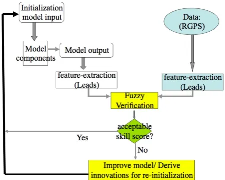
We choose to test the new assimilation scheme in a sea-ice environment where lower dimensional features in the form of Linear Kinematic Features (LKFs; Kwok, 2001) are abun-dant and observable. LKFs represent discontinuities in the sea ice (e.g., leads or ridges, Coon et al., 2007). Although not directly measured or resolved by observing systems or most models, LKFs can be related to model resolvable phys-ical or material properties. LKFs persist sufficiently to allow simplified testing of our scheme that adjusts model variables at initialization. A general assimilation scheme would call for the model state to be updated regularly based on the data and their agreement with the model output, rather than just initially. The adjustments can be implemented at set inter-vals (i.e., in a continuous data assimilation), or only when agreement or skill score falls below a certain threshold. This validation and assimilation technique is schematically de-picted in Fig. 1 for both the general case and the ice model implementation tested. The data we use come from the RADARSAT Geophysical Processor System (RGPS), which was developed by the Polar Remote Sensing Group at the Jet Propulsion Laboratory (JPL) to extract sea ice motion data from SAR imagery (Kwok et al., 1990). At an initial time, a set of points forming a regular grid is located in the SAR data sets. Then, in the images resulting from subsequent satel-lite passes (approximately every 3-days), the original points are found again using area-based and feature-based tracking. This procedure provides displacements for each point. If the set of points in the original configuration is viewed as the vertices of square cells, then the motion of the points deter-mines the deformation of the cells. With this interpretation, grid quantities such as the divergence, shear, and vorticity, can be calculated using the nodal displacements.
The RGPS deformation products are based on the assump-tion that the displacements and velocities are smooth func-tions of the spatial coordinates. However, if the dominant form of deformation of multiyear ice is in the opening, clos-ing, and shearing of linear features or leads, then the dis-placements and velocities can be discontinuous. In Coon et al. (2007) we discuss the kinematics associated with strong discontinuities that describe possible jumps in displacement or velocity. Specifically, we determine a jump in displace-ment and the orientation of this jump that account best for the observed deformation of an RGPS cell. We use this treatment of the data for feature extraction and subsequent assimilation of the information.
2.3 Sea-ice model and simulations
The sea-ice simulations we perform to demonstrate our scheme use an elastic-decohesive constitutive model for the sea ice (Schreyer et al., 2006). The model was developed for predicting the initiation and opening of leads in the Arctic
Fig. 1. Schematic of the validation and assimilation algorithm
illus-trated for the general case and (in parentheses) lower dimensional features and the sea ice model and data tested. The implementa-tion and testing on lower dimensional features involve the assimila-tion of RGPS data processed to show regions of high deformaassimila-tion. The model state may be updated by changing material properties based on agreement of lower dimensional features and fuzzy met-rics scores. For example, if the data indicates the presence/absence of LKFs in a region, a jump in displacement is determined to ac-count for the observed RGPS deformation of the cell.
ice. Once the existence of leads is taken into account, the remaining motion of the ice has small deformations and is appropriately described as elastic. Several features were de-signed into the model. First, the model was constructed to transition from observed brittle failure under tension, to compressive brittle failure under moderate compression, and to a plastic-like faulting under large confinement (Schulson, 2004). The various modes of failure occur in the model, de-pending on the stress state in the material. Where the tran-sitions occur in stress space depends on the material param-eters and can be adjusted based on empirical data. Second, the model can handle multiple cracks at a point, and there-fore can predict crack branching. Third, the numerical imple-mentation of the model is accomplished similarly to standard plasticity models. Thus, in principle, modular codes that call a subroutine to implement the constitutive model can substi-tute the elastic-decohesion model if it proves worthwhile. A final aspect of the model is the ability to build in pre-existing planes of weakness that may be due to pre-existing, partially frozen leads, for example. It is this feature that we exploit in order to initialize simulations using observed data. More information about this model can be found in Appendix A.
hour wind fields from NCEP reanalysis are used to determine the wind drag and the ocean currents are updated daily using output from an ocean model (MITgcm, Marshall et al., 1997) run independently from the ice simulation.
The momentum equation is solved using the material-point method (Sulsky et al., 2007). With the material-material-point method (MPM), a set of material points is identified in the body of fluid or solid that is tracked throughout the defor-mation process. Each material point has a mass, position, velocity and stress, as well as material parameters and inter-nal variables as needed for constitutive models or thermo-dynamics. These material points provide a Lagrangian de-scription of the material that is not subject to mesh tangling because no connectivity is assumed between the points. This Lagrangian frame naturally models convection and transport since the trajectory and history of each material point is fol-lowed. Each point carries material properties without error, and history variables can be integrated along the trajectory. However, computing gradients for solution of the momen-tum equation is complicated in this representation since the neighbors of a given point are not known a priori, and can change during a simulation. To keep the computational work linear in the number of material points, a second discretiza-tion is used for solving the momentum equadiscretiza-tions. This repre-sentation of the solution is often a regular, background mesh that covers the computational domain.
Run explicitly, the time step in MPM is governed by the CFL condition based on the background mesh size and the elastic wave speed. This step size is comparable to the step size used in sub-cycling the elastic-viscous-plastic model (Hunke and Lipscomb, 2004), making MPM with the elastic-decohesive model competitive in terms of computational ef-ficiency with the best available algorithms for ice dynamics (Sulsky et al., 2007).
2.4 Assessment
A core idea in our validation scheme is the ability to assess model performance using fuzzy verification models. Con-sider, for example, the importance of resolving lower dimen-sional features in sea-ice for climate models. In the winter, the leads or discontinuities in sea ice are regions where the relatively warmer ocean is exposed to the cold atmosphere. New ice forms rapidly in these regions and as it forms, brine is ejected into the upper ocean. This denser water sinks and contributes to the conveyor-belt circulation. If forces change and leads close, the thinner ice in the leads can be forced up into ridges or down into keels, increasing the amount of ice that can be stored in a given area. Thus, leads and ridges (the linear kinematic features in the model and ob-servations) are crucial for global climate models. However, their exact location is not important. Thus, our climate pre-dictions would probably be fairly accurate if we predict leads of approximately the right size and in roughly the right loca-tion. Thus we do not want a metric that compares model
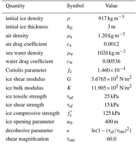
Table 1. Model parameters.
Quantity Symbol Value
initial ice density ρ 917 kg m−3
initial ice thickness h0 3 m
air density ρa 1.20 kg m−3
air drag coefficient ca 0.0012
sea water density ρw 1026 kg m−3
water drag coefficient cw 0.00536
Coriolis parameter fc 1.460×10⁻⁴
ice shear modulus G 3.6765×10⁵N/m2
ice bulk modulus K 11.905×10⁵N/m2
ice tensile strength τnf 25 kPa
ice shear strength τsf 15 kPa
ice compressive strength fc0 125 kPa
ice opening parameter u0 400 m
decohesive parameter κ ln(1−(τsf/τsm)2)
shear magnification τsm 60.0
and observation point-wise, rather we want a metric that tells us the simulation is satisfactory if we get the leads roughly right. That is what our assessment is meant to accomplish.
Levy et al. (2008) define two metrics to evaluate model success in representing lower dimensional features. They treat features through a frequency distribution at predeter-mined spatial regions of the domain. We use one, the RMS index of agreement, in a general skill score (Murphy, 1988): SS=Af−Ar
Ap−Ar
=Af−Ar
1−Ar
. (1)
WhereAis a measure of accuracy and subscripts f, r, and p denote forecast, reference, and perfect, respectively. The ref-erence state used here is that of persistence. The measure of accuracy we consider – the RMS Index of Levy et al. (2008, see Appendix B) – can take a value between 0 (no agree-ment) and 1 (perfect agreement,Ap). As we deal with lower dimensional features for which no climatology (and hence no error correlation information) exists, persistence serves as the reference. Any skill score value greater than zero indi-cates prediction skill over persistence, and can be directly converted to a percentage improvement in skill.
3 An illustrative example
3.1 Experimental design
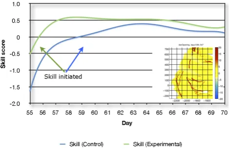
Fig. 2. Skill score (against persistence of observed field shown in
insert) evolution of the control and experimental simulations. A 1-step DA algorithm was implemented on day 54 (23 February 2004) to the experimental run, whereby the ice model state was updated by changing material properties based on agreement of lower dimen-sional features deduced from RGPS data processed to show regions of high deformation (insert). Days are Julian days of 2004.
region of the Beaufort Sea over a time interval of 16 days from day 54 (23 February, insert in Fig. 2) through day 70 (11 March) of 2004. The background mesh size in the MPM calculation is 10 km, with four material points per cell ini-tially. Model parameters include the elastic moduli, ice den-sity, Coriolis parameter, drag coefcients and the parameters in the decohesive model that set the failure strength of ice in tensionτnf and shearτsf, the length scale over which deco-hesion occursu0, and two parameters that describe the shape of the failure surface in stress space,κandτsm(Schreyer et al., 2006, and Appendix A). Values of the parameters used for the simulations are given in Table 1. During this same period in 2004, RADARSAT SAR observations processed through the RADARSAT Geophysical Processor System at 10-km resolution are available daily for validation (middle column in Fig. 3) and assimilation (insert in Fig. 2).
The simulations use the elastic-decohesive constitutive model described above. Six hour wind fields from NCEP reanalysis are used to determine the wind drag and the ocean currents and are updated daily. Both the control and the ex-perimental runs use the same boundary conditions. Bound-aries are either land boundBound-aries, in which case the displace-ment of the ice is zero, or open boundaries in the Beaufort Sea. In the latter case, displacements of boundary points are specified according to their observed values obtained from the RGPS data.
Initial values of all model variables and parameters are also the same, except that the experimental simulation goes through a one-step assimilation during day 54, where infor-mation on the pattern of leads from RGPS at 10-km resolu-tion is used to predispose the model. Initializaresolu-tion includes setting the initial velocity and stress to zero, and the initial
ice thickness uniformly to 3 m. The experimental simulation is further initialized as determined through a kinematic anal-ysis of the RGPS data over one day (Coon et al., 2007; Pe-terson and Sulsky, 2011). Specifically, we determine a jump in displacement and the orientation of this jump that account best for the observed deformation of an RGPS cell. Material points within that cell are initialized to have this initial jump at the observed orientation. The effect of this initialization is to reduce the strength of the ice anisotropically, and to pre-dispose it to continue deforming with this oriented opening provided the forcing is consistent with this deformation.
We run accuracy assessment daily and consider the model response and the impact of the one-step assimilation on sim-ulating LKFs. The assessment consists of determining the accuraciesAfandAragainst the daily observations for both the experimental and control runs using the RMS index of Levy et al. (2008, see Appendix B), and substituting them in the general skill score formulation, Eq. (1) above. We score the different simulations using the RMS Index against the LKFs interpreted from the RGPS observations of the Beau-fort Sea. We consider the agreement in (1) the existence of 100 km×100 km grid cells containing LKFs in the domain; and (2) the existence of 100 km×100 km grid cells contain-ing LKFs at the observed orientation uscontain-ing four cardinal ori-entations in the domain. We thus score M=5 features at N=1, the entire simulated/observed domain (the Beaufort Sea), in Eq. (B1). Here we assume that all weights,wi andωi equal
one. Frequencies are defined in terms of cell counts, and cells with missing data are excluded from the statistics. The impact of the one-step assimilation on simulating LKFs is shown in terms of a skill score in Fig. 2, and visually in Fig. 3.
3.2 Results
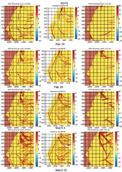
Figure 2 shows the evolution of the skill score with respect to persistence for both the control and experimental simulations for the duration of the simulations from day 55 (24 February 2004), the first day after assimilation of RGPS data (in figure insert) in the experimental run, through day 70 (11 March 2004), the last day of the simulations. The impact of the one step assimilation is evident throughout the entire 16-day simulation, although it is most dramatic during the first week. For visual assessment of the impact that the assim-ilation has on the LKF field throughout the domain, Fig. 3 provides snapshots of that field as simulated in the control and experimental runs, side by side with the observed field at key time steps of the 16-day simulation.
Fig. 3. Comparisons of the experimental (left column) and control (right column) simulations with LKFs interpreted from the RADARSAT
preconditioning, as well as the relatively strong persistence and slow evolution of the lead (LKF) field. The skill score of the experimental run peaks at 0.6 (60% improvement over persistence; 100% improvement over the control run score) on day 58 (27 February), and remains positive for the rest of the simulation, and above 0.5 through day 66 (7 March). In an adaptive assimilation cycle, one may consider another cycle on day 67. The true impact of the assimilation on the model performance is measured relative to the control run. One day following the assimilation, on day 55 (24 Febru-ary), the skill score of the experimental simulation is over 100% higher than that of the control run skill score, even prior to either simulation showing skill relative to persis-tence. At its peak on day 58, the experimental run skill score exhibits an improvement of 100% over the control run’s skill. The control run gains skill relative to persistence on day 59 (28 February; Fig. 3), when it is 80% lower than the skill of the experimental run. The control run skill relative to persis-tence remains positive for the rest of the simulation, peaks at 0.35 on days 63 (4 March in Fig. 3) and 64, but never ex-ceeds the score of 0.5, and, as the skill of both simulations slowly decline at the end of the simulation (e.g., 10 March at the bottom of Fig. 3), it remains consistently at least 10% lower than that of the experimental simulation.
4 Conclusions
An algorithm for model validation and data assimilation that maintains the physical principles embodied in the model and can evaluate and assimilate lower dimensional features (e.g., discontinuities) contained within a bulk simulation is intro-duced and demonstrated with a sea-ice model and with re-motely sensed observations of leads in a one step assimila-tion cycle. An underlying principle of the new algorithm is to use data as a guideline for the model by preconditioning model variables or material properties in a way that leads internal model physics to generate future model states that are in better agreement with the observed state. Similar to four dimensional data assimilation, this procedure produces results that are consistent with internal model physics and dynamics and thus avoids forcing unrealizable model states, largely resolving the problem of initialization. Furthermore, as tested here, this scheme works well for resolving and as-similating lower dimensional features, which do not match the model variables and are not directly measured by the ob-serving system, without the need to transform these features into model variables. Computationally, this scheme is signif-icantly more efficient than four-dimensional assimilation and could be regarded as a simplified 4-D assimilation.
We have tested the new scheme in a sixteen day simulation experiment. In this system, model skill (against persistence) is initiated three days earlier than the skill in the control run with no assimilation, and is consistently higher than the later throughout the simulation. In addition to this shortening of
the model spin up time and the overall higher model skill, the assimilation improves model skill significantly during the first six days. Thus, the new scheme holds the potential of comparable improvements for the assimilation of lower di-mensional features with similar persistence when infrequent observations exist.
In the sea-ice system tested, the properties needing phys-ical adjustments are relatively clear and nudging is a natural implementation choice that is capable of a robust response to the adjustments. However, the same principle of phys-ically based adjustments holds in the general case of other geophysical models and systems, the variables and lower di-mensional features they resolve or represent, as well as in other modes of implementation. Meteorological examples include forecasting precipitation and tropical cyclone trajec-tories (e.g., Kurihara and Ross, 1993). Thus, this scheme could be extended to a generalized multivariate data assim-ilation and fuzzy verification system that would be physi-cally based and capable of extracting lower dimensional in-formation from observations and bulk simulations at differ-ent scales and for differdiffer-ent geophysical (e.g., atmospheric, oceanic, coupled) models containing continuous and lower level features of significance (e.g., fronts, organized convec-tion).
Appendix A
For the purposes of modeling sea ice, a 2-D, plane-stress de-scription of failure has been formulated assuming cracks oc-cur in the plane. The envelope of failure points in stress space is described by a failure function,Fn(σ,n)whereFn<0
im-plies no failure,Fn=0 implies evolving failure andFn>0 is
not allowed. This function is analogous to a plastic yield function in plasticity theories. The subscriptn onFn
indi-cates a separate failure function for each potential crack ori-entation, andFndepends on the stressσ, and the unit normal n to the crack surface. To consider all possible failure direc-tions, a general failure functionF is defined asF=maxnFn.
Many classical failure criteria, such as the Rankine, Tresca and Mohr-Coulomb criteria, are expressed in terms of the traction on the failure surface (i.e., crack surface). The elastic-decohesion model extends these classic criteria by adding two new features: (1) a modification of the Rank-ine criterion for brittle failure to allow for the possibility that a compressive stress component may lower the resistance of the material to brittle failure, and (2) a transition from brittle to ductile failure within one criterion. If a local basis con-sisting of n, the unit normal to the crack, and t, a unit vector tangent to the crack, is introduced, then the traction on the failure surface has normal componentτn=n·σ·n and
tan-gential component τt=t·σ·n. The remaining component
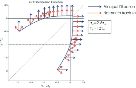
Fig. A1. Failure envelope in principal stress space for the
elastic-decohesive model.
tangential stress,σtt=t·σ·t. The brittle decohesion function is defined as follows
Bn= τn
τnf
−fn
h−σ tti f02
c
+1
, where hxi ≡
x x≥0 0x <0 . (A1) Material parameters are τnf, the tensile or normal failure stress andfc0which denotes the failure stress in uniaxial com-pression. For the moment, takefn=1. The new criterion for
brittle failure isBn=0. The McCauley bracket (h·i) is used
to activate the normal component of stressσtt only if it is negative. If the term involvingσtt were absent then failure would occur when the normal traction on the surface reaches the thresholdτnf, which is the Rankine criterion. With the σttterm, this criterion is analogous to the Rankine criterion in that failure occurs in the direction of maximum principal stress, but the critical value of the normal traction component is potentially reduced whenσttis compressive. The criterion allows for failure even ifτn is negative, and it is this aspect
of the model that allows compressive brittle failure.
Next, brittle and ductile aspects of failure are included by defining the failure function as
F=max
n Fn, Fn
= τ
2
t τ2 sm
+eκBn−1. (A2) The additional material parameter,τsm, is the failure stress in shear when the material is under large compression (τn→
−∞). The parameter,κ, is derived from the condition that under pure shear (Bn= −1), the failure stress isτsf, the fail-ure stress under pfail-ure shear. Ifτnf→ ∞andfc0→ ∞then the criterionF=0 reduces to the pure shear criterion of Tresca. Figure A shows a sketch of the decohesion failure envelope in stress space. The solid line represents the failure envelope F=0. Along this solid line, the blue arrows indicate the di-rection of maximum principal stress and the red arrows indi-cate the normal to the crack surface. Under brittle failure the normal to the crack is in the direction of maximum principal stress. Under ductile and mixed-mode failure the normal to
the crack is at an angle to the direction of maximum princi-pal stress, with two orientations of the crack possible. Of the two, the orientation that preserves the sense of local rotation is chosen. The transition from brittle to ductile failure occurs at a point along the failure envelope determined by the ratio ofτnftoτsf, and thus is a material property.
This failure envelope describes the model for lead initi-ation in the ice. Once the beginning of a crack has been identified, the evolution of the lead is required. The term
decohesion or cohesive crack model refers to the reduction
of the traction on the crack as the crack opens. This behavior is in contrast to Griffith’s model (Griffith, 1921) where the traction is assumed to change discontinuously and instanta-neously from a positive value to zero. Decohesion is included in the model by introducing a softening parameter, analogous to equivalent plastic strain in plasticity models, that drives the traction to zero as a crack continues to open. A dimen-sionless parameter,fn in Eq. (A1), starts with a value unity
for undamaged material and reduces to zero asun, the normal
component of the jump in displacement, increases from zero. The crack is considered completely open whenun reaches
the material-dependent valueu0, at which point the traction on the crack surface has been reduced to zero and a free sur-face is thus formed.
The displacement discontinuity evolves according to a normal flow rule
˙
un= ˙ω ∂F ∂τn
˙
ut= ˙ω ∂F ∂τt
. (A3)
The displacement discontinuity is regularized into an effec-tive decohesion strain, analogous to plastic strain,
˙
ednn= ˙un/L e˙ntd= ˙ut/2L e˙dtt=0 (A4) whereLis a measure of the cell size in numerical simula-tions. (The value ofLis chosen so that the physically correct energy is dissipated during fracture.) The stress is a func-tion of the elastic strain e−ed. Thus, as a specimen of ice is loaded, we typically begin withF <0; the stress is inside the failure envelope. We assume each loading step is elas-tic, giving a trial stress state. If the trial stress is outside the failure envelope (F >0) then a jump in displacement is in-troduced to bringF back to zero. This procedure is identical to standard solution procedures for plasticity. The result is that as a crack opens we predict the amount of both the nor-mal and tangential opening. Once a free surface has formed, the jump in displacement can continue to grow if the crack surfaces continue to separate, and the traction on the surface remains zero.
cracks at a point. If weak areas are known to exist in the ice, the softening parameterfncan be initialized with a value less
than one to account for this information.
Appendix B
The RMS index of agreement (Levy et al., 2008) we use as a measure of accuracy in the skill score, Eq. (1), treats fea-tures through a frequency distribution at predetermined spa-tial segments of the domain. It contains a term with the fa-miliar format of standard error common in routine distance or root mean square error measures used for continuous vari-ables:
IR=1− v u u t
XM
i=1 wi
N
X
j=1 ωjDi,j
/
M
X
i=1 wi
N
X
j=1 ωj
(B1)
wherewi andωj are weights given to the features and the
spatial segments, respectively, andDi,j is a normalized
fre-quency difference function:
Di,j=
pi,j−oi,j2 pi,j+oi,j2
, (B2)
where pi,j and oi,j are the predicted (simulated) and
ob-served feature frequencies (cell count) of featureiin segment j.
Acknowledgements. This work was supported by the Minerals
Management Service and the National Aeronautics and Space Administration (under contract NNH04 CC 45C), and by the National Science Foundation (under grants ARC-0621173 and ATM-0741832).
Edited by: J. Annan
References
Coon, M., Kwok, R., Levy, G., Pruis, M., Schreyer, H., and Sul-sky, D.: Arctic Ice Dynamics Joint Experiment (AIDJEX) as-sumptions revisited and found inadequate, J. Geophys. Res., 112, C11S90, doi:10.1029/2005JC003393, 2007.
Dai, M., Arbetter, T. E., and Meier, W. N.: Data assimilation of sea-ice motion vectors: sensitivity to the parameterization of sea-sea-ice strength, Ann. Glaciol., 44, 357–360, 2006.
Daley, R.: Atmospheric Data Analysis, Published by Cambridge University Press, ISBN: 0521458250, 472 pp., 1992.
Griffith, A. A.: The Phenomena of Rupture and Flow in Solids, Phil. Trans. Royal Soc. London. Series A, 221, 163–198, 1921. Hoke, J. and Anthes, R.: The Initialization of Numerical Models
by a Dynamic Relaxation Technique, Mon. Weather Rev., 104, 1551–1556, 1976.
Hunke, E. C. and Lipscomb, W. H.: CICE: The Los Alamos sea ice model documentation and software users manual, Technical report, Los Alamos National Laboratory, Los Alamos, New Mex-ico, 2004.
Kalnay, E.: Atmospheric Modeling, Data Assimilation, and Pre-dictability, Cambridge University Press, ISBN 0521796296, 9780521796293, 341 pp., 2003.
Kurihara, Y. and Ross, R. J.: An initialization scheme for hurricane models by vortex specification, Mon. Weather Rev., 121, 2030– 2045, 1993.
Kwok, R., Curlander, J. C., McConnell, R., and Pang, S. S.: An ice-motion tracking system at the Alaska SAR facility, IEEE J. Oceanic Eng., 15, 44–54, 1990.
Kwok, R.: The RADARSAT Geophysical Processing System, in: Analysis of SAR Data of the Polar Oceans: Recent Advances, edited by: Tsatsoulis, C. and Kwok, R., Springer-Verlag, Berlin, 235–257, 1998.
Kwok, R.: Deformation of the Arctic Ocean sea ice cover between November 1996 and April 1997: a qualitative survey. In IUTAM Symp. on Scaling Laws in Ice Mechanics and Ice Dynamics, edited by: Dempsey, J. P. and Shen, H. H., Kluwer Academic, Dordrecht, 315–322, 2001.
Levy, G., Coon, M., Nguyen, G., and Sulsky, D.: Metrics for evaluating linear features, Geophys. Res. Let., 35, L21705, doi:10.1029/2008GL035086, 2008.
Lindsay, R. W. and Zang, J.: Assimilation of Ice Concentration in an IceOcean Model, J. Atmos. Ocean. Tech., 23, 742–749, 2006. Mandel, J., Bennethum, L. S., Beezley, J. D., Coen, J. L., Dou-glas, C. C., Kim, M., and Vodacek, A.: A wildland fire model with data assimilation, Math. Comput. Simulat., 79, 504–606, doi:10.1016/j.matcom.2008.03.015, 2008.
Marshall, J., Adcroft, A., Hill, C., Perelman, L., and Heisey, C.: A finite-volume, incompressible Navier-Stokes model for studies of the ocean on parallel computers, J. Geophys. Res., 102(C3), 5753-5766, doi:10.1029/96JC02775, 1997.
Mass, C. F., Ovens, D., Westrick, K., and Colle, B. A.: Does Increasing Horizontal Resolution Produce More Skillful Fore-casts?, B. Am. Meteorol. Soc., 83, 407–430, 2002.
Murphy, A. H.: Skill Scores Based on the Mean Square Error and their relationship to the Correlation Coefficient, Mon. Weather Rev., 116, 2471–2424, 1988.
Peterson, K. and Sulsky, D.: Evaluating Sea Ice Deformation in the Beaufort Sea Using a Kinematic Crack Algorithm with RGPS Data, Chapter 6 in: Remote Sensing of the Changing Oceans, edited by: Tang, D., Gower, J., Levy, G., et al., Springer, ISBN 978-3-642-16540-5, 2011.
Schreyer, H., Munday, L., Sulsky, D., Coon, M., and Kwok, R.: Elastic-Decohesive Constitutive Model for Sea Ice, J. Geophys. Res., 111, C11S26, doi:10.1029/2005JC003334, 2006.
Schulson, E. M.: Compressive shear faults within Arctic sea ice: Fracture on scales large and small, J. Geophys. Res.-Oceans, 109(C7), C07016, doi:10.1029/2003JC002108, 2004.
Sulsky, D., Schreyer, H., Peterson, K., Kwok, R., and Coon, M.: Using the material-point method to model sea ice dynamics, J. Geophys. Res., 112, C02S90, doi:10.1029/2005JC003329, 2007. Talagard, O.: Assimilation of Observations: An Introduction, J.
Meteorol. Soc. Jpn., Special Issue 75(IB), 191–209, 1997. Vukicevic, T. and Bao, J. W.: The Effect of Linearization Errors on