Review on solving the forward problem in EEG source analysis

Open Access

Review

Review on solving the forward problem in EEG source analysis

Hans Hallez*

_{, Bart Vanrumste*}

_{, Roberta Grech}

_{, Joseph Muscat}

_{, Wim De}

Clercq

_{, Anneleen Vergult}

_{, Yves D'Asseler}

_{, Kenneth P Camilleri}

_,

Simon G Fabri

_{, Sabine Van Huffel}

_{and Ignace Lemahieu}

Address: 1_{ELIS-MEDISIP, Ghent University, Ghent, Belgium,} 2_{ESAT, K.U.Leuven, Leuven, Belgium,} 3_{Katholieke Hogeschool Kempen, Geel,}

Belgium, 4_{Department of Mathematics, University of Malta Junior College, Malta,} 5_{Faculty of Engineering, University of Malta, Malta and} 6_{Department of Mathematics, University of Malta, Malta}

Email: Hans Hallez* - [email protected]; Bart Vanrumste* - [email protected];

Roberta Grech - [email protected]; Joseph Muscat - [email protected]; Wim De Clercq - [email protected]; Anneleen Vergult - [email protected]; Yves D'Asseler - [email protected]; Kenneth P Camilleri - [email protected]; Simon G Fabri - [email protected]; Sabine Van Huffel - [email protected]; Ignace Lemahieu - [email protected] * Corresponding authors

Abstract

Background: The aim of electroencephalogram (EEG) source localization is to find the brain areas responsible for EEG waves of interest. It consists of solving forward and inverse problems. The forward problem is solved by starting from a given electrical source and calculating the potentials at the electrodes. These evaluations are necessary to solve the inverse problem which is defined as finding brain sources which are responsible for the measured potentials at the EEG electrodes.

Methods: While other reviews give an extensive summary of the both forward and inverse problem, this review article focuses on different aspects of solving the forward problem and it is intended for newcomers in this research field.

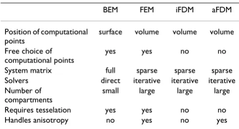
Results: It starts with focusing on the generators of the EEG: the post-synaptic potentials in the apical dendrites of pyramidal neurons. These cells generate an extracellular current which can be modeled by Poisson's differential equation, and Neumann and Dirichlet boundary conditions. The compartments in which these currents flow can be anisotropic (e.g. skull and white matter). In a three-shell spherical head model an analytical expression exists to solve the forward problem. During the last two decades researchers have tried to solve Poisson's equation in a realistically shaped head model obtained from 3D medical images, which requires numerical methods. The following methods are compared with each other: the boundary element method (BEM), the finite element method (FEM) and the finite difference method (FDM). In the last two methods anisotropic conducting compartments can conveniently be introduced. Then the focus will be set on the use of reciprocity in EEG source localization. It is introduced to speed up the forward calculations which are here performed for each electrode position rather than for each dipole position. Solving Poisson's equation utilizing FEM and FDM corresponds to solving a large sparse linear system. Iterative methods are required to solve these sparse linear systems. The following iterative methods are discussed: successive over-relaxation, conjugate gradients method and algebraic multigrid method.

Conclusion: Solving the forward problem has been well documented in the past decades. In the past simplified spherical head models are used, whereas nowadays a combination of imaging modalities are used to accurately describe the geometry of the head model. Efforts have been done on realistically describing the shape of the head model, as well as the heterogenity of the tissue types and realistically determining the conductivity. However, the determination and validation of the in vivo conductivity values is still an important topic in this field. In addition, more studies have to be done on the influence of all the parameters of the head model and of the numerical techniques on the solution of the forward problem.

Published: 30 November 2007

Journal of NeuroEngineering and Rehabilitation 2007, 4:46 doi:10.1186/1743-0003-4-46

Received: 5 January 2007 Accepted: 30 November 2007

This article is available from: http://www.jneuroengrehab.com/content/4/1/46 © 2007 Hallez et al; licensee BioMed Central Ltd.

Introduction

Since the 1930s electrical activity of the brain has been measured by surface electrodes connected to the scalp [1]. Potential differences between these electrodes were then plotted as a function of time in a so-called electroencepha-logram (EEG). The information extracted from these brain waves was, and still is instrumental in the diagnoses of neurological diseases [2], mainly epilepsy. Since the 1960s the EEG was also used to measure event-related potentials (ERPs). Here brain waves were triggered by a stimulus. These stimuli could be of visual, auditory and somatosensory nature. Different ERP protocols are now routinely used in a clinical neurophysiology lab. Researchers nowadays are still searching for new ERP pro-tocols which may be able to distinguish between ERPs of patients with a certain condition and ERPs of normal sub-jects. This could be instrumental in disorders, such as psy-chiatric and developmental disorders, where there is often a lack of biological objective measures.

During the last two decades, increasing computational power has given researchers the tools to go a step further and try to find the underlying sources which generate the EEG. This activity is called EEG source localization. It con-sists of solving a forward and inverse problem. Solving the forward problem starts from a given electrical source con-figuration representing active neurons in the head. Then the potentials at the electrodes are calculated for this con-figuration. The inverse problem attempts to find the elec-trical source which generates a measured EEG. By solving the inverse problem, repeated solutions of the forward problem for different source configurations are needed. A review on solving the inverse problem is given in [3].

In this review article several aspects of solving the forward problem in EEG source localization will be discussed. It is intended for researchers new in the field to get insight in the state-of-the-art techniques to solve the forward prob-lem in EEG source analysis. It also provides an extensive list of references to the work of other researchers.

First, the physical context of EEG source localization will be elaborated on and then the derivation of Poisson's equation with its boundary conditions. An analytical expression is then given for a three-shell spherical head model. Along with realistic head models, obtained from medical images, numerical methods are then introduced that are necessary to solve the forward problem. Several numerical techniques, the Boundary Element Method (BEM), the Finite Element Method (FEM) and the Finite Difference Method (FDM), will be discussed. Also aniso-tropic conductivities which can be found in the white matter compartment and skull, will be handled.

The reciprocity theorem used to speed up the calculations, is discussed. The electric field that results at the dipole location within the brain due to current injection and withdrawal at the surface electrode sites is first calculated. The forward transfer-coefficients are obtained from the scalar product of this electric field and the dipole moment. Calculations are thus performed for each elec-trode position rather than for each dipole position. This speeds up the time necessary to do the forward calcula-tions since the number of electrodes is much smaller than the number of dipoles that need to be calculated.

The number of unknowns in the FEM and FDM can easily exceed the million and thus lead to large but sparse linear systems. As the number of unknowns is too large to solve the system in a direct manner, iterative solvers need to be used. Some popular iterative solvers are discussed such as successive over-relaxation (SOR), conjugate gradient method (CGM) and algebraic multigrid methods (AMG).

The physics of EEG

In this section the physiology of the EEG will be shortly described. In our opinion, it is important to know the underlying mechanisms of the EEG. Moreover, forward modeling also involves a good model for the generators of the EEG. The mechanisms of the neuronal actionpoten-tials, excitatory post-synaptic potentials and inhibitory post-synaptic potentials are very complex. In this section we want to give a very comprehensive overview of the underlying neurophysiology.

Neurophysiology

The brain consists of about 1010 _{nerve cells or neurons.} The shape and size of the neurons vary but they all possess the same anatomical subdivision. The soma or cell body contains the nucleus of the cell. The dendrites, arising from the soma and repeatedly branching, are specialized in receiving inputs from other nerve cells. Via the axon, impulses are sent to other neurons. The axon's end is divided into branches which form synapses with other neurons. The synapse is a specialized interface between two nerve cells. The synapse consists of a cleft between a presynaptic and postsynaptic neuron. At the end of the branches originating from the axon, the presynaptic neu-ron contains small rounded swellings which contain the neurotransmitter substance. Further readings on the anat-omy of the brain can be found in [4] and [5].

can be modeled as a current dipole. The current flow causes an electric field and also a potential field inside the human head. The electric field and potential field spreads to the surface of the head and an electrode at a certain point can measure the potential [2].

At rest the intracellular environment of a neuron is nega-tively polarized at approximately -70 mV compared with the extracellular environment. The potential difference is due to an unequal distribution of Na+_{, K}+ _{and Cl}- _ions across the cell membrane. This unequal distribution is maintained by the Na+ _{and K}+ _{ion pumps located in the} cell membrane. The Goldman-Hodgkin-Katz equation describes this resting potential and this potential has been verified by experimental results [2,6,7].

The neuron's task is to process and transmit signals. This is done by an alternating chain of electrical and chemical signals. Active neurons secrete a neurotransmitter, which is a chemical substance, at the synaptical side. The syn-apses are mainly localized at the dendrites and the cell body of the postsynaptic cell. A postsynaptic neuron has a large number of receptors on its membrane that are sensi-tive for this neurotrans-mitter. The neurotransmitter in contact with the receptors changes the permeability of the membrane for charged ions. Two kinds of

neurotransmit-ters exist. On the one hand there is a neurotransmitter which lets signals proliferate. These molecules cause an influx of positive ions. Hence depolarization of the intra-cellular space takes place. A depolarization means that the potential difference between the intra- and extracellular environment decreases. Instead of -70 mV the potential difference becomes -40 mV. This depolarization is also called an excitatory postsynaptic potential (EPSP). On the other hand there are neurotransmitters that stop the pro-liferation of signals. These molecules will cause an out-flow of positive ions. Hence a hyperpolarization can be detected in the intracellular volume. A hyperpolarization means that the potential difference between the intra- and extracellular environment increases. This potential change is also called an inhibitory postsynaptic potential (IPSP). There are a large number of synapses from different pres-ynaptic neurons in contact with one postspres-ynaptic neuron. At the cell body all the EPSP and IPSP signals are inte-grated. When a net depolarization of the intracellular compartment at the cell body reaches a certain threshold, an action potential is generated. An action potential then propagates along the axon to other neurons [2,6,7].

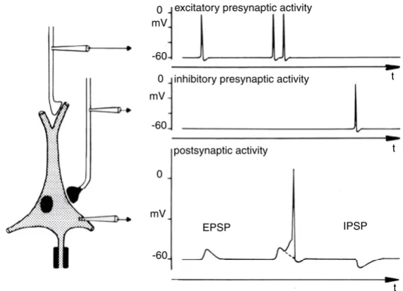
Figure 1 illustrates the excitatory and inhibitory postsyn-aptic potentials. It also shows the generation of an action

Excitatory and inhibitory post synaptic potentials Figure 1

Excitatory and inhibitory post synaptic potentials. An illustration of the action potentials and post synaptic potentials measured at different locations at the neuron. On the left a neuron is displayed and three probes are drawn at the location where the potential is measured. The above picture on the right shows the incoming exitatory action potentials measured at the probe at the top, at the probe in the middle the incoming inhibitory action potential is measured and shown. The neuron processes the incoming potentials: the excitatory action potentials are transformed into excitatory post synaptic potentials, the inhibitory action potentials are transformed into inhibitory post synaptic potentials. When two excitatory post synaptic poten-tials occur in a small time frame, the neuron fires. This is shown at the bottom figure. The dotted line shows the EPSP, in case there was no second excitatory action potential following. From [2].

excitatory presynaptic activity

inhibitory presynaptic activity

postsynaptic activity

EPSP IPSP

t

t

t 0

mV

-60 0

-60 mV

0

potential. Further readings on the electrophysiology of neurons can be found in [2,6].

The generators of the EEG

The electrodes used in scalp EEG are large and remote. They only detect summed activities of a large number of neurons which are synchronously electrically active. The action potentials can be large in amplitude (70–110 mV) but they have a small time course (0.3 ms). A synchronous firing of action potentials of neighboring neurons is unlikely. The postsynaptic potentials are the generators of the extracellular potential field which can be recorded with an EEG. Their time course is larger (10–20 ms). This enables summed activity of neighboring neurons. How-ever their amplitude is smaller (0.1–10 mV) [3,8].

Apart from having more or less synchronous activity, the neurons need to be regularly arranged to have a measura-ble scalp EEG signal. The spatial properties of the neurons must be so that they amplify each other's extracellular potential fields. The neighboring pyramidal cells are organized so that the axes of their dendrite tree are parallel with each other and normal to the cortical surface. Hence, these cells are suggested to be the generators of the EEG.

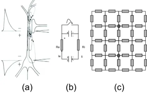
The following is focused on excitatory synapses and EPSP, located at the apical dendrites of a pyramidal cell. The neurotransmitter in the excitatory synapses causes an influx of positive ions at the postsynaptic membrane as illustrated in figure 2(a) and depolarizes the local cell membrane. This causes a lack of extracellular positive ions at the apical dendrites of the postsynaptic neuron. A

redis-tribution of positively charged ions also takes place at the intracellular side. These ions flow from the apical dendrite to the cell body and depolarize the membrane potentials at the cell body. Subsequently positive charged ions become available at the extracellular side at the cell body and basal dendrites.

A migration of positively charged ions from the cell body and the basal dendrites to the apical dendrite occurs, which is illustrated in figure 2(a) with current lines. This configuration generates extracellular potentials. Other membrane activities start to compensate for the massive intrusion of the positively charged ions at the apical den-drite, however these mechanisms are beyond the scope of this work and can be found elsewhere [2,9,10].

A simplified equivalent electric circuit is presented in fig-ure 2(b) to illustrate the initial activity of an EPSP. At rest, the potential difference between the intra- and extracellu-lar compartments can be represented by charged capaci-tors. One capacitor models the potential difference at the apical dendrites side while a second capacitor models the potential difference at the cell body and basal dendrite side. The potential difference over the capacitors is 60 mV. The neurotransmitter causes a massive intrusion of posi-tively charged ions at the postsynaptic membrane at the apical dendrite side. In the equivalent circuit, this is mod-eled by a switch that is closed. The capacitor at the cell body side discharges causing a current flow over the extra-cellular resistor R_e and the intracellular resistor R_i. The repolarization of the cell membrane at the apical side or the initiation of the action potential are not modeled with this simple equivalent electrical circuit.

The capacitors and the switch, in figure 2(b), represent a model of the electrical source at the initial phase of the depolarization of the neuron. They could also be replaced by a time dependent current source, however this repre-sentation is not ideal. The capacitor reprerepre-sentation, for the initial phase of depolarization, fits closer the occurring physical phenomena. The impedance of the tissue in the human head has, for the frequencies contained in the EEG, no capacitive nor inductive component and is hence pure resistive. More advanced equivalent electrical circuits can be found elsewhere [10]. The fact that a current flows through the extracellular resistor indicates that potential differences in the extracellular space can be measured.

A simplified electrical model for this active cell consists of two current monopoles: a current sink at the apical den-drite side which removes positively charged ions from the extracellular environment, and a current source at the cell body side which injects positively charged ions in the extracellular environment. The extracellular resistance R_e

can be decomposed in the volume conductor model in equivalent circuit for a neuron

Figure 2

which the active neuron is embedded, as illustrated in fig-ure 2(c). For further reading on the generation of the EEG one can refer to [11] and [9].

Poisson's equation, boundary conditions and

dipoles

In the previous sections we saw that the generators of the EEG are the synaptic potentials along the apical dendrites of the pyramidal cells of the grey matter cortex. It is impor-tant to notice that the EEG reflects the electrical activity of a subgroup of neurons, especially pyramidal neuron cells, where the apical dendrite is systematically oriented orthogonal to the brain surface. Certain types of neurons are not systematically oriented orthogonal to the brain surface. Therefore, the potential fields of the synaptic cur-rents at different dendrites of neurons van cancel each other out. In that case the neuronal activity is not visible at the surface. Moreover, that actionpotentials, propagat-ing along the axons, have no influence on the EEG. Their short timespan (2 ms) make the chance of generating simultaneous actionpotentials very small [6,12]. In this section, a mathematical approach on the generation of the forward problem is given.

Quasi-static conditions

It is shown in [13] that no charge can be piled up in the conducting extracellular volume for the frequency range of the signals measured in the EEG. At one moment in time all the fields are triggered by the active electric source. Hence, no time delay effects are introduced. All fields and currents behave as if they were stationary at each instance. These conditions are also called quasi-static conditions. They are not static because the neural activity changes with time. But the changes are slow compared to the prop-agation effects.

Applying the divergence operator to the current density Poisson's equation gives a relationship between the potentials at any position in a volume conductor and the applied current sources. The mathematical derivation of Poisson's equation via Maxwell's equations, can be found in various textbooks on electromagnetism [6,10,14]. Pois-son's equation is derived with the divergence operator. In this way the emphasis is, in our opinion, more on the physical aspect of the problem. Furthermore, the concepts introduced in [10,14], such as current source and current sink, are used when applying the divergence operator.

Definition

The current density is a vector field and can be represented by J(x, y, z). The unit of the current density is A/m2_{. The} divergence of a vector field J is defined as follows:

The integral over a closed surface ∂G represents a flux or a current. This integral is positive when a net current leaves the volume G and is negative when a net current enters the volume G. The vector dS for a surface element of ∂G with area dS and outward normal e_n, can also be written as e_ndS. The unit of ∇·J is A/m3 _{and is often called the current} source density which in [15] is symbolized with Im. Gen-erally one can write:

∇·J = I_m. (2)

Applying the divergence operator to the extracellular current density First a small volume in the extracellular space, which encloses a current source and current sink, is investigated. The current flowing into the infinitely small volume, must be equal to the current leaving that volume. This is due to the fact that no charge can be piled up in the extracellular space. The surface integral of equation (1) is then zero, hence ∇·J = 0.

In the second case a volume enclosed by the current sink with position parameters r₁(x₁, y₁, z₁) is assumed. The cur-rent sink represents the removal of positively charged ions at the apical dendrite of the pyramidal cell. The integral of equation (1) remains equal to -I while the volume G in the denominator becomes infinitesimally small. This gives a singularity for the current source density. This sin-gularity can be written as a delta function: -Iδ(r - r₁). The negative sign indicates that current is removed from the extracellular volume. The delta function indicates that current is removed at one point in space.

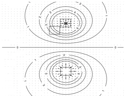
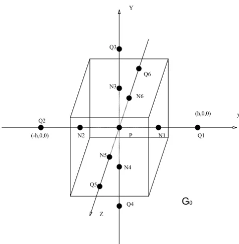
For the third case a small volume around the current source at position r2(x2, y2, z2) is constructed. The current source represents the injection of positively charged ions at the cell body of the pyramidal cell. The current source density equals Iδ(r - r₂). Figure 3 represents the current density vectors for a current source and current sink con-figuration. Furthermore, three boxes are presented corre-sponding with the three cases discussed above.

Uniting the three cases given above, one obtains:

∇·J = Iδ(r - r₂) - Iδ(r - r₁). (3)

Ohm's law, the potential field and anisotropic/isotropic conductivities

The relationship between the current density J in A/m2 _and the electric field E in V/m is given by Ohm's law:

J = σE, (4)

with σ(r) ∈⺢3×3 _{being the position dependent} conductiv-ity tensor given by:

∇ ⋅ =

→

∫

J lim J S

G G G

d

0 1

and with units A/(Vm) = S/m. There are tissues in the human head that have an anisotropic conductivity. This means that the conductivity is not equal in every direction and that the electric field can induce a current density component perpendicular to it with the appropriate σin equation (4).

At the skull, for example, the conductivity tangential to the surface is 10 times [16] the conductivity perpendicular to the surface (see figure 4(a)). The rationale for this is that the skull consists of 3 layers: a spongiform layer between two hard layers. Water, and also ionized parti-cles, can move easily through the spongiform layer, but not through the hard layers [17]. Wolters et al. state that skull anisotropy has a smearing effect on the forward potential computation. The deeper a source lies, the more it is surrounded by anisotropic tissue, the larger the influ-ence of the anisotropy on the resulting electric field. Therefore, the presence of anisotropic conducting tissues compromises the forward potential computation and as a consequence, the inverse problem [18].

White matter consists of different nerve bundles (groups of axons) connecting cortical grey matter (mainly den-drites and cell bodies). The nerve bundles consist of nerve

fibres or axons (see figure 4(b)). Water and ionized parti-cles can move more easily along the nerve bundle than perpendicular to the nerve bundle. Therefore, the conduc-tivity along the nerve bundle is measured to be 9 times higher than perpendicular to it [19,20]. The nerve bundle direction can be estimated by a recent magnetic resonance technique: diffusion tensor magnetic resonance imaging (DT-MRI) [21]. This technique provides directional infor-mation on the diffusion of water. It is assumed that the conductivity is the highest in the direction in which the water diffuses most easily [22]. Authors [23-25] have showed that anisotropic conducting compartments should be incorporated in volume conductor models of the head whenever possible.

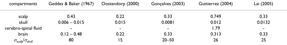
In the grey matter, scalp and cerebro-spinal fluid (CSF) the conductivity is equal in all directions. Thus the place dependent conductivity tensor becomes a place depend-ent scalar σ, a so-called isotropic conducting tissue. The conductivity of CSF is quite accurately known to be 1.79 S/m [26]. In the following we will focus on the conductiv-ity of the skull and soft tissues. Some typical values of con-ductivities can be found in table 1.

The skull conductivity has been subject to debate among researchers. In vivo measurements are very different from in vitro measurements. On top of that, the measurements are very patient specific. In [27], it was stated that the skull conductivity has a large influence on the forward prob-lem.

It was believed that the conductivity ratio between skull and soft tissue (scalp and brain) was on average 80 [20]. Oostendorp et al. used a technique with realistic head models by which they passed a small current by means of 2 electrodes placed on the scalp. A potential distribution

σ

σ σ σ σ σ σ σ σ σ

= ⎡

⎣ ⎢ ⎢ ⎢

⎤

⎦ ⎥ ⎥ ⎥

11 12 13

12 22 23

13 23 33

, (5)

Anisotropic conductivity of the brain tissues Figure 4

Anisotropic conductivity of the brain tissues. The ani-sotropic properties of the conductivity of skull and white matter tissues. The anisotropic properties of the conductiv-ity of skull and white matter tissues. (a) The skull consists of 3 layers: a spongiform layer between two hard layers. The conductivity tangentially to the skull surface is 10 times larger than the radial conductivity. (b) White matter consist of axons, grouped in bundles. The conductivity along the nerve bundle is 9 times larger than perpendicular to the nerve bun-dle.

The current density and equipotential lines in the vicinity of a dipole

Figure 3

The current density and equipotential lines in the vicinity of a dipole. The current density and equipotential lines in the vicinity of a current source and current sink is depicted. Equipotential lines are also given. Boxes are illus-trated which represent the volumes G.

5

4

3

2

2

1

1 1

0 0

1

1

1

2

2 3

3

4

is then generated on the scalp. Because the potential val-ues and the current source and sink are known, only the conductivities are unknown in the head model and equa-tion (4) can be solved toward σ. Using this technique they could estimate the skull-to-soft tissue conductivity ratio to be 15 instead of 80 [28]. At the same time, Ferree et al. did a similar study using spherical head models. Here, skull-to-soft tissue conductivity was calculated as 25. It was shown in [29] that using a ratio of 80 instead of 16, could yield EEG source localization errors of an average of 3 cm up to 5 cm.

One can repeat the previous experiment for a lot of differ-ent electrode pairs and an image of the conductivity can be obtained. This technique is called electromagnetic impedance tomography or EIT. In short, EIT is an inverse problem, by which the conductivities are estimated. Using this technique, the skull-to-soft tissue conductivity ratio was estimated to be around 20–25 [30,31]. However in [30], it was shown that the skull-to-soft tissue ratio could differ from patient to patient with a factor 2.4. In [32], maximum likelihood and maximum a posteriori tech-niques are used to simultaneously estimate the different conductivities. There they estimated the skull-to-soft tis-sue ratio to be 26.

Another study came to similar results using a different technique. In Lai et al., the authors used intracranial and scalp electrodes to get an estimation of the skull-to-soft tissue ratio conductivity. From the scalp measures they estimated the cortical activity by means of a cortical imag-ing technique. The conductivity ratio was adjusted so that the intracranial measurements were consistent with the result of the imaging from the scalp technique. They resulted in a ratio of 25 with a standard deviation of 7. One has to note however that the study was performed on pediatric patients which had the age of between 8 and 12. Their skull tissue normally contains a larger amount of ions and water and so may have a higher conductivity than the adults calcified cranial bones [33]. In a more experimental setting, the authors of [34] performed con-ductivity measures on the skull itself in patients undergo-ing epilepsy surgery. Here the authors estimated the skull conductivity to be between 0.032 and 0.080 S/m, which

comes down to a soft-tissue to skull conductivity of 10 to 40.

Poisson's equation

The scalar potential field V, having volt as unit, is now introduced. This is possible due to Faraday's law being zero under quasi-static conditions (∇ × E = 0) [35]. The link between the potential field and the electric field is given utilizing the gradient operator,

E = -∇V. (6)

The vector ∇V at a point gives the direction in which the scalar field V, having volt as its unit, most rapidly increases. The minus sign in equation (6) indicates that the electric field is oriented from an area with a high potential to an area with a low potential. Figure 3 also illustrates some equipotential lines generated by a current source and current a sink.

When equation (2), equation (4) and equation (6) are combined, Poisson's differential equation is obtained in general form:

∇·(σ∇(V)) = -I_m. (7)

For the problem at hand, equation (3), equation (4) and equation (6) are combined yielding:

∇·(σ∇(V)) = -Iδ(r - r₂) + Iδ(r - r₁). (8)

In the Cartesian coordinate system equation (8) becomes for isotropic conductivities:

and for anisotropic conductivities:

∂ ∂

∂ ∂ + ∂∂

∂ ∂ + ∂∂

∂

∂ = − − − −

+

x V

x y

V

y z

V

z I x x y y z z

I

(σ ) (σ ) (σ ) δ( 2) (δ 2) (δ 2) δδ(x−x1) (δ y−y1) (δ z−z1)

(9)

Table 1: The reference values of the absolute and relative conductivity of the compartments incorporated in the human head.

compartments Geddes & Baker (1967) Oostendorp (2000) Gonçalves (2003) Guttierrez (2004) Lai (2005) scalp 0.43 0.22 0.33 0.749 0.33 skull 0.006 – 0.015 0.015 0.0081 0.012 0.0132 cerebro-spinal fluid - - - 1.79

-brain 0.12 – 0.48 0.22 0.33 0.313 0.33

The potentials V are calculated with equations (8), (9) or (10) for a given current source density I_m, in a volume conductor model, e.g. in our application, the human head. Compartments in which all conductivities are equal, are called homogeneous conducting compart-ments.

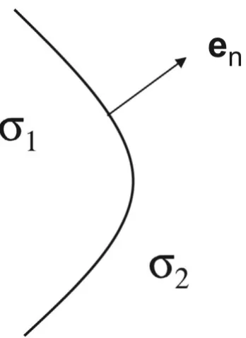
Boundary conditions

At the interface between two compartments, two bound-ary conditions are found. Figure 5 illustrates such an inter-face. A first condition is based on the inability to pile up charge at the interface. All charge leaving one ment through the interface must enter the other compart-ment. In other words, all current (charge per second) leaving a compartment with conductivity σ₁ through the interface enters the neighboring compartment with con-ductivity σ₂:

where en is the normal component on the interface.

In particular no current can be injected into the air outside the human head due to the very low conductivity of the air. Therefore the current density at the surface of the head reads:

Equations (11) and (12) are called the Neumann bound-ary condition and the homogeneous Neumann boundbound-ary condition, respectively.

The second boundary condition only holds for interfaces not connected with air. By crossing the interface the potential cannot have discontinuities,

V₁ = V₂. (13)

This equation represents the Dirichlet boundary condi-tion.

The current dipole

Current source and current sink inject and remove the same amount of current I and they represent an active pyramidal cell at microscopic level. They can be modeled as a current dipole as illustrated in figure 6(a). The posi-tion parameter r_dip of the dipole is typically chosen half way between the two monopoles.

The dipole moment d is defined by a unit vector e_d (which is directed from the current sink to the current source) and a magnitude given by d = ||d|| = I·p, with p the distance between the two monopoles. Hence one can write:

d = I·pe_d. (14)

It is often so that a dipole is decomposed in three dipoles located at the same position of the original dipole and each oriented along one of the Cartesian axes. The magni-tude of each of these dipoles is equal to the orthogonal projection on the respective axis as illustrated in figure 6(b). one can write:

d = d_xe_x + d_ye_y + d_ze_z, (15)

with ex, ey and ez being the unit vectors along the three axes. Furthermore, d_x, d_y and d_z are often called the dipole components. Notice that Poisson's equation (8) is linear.

σ11 σ22 σ33 σ12 σ13 σ23

2 2

2 2

2

2 2

2 2 2

∂ ∂ +

∂ ∂ +

∂ ∂ +

∂ ∂ ∂ +

∂ ∂ ∂ +

∂

V

x V

y V

z

V x y

V x z

V V y z

x y z

V

x x

∂ ∂ ⎛

⎝ ⎜ ⎜

⎞ ⎠ ⎟ ⎟

+ ∂⎛ _∂ + ∂_∂ + ∂_∂ ⎝

⎜ ⎞

⎠

⎟∂_∂ + ∂_∂ + ∂_∂

σ11 σ12 σ13 σ12 σ22

yy z

V

y x y z

V z

I x x

+ ∂_∂ ⎛

⎝

⎜ ⎞

⎠

⎟∂_∂ + ∂⎛ _∂ + ∂_∂ + ∂_∂ ⎝

⎜ ⎞

⎠ ⎟∂_∂ = − −

σ σ σ σ

δ

23 13 23 33

( 22) (δy−y2) (δz−z2)+Iδ(x−x1) (δy−y1) (δz−z1).

(10)

J e J e

e e

1⋅ = 2⋅

∇ ⋅ = ∇ ⋅

n n

n n

V V

,

(σ_{1 1}) (σ_{2 2}) , (11)

J e

e

1⋅ =

⋅ ∇ ⋅ =

n

n

V

0 0

1 1

,

(σ ) . (12)

The boundary between two compartments Figure 5

Due to a dipole at a position r_dip and dipole moment d, a potential V at an arbitrary scalp measurement point r can be decomposed in:

V(r, rdip, d) = dxV(r, rdip, ex) + dyV(r, rdip, ey) + dzV(r, rdip, ez). (16)

A large group of pyramidal cells need to be more or less synchronously active in a cortical patch to have a measur-able EEG signal. All these cells are furthermore oriented with their longitudinal axis orthogonal to the cortical sur-face. Due to this arrangement the superposition of the individual electrical activity of the neurons results in an amplification of the potential distribution. A large group of electrically active pyramidal cells in a small patch of cortex can be represented as one equivalent dipole on macroscopic level [36,37]. It is very difficult to estimate the extent of the active area of the cortex as the potential distribution on the scalp is almost identical to that of an equivalent dipole [38].

General algebraic formulation of the forward problem

In symbolic terms, the EEG forward problem is that of finding, in a reasonable time, the scalp potential g(r, r_dip, d) at an electrode positioned on the scalp at r due to a sin-gle dipole with dipole moment d = de_d (with magnitude d

and orientation e_d), positioned at r_dip. This amounts to solving Poisson's equation to find the potentials V(r) on

the scalp for different configurations of r_dip and d. For multiple dipole sources, the electrode potential would be . In practice,

one calculates a potential between an electrode and a erence (which can be another electrode or an average ref-erence).

For N electrodes and p dipoles:

where i = 1,...,p and j = 1,...,N. Here V is a column vector.

For N electrodes, p dipoles and T discrete time samples:

where V is now the matrix of data measurements, G is the gain matrix and D is the matrix of dipole magnitudes at different time instants.

More generally, a noise or perturbation matrix n is added,

V = GD + n.

In general for simulations and to measure noise sensitiv-ity, noise distribution is a gaussian distribution with zero mean and variable standard deviation. However in reality, the noise is coloured and the distribution of the frequency depends on a lot of factors: patient, measurement setup, pathology,....

A general multipole expansion of the source model

Solving the inverse problem using multiple dipole model requires the estimation of a large number of parameters, 6 for each dipole. Given the use of a limited number of EEG electrodes, the problem becomes underdetermined. In this case, regularization techniques have to be applied, but this leads to oversmoothed source estimations. On the other hand, the use of a limited number of dipoles (one, two or three) leads to very simplified sources, which are very often ambiguous and cause errors due to simpli-fied modelling. The dipole model as a source is a good model for focal brain activity.

V g dip i g d

i

dip i

i

i i i

( )r =

∑

∑

V r

r

r r ed r r ed

= ⎡ ⎣ ⎢ ⎢ ⎢ ⎤ ⎦ ⎥ ⎥ ⎥ = V V g g N

dip dipp p

( )

( )

( , , ) ( , , )

1 1 1 1 1

# " # % # gg g d d

N dip N dipp p p (r ,r ,e_d) (r ,r ,e_d)

1 1 1 " # ⎡ ⎣ ⎢ ⎢ ⎢ ⎢ ⎤ ⎦ ⎥ ⎥ ⎥ ⎥ ⎡ ⎣ ⎢ ⎢ ⎢ ⎤ ⎦ ⎥ ⎥ ⎥⎥= ⎡ ⎣ ⎢ ⎢ ⎢ ⎤ ⎦ ⎥ ⎥ ⎥

G r r({ ,j dip,ed}) p i i d d 1 # V r r r r

G r r = ⎡ ⎣ ⎢ ⎢ ⎢ ⎤ ⎦ ⎥ ⎥ ⎥ =

V V T

V _N V _N T

j dipi

( , ) ( , )

( , ) ( , )

({ , ,

11 1

1

"

# % #

"

e

e_di G r r _i e_di D

d d

d d

T

p p T

j dip

}) ({ , , })

, ,

, ,

1 1 1

1 " # % # " ⎡ ⎣ ⎢ ⎢ ⎢ ⎤ ⎦ ⎥ ⎥ ⎥= (17) The dipole parameters

Figure 6

A multipole expansion is an alternative (first introduced by [39]), which is based on a spherical harmonic expan-sion of the volume source, which is not necessarily focal. It provides the added model flexibility needed to account for a wide range of physiologically plausible sources, while at the same time keeping the number of estimation parameters sufficiently low. In fact, The zeroth-order and first-order terms in the expansion are called the monopole and dipole moment, respectively. A quadrupole is a higher order term and is generated by two equal and oppositely oriented dipoles whose moments tend to infinity as they are brought infinitesimally close to each other. An octapole consists of two quadrupoles brought infinitesimally close to each other and so on. It can be shown that if the volume G containing the active sources

I_sv(r') is limited in extent, the solution to Poisson's equa-tion for the potential V may be expanded in terms of a multipole series:

V = Vmonopole + Vdipole + Vquadrupole + Voctapole + Vhexadecpole + ... (18)

where V_quadrupole is the potential field caused by the quad-rupole. In practice, a truncated multipole series is used up to a quadrupole, because the contribution to the electrode potentials by a octapole or higher order sources rapidly decreases when the distance between electrode and source is increasing. The use of quadrupoles can sound plausible in the following case: A traveling action potential causes a depolarization wave through the axon, followed by a repolarization wave. These two phenomenon produce two opposite oriented dipoles very close to each other [40]. In sulci, pyramidal cells are oriented toward each other, which makes the use of quadrupole also reasona-ble. However, the skull causes a strong attenuation of the electrical field created by the source. Therefore, even a quadrupole has low contribution to the electrode poten-tials of the EEG, created by the volume current in the extracellular region. In EEG and ECG multiple dipoles of dipole layers are preferred over a multipole. Multipoles are popular in magnetoencephalographic (MEG) source localization, because of its low sensitivity to the skull con-ductivity [6,10,41,42].

Solving the forward problem

Dipole field in an infinite homogeneous isotropic conductor

The potential field generated by a current dipole with dipole moment d = de_d at a position r_dip in an infinite con-ductor with conductivity σ, is introduced. The potential field is given by:

with r being the position where the potential is calculated. Assume that the dipole is located in the origin of the Car-tesian coordinate system and oriented along the z-axis. Then it can be written:

where θrepresents the angle between the z-axis and r and

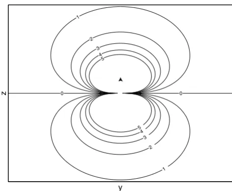
r = ||r||. An illustration of the electrical potential field caused by dipole is shown in figure 7.

Equation (20) shows that a dipole field attenuates with 1/

r2_{. It is significant to remark that V, from equation (19),} added with an arbitrary constant, is also a solution of Poisson's equation. A reference potential must be chosen. One can choose to set one electrode to zero or one can opt for average referenced potentials. The latter result in elec-trode potentials that have a zero mean.

The spherical head model

The first volume conductor models of the human head consisted of a homogeneous sphere [43]. However it was soon noticed that the skull tissue had a conductivity which was significantly lower than the conductivity of scalp and brain tissue. Therefore the volume conductor model of the head needed further refinement and a three-shell concentric spherical head model was introduced. In this model, the inner sphere represents the brain, the intermediate layer represents the skull and the outer layer

V dip

dip

dip

( , , ) ( )

|| ||

,

r r d d r r

r r

= ⋅ −

−

4πσ 3 (19)

V d d

r

z

( , ,r 0 e )= cosθ ,

πσ

4 2

(20)

The equipotential lines of a dipole Figure 7

The equipotential lines of a dipole. The equipotential lines of a dipole oriented along the z-axis. The numbers cor-respond to the level of intensity of the potential field gener-ated of the dipole. The zero line divides the dipole field into two parts: a positive one and a negative one.

y

z

1

2

3 4

5

5 4

3

2

1

represents the scalp. For this geometry a semi-analytical solution of Poisson's equation exists. The derivation is based on [44,45]. Consider a dipole located on the z-axis and a scalp point P, located in the xz-plane, as illustrated in figure 8. The dipole components located in the xz-plane i.e. d_r the radial component and d_t the tangential compo-nent, are also shown in figure 8. The component orthogo-nal to the xz-plane, does not contribute to the potential at scalp point P due to the fact that the zero potential plane of this component traverses P. The potential V at scalp point P for the proposed dipole is given by:

with gi given by:

Where:

d_r is the radial component (3 × 1-vector in meters),

d_t is the tangential component (3 × 1-vector in meters),

R is the radius of the outer shell (meters),

S is the conductivity of scalp and brain tissue (Siemens/ meter),

X is the ratio between the skull and soft tissue conductivity (unitless),

b is the relative distance of the dipole from the centre (unitless),

θis the polar angle of the surface point see figure 8 (radi-ans),

P_i(·) is the Legendre polynomial,

is the associated Legendre polynomial,

i is an index,

i₁ equals 2i + 1,

r1 is the radius of the inner shell (in meters),

r₂ is the radius of the middle shell (in meters),

f₁ equals r₁/R (unitless) and

f₂ equals r₂/R (unitless).

Equation (21) gives the scalp potentials generated by a dipole located on the z-axis, with zero dipole moment in the y direction. To find the scalp potentials generated by an arbitrary dipole, the coordinate system has to be rotated accordingly. Typical radii of the outer boundaries of the brain, skull and scalp compartments are equal to 8 cm, 8.5 cm and 9.2 cm, respectively [46]. An illustration of a typical spherical head model is shown in figure 8. These radii can be altered to fit a sphere more to the human head. The infinite series of equation (21) is often truncated. If the first 40 terms are used, the maximum scalp potential obtained with the truncated series, devi-ates less than 0.1% from the case where 100 terms are applied, for dipoles with a radial position smaller than 95% of the maximum brain radius.

There are also semi-analytical solutions available for lay-ered spheroidal anisotropic volume conductors [47-49]. Here the conductivity in the tangential direction can be chosen differently than in the radial direction of the sphere. Analytic solutions also exist for prolate and oblate spheroids or eccentric spheres [50-52].

V

SR

X i

gi i i b id P d P

i

r i t i

i

= +

+ − +

= ∞ 1

4 2

2 1 3 1

1 1

1

π θ θ

( )

( ) [ (cos ) (cos )],

∑

∑

(21)

g i X i iX

i X i X i f f i X

i

i i

= + +

+ + + − + + − − −

[( 1) ][ ] ( )[( ) ]( ) ( ) (

1 1 1 1 1 2 1

2

1 1 _{ff f} i

1/ 2) .1 (22)

P_i1( )⋅

The three-shell concentric spherical head model Figure 8

The three-shell concentric spherical head model. The dipole is located on the z-axis and the potential is measured at scalp point P located in the xz-plane.

8.5cm 9.2cm

8.0cm

q

X Z

P dr

Variants of the three-shell spherical head model, such as the Berg approximation [53], in which a single-sphere model is used to approximate a three- (or four-) layer sphere, have also been used to improve further the com-putational efficiency of multi-layer spherical models.

Recently however, it is becoming more apparent that the actual geometry of the head [54-56] together with the var-ying thickness and curvatures of the skull [57,58], affects the solutions appreciably. So-called real head models are becoming much more common in the literature, in con-junction with either boundary-element, finite-element, or finite-difference methods. However, the computational requirements for a realistic head model are higher than that for a multi-layer sphere.

An approach which is situated between the spherical head model approaches and realistic ones is the sensor-fitted sphere approach [59]. Here a multilayer sphere is fitted to each sensor located on the surface of a realistic head model.

The boundary element method

The boundary element method (BEM) is a numerical tech-nique for calculating the surface potentials generated by current sources located in a piecewise homogeneous vol-ume conductor. Although it restricts us to use only iso-tropic conductivities, it is still widely used because of its low computational needs. The method originated in the field of electrocardiography in the late sixties and made its entrance in the field of EEG source localization in the late eighties [60]. As the name implies, this method is capable of providing a solution to a volume problem by calculat-ing the potential values at the interfaces and boundary of the volume induced by a given current source (e.g. a dipole). The interfaces separate regions of differing con-ductivity within the volume, while the boundary is the outer surface seperating the non-conducting air with the conducting volume.

In practice, a head model is built from surfaces, each encapsulating a particular tissue. Typically, head models consist of 3 surfaces: brain-skull interface, skull-scalp interface and the outer surface. The regions between the interfaces are assumed to be homogeneous and isotropic conducting. To obtain a solution in such a piecewise homogenous volume, each interface is tesselated with small boundary elements.

The integral equations describing the potential V(r) at any point r in a piecewise volume conductor V were described in [61-63]:

where σ0 corresponds to the medium in which the dipole source is located (the brain compartment) and V₀(r) is the

potential at r for an infinite medium with conductivity σ₀

as in equation (19). and are the conductivities of

the, respectively, inner and outer compartments divided by the interface S_j. dS is a vector oriented orthogonal to a surface element and ||dS|| the area of that surface element.

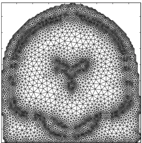
Each interface S_j is digitized in triangles, (see figure

9) and in each triangle centre the potentials are calculated using equation (23). The integral over the surface Sj is transformed into a summation of integrals over traingles on that surface. The potential values on surface S_j can be written as

where the integral is over , the j-th triangle on the

surface S_j, R is the number of interfaces in the volume. An exact solution of the integral is generally not possible,

therefore an approximated solution on surface S_k

may be defined as a linear combination of

simpleba-sis functions

V

k _k

V j j

k _k

V d

( ) ( )

_

( )

|| ||

r r r r r

r r S

= −_{+ +} +

− +

− + + ′ ′−′−

2 0 1

2 3

0

σ

σ σ π

σ σ

σ σ r′∈ jj

=

∫

∑

j R

j 1

,

(23)

σ_j− _σ j +

NSj

V

r r

V k k

r r

V d

( ) ( ) _ ( )

|| ||

r r r r r

r r S

= −_{+ +} + − +

− + + ′ ′−′−

2 0 1

2 3

0 σ

σ σ π

σ σ

σ σ Δ_{Sk j} kk

Sk

j N

k R

,

,

∫

∑

∑

(24) ΔS kj,

Vk( )r

N_S k

Vk V h_ik _i

i N_Sk

j

( )r = ( ).r

=

∑

Example mesh of the human head used in BEM Figure 9

The coefficients represent unknowns on surface S_k

whose values are determined by constraining to sat-isfy (24) at discrete points, also known as collocation points. Moreover, equation (24) can be rewritten as

This equation can be transformed into a set of linear equa-tions:

V = BV + V₀, (27)

where V and V₀ are column vectors denoting at every node the wanted potential value and the potential value in an infinite homogeneous medium due to a source, respec-tively. B is a matrix generated from the integrals, which depends on the geometry of the surfaces and the conduc-tivities of each region.

Determination of the elements of the matrix B is compu-tationally intensive and there exist different approaches for their computation. The integral in equation (23) is also often called the solid angle [62,64,65]. The basis functions h_i(r) can be defined in several ways. The "con-stant-potential" approach for triangular elements uses basis functions defined by

where Δi denotes the ith planar triangle on the tesselated surface. The collocation points are typically the centroids of the surface elements and the unknown potentials V are the potentials at each triangle [66]. The "linear potential" approach uses basis functions defined by

where ri, rj, rk are the nodes of the triangle and the triple scalar product is defined as [r_i r_j r_k] = det(r_i, r_j, r_k). The nota-tion Δ_i(jk) is used to indicate any triangle for which one ver-tex is defined by the vector r_i, the remaining two vertices denoted as r_j and r_k. The function h_i(r) attains a value of unity at the ith vertex and drops linearly to zeros at the opposite edge of all triangles to which r_i is a vertex. In this case, the collocation points are the vertices of the elements [66]. The approaches can be expanded into higher-order elements [67]. Gençer and Tanzer investigated quadratic

and cubic element types and concluded that these gave superior results to models with linear elements [68].

Barnard et al. [64] showed that the potentials in equation (27) are only defined up to an additive constant. Hence, equation (27) has no unique solution. This ambiguity can be removed by deflation, which means that B must be replaced by

where e is a vector with all its N (the total number of unknowns) components equal to one. The deflated equa-tion

V = CV + V₀, (31)

possesses a unique solution which is also a solution to the orignal equation (27). If I denotes the N × N identity matrix and A represents I - C then

V = A-1_V

0. (32)

This equation can be solved using direct or iterative solv-ers. Direct solvers are especially usefull when the matrix A is relatively small because of a coarse grid. If one wants to use a fine grid, then iterative methods should be used. The use of multiple deflations during the iterations can signif-icantly increase the convergence time to the solution of equation (31) [69].

A typical head model for solving the forward problem involves 3 layers: the brain, the skull and the scalp. The conductivity of the skull is lower than the conductivity of brain and scalp. If βis defined as the ratio of the skull con-ductivity to the brain concon-ductivity Meijs et al. showed that an accurate solution of equation (23) is difficult to obtain for small β(β< 0.1). The large difference between the con-ductivities will cause an amplification of the numerical errors in the calculation. To solve this problem, the Iso-lated Problem Approach (IPA) can be used (also called Isolated Skull Approach), which was introduced by Hämäläinen and Sarvas [70]. Assume the labeling of the compartments as Cscalp, Cskull and Cbrain and Sscalp as the outer interface, S_skull as the interface between C_skull and

C_brain and S_brain as the interface between C_brain and C_skull. The IPA uses the following decomposition of the potential val-ues:

V(r) = V'(r) + V''(r) (33)

where V'' is the potential on surface S_brain when the head is a homogeneous brain region, thus omitting the skull and

V_ik

V( )x

V

r r

V k k

r r

V_ik h

i N

i

Sk

( ) ( ) _ ( )

|

r _{= −} r r r r

+ + +

− +

− + +

∑

2 0 1

2

0

1 σ

σ σ π

σ σ

σ σ || ||

.

, ′−

∫

∑

∑

S_k

3

1 1

d

Sk j Sk

j N

k R

Δ

(26)

h_i i

i

( )r r

r

= ∈

∉ ⎧ ⎨ ⎩ 1 0

Δ

Δ (28)

h

j k i j k

i

i jk

i jk ( )

[ ]

[ ] ( )

( ) r

r r r

r r r r

r

= ∈

∉ ⎧

⎨ ⎪

⎩ ⎪

Δ

Δ 0

(29)

C= −B 1 ee

N

T

scalp compartments. V' is the correction term. When V is written like above, equation (32) can be written as

Because V'' is zero on the interfaces S_scalp and S_skull, V' con-tains the potential values on the outer surface. The IPA is based on the more accurate solution of the right-hand side term . An accurate solution can be obtained by setting

to the following

where , and are the potentials at respectively

the brain-skull surface, the skull-scalp surface and the

outer surface. This imposes that has to be calculated.

This can be done by solving the potentials at Sbrain with the scalp and skull compartments omitted. The increase in accuracy comes at a small cost of computational speed. A weighted IPA approach was developed by Fuchs et al. [71]. The IPA approach was extended to multi-sphere models by Gençer and Akahn-Acar [72]. The calculation of the forward problem involves every node on the mesh, making it very computation intesive. Accelerated BEM computes the node potentials on a small subset of nodes corresponding to the electrode positions [73].

To improve the localization accuracy, one can locally refine the mesh. Yvert et al. showed that if the dipole is at 2 cm below the surface, a mesh of 0.5 triangles/cm2 _is needed to have acceptable results. However, for shallow dipoles (between 2 mm and 20 mm below the brain sur-face) a mesh density of 2–6 triangles per cm2 _{is needed to} obtain comparable results. Of course, the area in the mesh that has to be refined, has to be defined.

A main disadvantage using BEM in the EEG forward prob-lem is that in all aforementioned impprob-lementations the precision drops when the distance of the source to one of the surfaces becomes comparable to the size of the trian-gles in the mesh. Kybic et al. presented a new framework based on a theorem that characterizes harmonic functions defined on the complement of a bounded smooth surface

[74]. Using this framework, they proposed a symmetric formulation. The main benefit of this approach is that the error increases much less dramatically when the current sources approach a surface where the conductivity is dis-continuous. In another paper by the same authors, a fast multipole acceleration was used to overcome the com-plexity of the symmetric formulation [75]. A recent article of the same authors demonstrates that the framework allows the use of more realistical head models, which don't have to be nested. In nested head models, an inner interface is completely enveloped by an outer interface. Non-nested compartments are compartments that are not part of the brain, but part of the head (such as eyes, sinuses,...) [76].

The finite element method

Another method to solve Poisson's equation in a realistic head model is the finite element method (FEM). The Galerkin approach [77] is used to equation (7) with boundary conditions (11), (12), (13). First, equation (7) is multiplied with a test function φ and then integrated over the volume G representing the entire head. Using Green's first identity for integration:

in combination with the boundary conditions (12), yields the 'weak formulation' of the forward problem:

If (v, w) = ∫_Gv(x, y, z)w(x, y, z)dG and a(u, v) = -(∇v, σ∇u), this can be written as:

a(V, φ) = (I_m, φ) (38)

The entire 3D volume conductor is digitized in small ele-ments. Figure 10 illustrates a 2D volume conductor digi-tized with triangles.

The computational points can be identified with

the vertices of the elements (n is the number of vertices). The unknown potential V(x, y, z) is given by

where denotes a set of test functions also called

basis functions. They have a local support, i.e. the area in ′ + ′′ =

′ = − ′′

′ = ′

−

−

−

V V A V

V A V AV

V A V

1 0 1

0 1

0

( )

.

(34)

′ V0 ′ V₀

′ = ′ ′ ′ ⎛

⎝ ⎜ ⎜ ⎜ ⎜

⎞

⎠ ⎟ ⎟ ⎟ ⎟ =

−

+ ′′ ⎛

⎝ ⎜ ⎜ ⎜ ⎜ V

V

V

V

V

V

V V

0

2 1 01

0 2

03

01

0 2

0 3

0 3 β

β

β β

β ⎜⎜⎜

⎞

⎠ ⎟ ⎟ ⎟ ⎟ ⎟⎟

, (35)

V₀1 V₀2 V₀3

′′ V₀3

∇ ⋅ ∇ = ∇ ⋅ − ∇ ∇

∫

∫

∫

(36)

− ∇ ⋅ ∇

∫

∫

G G m

(37)

{ }V_{i i}n₌₁

V x y z Vi i x y z

i n

( , , )= ( , , ),

=

∑

(39)

which they are non-zero is limited to adjacent elements. Moreover, the basis functions span a space of piecewise polynomial functions.

Furthermore, they have the property that they are each equal to unity at the corresponding computational point and equal to zero at all other computational points. Sub-stituting (39) in equation (38) produces n equations in n

unknowns V = [V₁...V_n]T ∈⺢n×1_:

Due to the local support of the basis function, each equa-tion consists only of a linear combinaequa-tion of Vi's and its adjacent computational points. Hence the system A ∈

⺢n×n_{, A}

ij = a(φi, φj) is sparse. In matrix notation one can obtain:

A·V = I, (42)

with I ∈⺢n×1 _{being the column vector of the source terms} obtained by the right hand side of equation (41).

An important consideration in finite-element methods is how to represent a dipole source in the model.

• The obvious direct method is to represent a dipole using a pair of fixed voltage conditions of opposite polarity applied to two adjacent nodes [78].

• Another method is to embed a dipole source in the ele-ment basis functions. When the dipole lies along the edge of an element, this approach reduces to the simple idea of using two concentrated sources at either end of that edge [78].

• A third formulation is to separate the field in two parts – one part is a standard field produced by an ideal dipole in an infinite homogeneous domain and the other part is a solution in the closed sourceless domain under bound-ary conditions that correct the current movement across boundaries between regions of different conductivity [78].

• In the Laplace formulation, a small volume containing the dipole is removed and fixed boundary conditions are applied at all nodes on the surface of the removed vol-ume. This can be interpreted as replacing current sources by an estimate of the equivalent voltage sources [78].

• A fifth formulation is the blurred dipole model, where source and sink monopoles are divided over the neigh-bouring nodes. In most cases the source and sink monop-oles do not coincide with nodes of the FEM-mesh. Therefore a way to represent the dipole is by a summation of monopoles placed at neighbouring nodes [79].

A comparison of the resulting surface potentials using the first four methods with the exact analytical solution using ideal dipoles (with an infinitesimal separation between the two poles, an infinite total current exiting one pole and entering the other, and a finite dipole moment, which is the product of the current and separation) in a 4-layer concentric sphere was made in [78]. It was found that the third formulation gives the best performance for both transverse and radial dipoles (followed by the Laplace for-mulation for radial dipoles).

A recent innovation [80,81] is to consider current monop-oles (point sources/sinks) instead of dipmonop-oles. Using the equivalent-current inverse solution (ECS) approach for p

grid locations, only p variables need to be determined in the inverse problem, whereas if a dipole is placed at each of the p grid locations, the solution space consists of 3p

unknown variables because each dipole has 3 directional components. This results in an advantage of using current monopoles instead of current dipoles as demonstrated in [81] where it is shown that the time required to calculate

a V_{i i j} I

i n

m j

( φ φ, ) ( , ),φ

=

∑

1

(40)

a _{i j}V I

i n

i m j

( , )φ φ ( , )φ =

∑

1

(41) Example mesh in 2D used in FEM

Figure 10