A comprehensive benchmarking system for evaluating global vegetation models

(1)

Biogeosciences, 10, 3313–3340, 2013 www.biogeosciences.net/10/3313/2013/ doi:10.5194/bg-10-3313-2013

EGU Journal Logos (RGB)

Advances in

Geosciences

Open Access

Natural Hazards

and Earth System

Sciences

Open Access

Annales

Geophysicae

Open Access

Nonlinear Processes

in Geophysics

Open Access

Atmospheric

Chemistry

and Physics

Open Access

Atmospheric

Chemistry

and Physics

Open Access

Discussions

Atmospheric

Measurement

Techniques

Open Access

Atmospheric

Measurement

Techniques

Open Access

Discussions

Biogeosciences

Open Access Open Access

Biogeosciences

Discussions

Climate

of the Past

Climate

of the Past

Discussions

Earth System

Dynamics

Earth System

Dynamics

Discussions

Geoscientific

Instrumentation

Methods and

Data Systems

Open Access

_{Geoscientific}

Instrumentation

Methods and

Data Systems

Open Access

Discussions

Geoscientific

Model Development

Geoscientific

Model Development

Discussions

Hydrology and

Earth System

Sciences

Open Access

Hydrology and

Earth System

Sciences

Open Access

Discussions

Ocean Science

Discussions

Solid Earth

Discussions

The Cryosphere

Discussions

Natural Hazards

and Earth System

Sciences

Open Access

Discussions

A comprehensive benchmarking system for evaluating global

vegetation models

D. I. Kelley1, I. C. Prentice1,2, S. P. Harrison1,3, H. Wang1,4, M. Simard5, J. B. Fisher5, and K. O. Willis1 1_{Department of Biological Sciences, Macquarie University, North Ryde, NSW 2109, Australia}

2_{Grantham Institute for Climate Change, and Department of Life Sciences, Imperial College, Silwood Park Campus, Ascot}

SL5 7PY, UK

3_{Geography & Environmental Sciences, School of Human and Environmental Sciences, Reading University, Whiteknights,}

Reading, RG6 6AB, UK

4_{State Key Laboratory of Vegetation and Environmental Change, Institute of Botany, Chinese Academy of Science,}

Xiangshan Nanxincun 20, 100093 Beijing, China

5_{Jet Propulsion Laboratory, California Institute of Technology, Pasadena, CA 91109, USA}

Correspondence to: D. I. Kelley ([email protected])

Received: 20 July 2012 – Published in Biogeosciences Discuss.: 9 November 2012 Revised: 5 March 2013 – Accepted: 7 March 2013 – Published: 17 May 2013

Abstract. We present a benchmark system for global

veg-etation models. This system provides a quantitative eval-uation of multiple simulated vegetation properties, includ-ing primary production; seasonal net ecosystem production; vegetation cover; composition and height; fire regime; and runoff. The benchmarks are derived from remotely sensed gridded datasets and site-based observations. The datasets al-low comparisons of annual average conditions and seasonal and inter-annual variability, and they allow the impact of spatial and temporal biases in means and variability to be assessed separately. Specifically designed metrics quantify model performance for each process, and are compared to scores based on the temporal or spatial mean value of the observations and a “random” model produced by bootstrap resampling of the observations. The benchmark system is ap-plied to three models: a simple light-use efficiency and water-balance model (the Simple Diagnostic Biosphere Model: SDBM), the Lund-Potsdam-Jena (LPJ) and Land Processes and eXchanges (LPX) dynamic global vegetation models (DGVMs). In general, the SDBM performs better than either of the DGVMs. It reproduces independent measurements of net primary production (NPP) but underestimates the ampli-tude of the observed CO2seasonal cycle. The two DGVMs

show little difference for most benchmarks (including the inter-annual variability in the growth rate and seasonal cy-cle of atmospheric CO2), but LPX represents burnt fraction

demonstrably more accurately. Benchmarking also identified several weaknesses common to both DGVMs. The bench-marking system provides a quantitative approach for evalu-ating how adequately processes are represented in a model, identifying errors and biases, tracking improvements in per-formance through model development, and discriminating among models. Adoption of such a system would do much to improve confidence in terrestrial model predictions of cli-mate change impacts and feedbacks.

1 Introduction

Dynamic global vegetation models (DGVMs) are widely used in the assessment of climate change impacts on ecosys-tems, and feedbacks through ecosystem processes (Cramer et al., 1999; Scholze et al., 2006; Sitch et al., 2008; Scheiter and Higgins, 2009). However, there are large differences in model projections of the vegetation response to scenarios of future changes in atmospheric CO2 concentration and

(2)

processes in a particular model that need improvement; and checking that improvements in one part of a model do not compromise performance in another.

Benchmarking is a routine component in the assessment of climate-model performance, including investigation of pa-rameter uncertainties (e.g. Murphy et al., 2004; Piani et al., 2005) and multi-model comparison (Randall et al., 2007; Re-ichler and Kim, 2008), and is used both to inform model de-velopment (e.g. Jackson et al., 2008) and to interpret the re-liability of projections of future climate (e.g. Shukla et al., 2006: Hall and Qu, 2006). In recent years, there has been considerable effort spent on the development of standard metrics for climate-model evaluation (Taylor, 2001; Gleck-ler et al., 2008: Lenderink, 2010; Moise and Delage, 2011; Yokoi et al., 2011). In comparison, there has been little quan-titative assessment of DGVM performance under recent con-ditions. Although most studies describing vegetation-model development provide some assessment of the model’s pre-dictive ability by comparison with observational datasets (e.g. Sitch et al., 2003; Woodward and Lomas, 2004; Prentice et al., 2007), such comparisons often focus just on one as-pect of the model where recent development has taken place (e.g. Gerten et al., 2004; Arora and Boer, 2005; Zeng et al., 2008; Thonicke et al., 2010; Prentice et al., 2011). It has not been standard practice to track improvements in (or degrada-tion of) general model performance caused by new develop-ments.

A benchmarking system should facilitate more compre-hensive model evaluation, and help to make such tracking routine. The land modelling community has recently recog-nized the need for such a system (e.g. the International Land Model Benchmarking Project, ILAMB: http://www.ilamb. org/), and some recent studies have designed and applied benchmarking systems. Blyth et al. (2009, 2011) compared results of the JULES land-surface model with site-based wa-ter and CO2 flux measurements and satellite vegetation

in-dices, quantifying the difference between model output and observations using root mean squared error (RMSE) as a metric. Beer et al. (2010) used a gridded dataset of gross pri-mary productivity (GPP), derived from up-scaling GPP from the FLUXNET network of eddy covariance towers (Jung et al., 2009, 2010) to assess and compare the Lund-Potsdam-Jena (LPJ), LPJmL, ORCHIDEE, CLM-CN and SDGVM models. Bonan et al. (2011) evaluated latent heat fluxes with the tower-derived gridded GPP dataset (Beer et al., 2010) to evaluate the calibration of the CLM4 model. Cadule et al. (2010) used the model-to-data deviation, normalised standard deviation and Pearson’s correlation to quantify the “distance” between simulated and observed CO2

concentra-tion and applied these to compare three coupled climate– vegetation models that incorporate two DGVMs: TRIFFID and ORCHIDEE. All of these studies focus on a very lim-ited number of simulated processes, and use metrics that are difficult to interpret across processes and models. Randerson et al. (2009) introduced a more systematic framework to

as-sess and compare the performance of two biogeochemical models (CLM-CN and CASA’) against net primary produc-tion (NPP) and CO2concentration data, including the

defi-nition of comparison metrics tailored to the benchmark ob-servations and a composite skill score that combined met-ric scores for each observation into an overall measure of model performance. The Randerson et al. (2009) composite score was a weighted combination of scores across differ-ent metrics, where the weights were based on a qualitative and necessarily somewhat subjective assessment of the “im-portance” and uncertainty of each process (Randerson et al., 2009). Luo et al. (2012) recommended the development of a working benchmarking system for vegetation models that in-corporates some of the approaches used in these various stud-ies including a set of standard target datasets for benchmarks, a scoring system; and a way of comparing across model pro-cesses in order to evaluate model strengths and weaknesses to guide model development. Luo et al. (2012) reject the idea of a single composite metric because of the subjectivity in-volved in choices of relative weightings.

Our purpose here is to demonstrate a benchmarking system including multiple observational datasets and transparent metrics of model performance with respect to individual processes. We have tested the system on three vegetation models to demonstrate the system’s capabilities in comparing model performance, assigning a level of confidence to the models’ predictions of key ecosystem properties, assessing the representation of different model processes and identifying deficiencies in each model.

2 Materials and methods

2.1 Principles

The benchmarking system consists of a collection of datasets, selected to fulfil certain criteria and to allow system-atic evaluation of a range of model processes, and metrics, designed with the characteristics of each benchmark dataset in mind. We selected site-based and remotely sensed obser-vational datasets that, as far as possible, fulfil the following requirements:

– They should be global in coverage or, for site-based

data, they should sample reasonably well the differ-ent biomes on each contindiffer-ent. This criterion excludes “campaign mode” measurements, and datasets assem-bled only for one continent or region.

– They should be independent of any modelling approach

(3)

used by Randerson et al. (2009), or remotely sensed evapotranspiration (e.g. Fisher et al., 2008, 2011; Mu et al., 2011). It allows use of flux measurements and CO2inversion products, but excludes, for example, the

up-scaled GPP used by Beer et al. (2010).

– They should be available for multiple years and

sea-sonal cycles to allow assessment of modelled seasea-sonal and inter-annual variation, for variables that change on these time scales.

– Datasets should be freely available, so that different

modelling groups can evaluate their models against the same benchmarks.

The selected datasets (Table 1) provide information for the following: fAPAR, the fractional coverage of different plant life and leaf forms, GPP and NPP, height of the canopy, fire, as burnt fraction; runoff, as river discharge, and seasonal and inter-annual variation in atmospheric CO2concentration

(Fig. 1):

– fAPAR is the fundamental link between primary

pro-duction and available energy (Monteith, 1972). It mea-sures the seasonal cycle, inter-annual variability and trends of vegetation cover. Of all ecosystem properties derived from spectral reflectance measurements, fAPAR is closest to the actual measurements.

– Fractional cover of different life forms and leaf forms

provides basic information about vegetation structure and phenology.

– GPP and NPP are the two fundamental measures of

pri-mary production.

– Vegetation height is a key variable for characterising

vegetation structure, function and biomass.

– Remotely sensed data on fire (as fractional burnt area)

have been available for a few years (e.g. Carmona-Moreno et al., 2005; Giglio et al., 2006). The latest dataset (Giglio et al., 2010; van der Werf et al., 2010) is derived from active fire counts and involves empir-ical (biome-dependent) modelling to translate between active fire counts and burned area. Our criteria exclude the use of the accompanying fire CO2emissions

prod-uct (van der Werf et al., 2010), however, as this de-pends strongly on the use of a particular biogeochemical model.

– Annual runoff is an indicator of ecosystem function, as

it represents the spatial integration of the difference be-tween precipitation and evapotranspiration – the latter primarily representing water use by vegetation. It is a sensitive indicator, because a small proportional error in modelled evapotranspiration translates into a larger pro-portional error in runoff (Raupach et al., 2009). Runoff

is measured independently of meteorological data by gauges in rivers.

– Atmospheric CO2 concentration is measured at high precision at a globally distributed set of stations in re-mote locations (distant from urban and transport cen-tres of CO2emission). The pattern of the seasonal cycle

of atmospheric CO2concentration at different locations

provides information about the sources and sinks of CO2in the land biosphere (Heimann et al., 1998), while

the inter-annual variability of the increase in CO2

pro-vides information about CO2uptake at the global scale.

Ocean impacts on the seasonal cycle are small (Nevi-son et al., 2008). For inter-annual variability we use inversion products which selectively remove the ocean contribution (about 20 % of the signal: Le Qu´er´e et al., 2003).

All remotely sensed data were re-gridded to a 0.5◦_resolution grid and masked to a land mask common to all three models. Data–model comparison metrics were designed to be easy to implement, intuitive to understand, and comparable across multiple benchmarked processes. Metric scores for compar-ison of models with these datasets were compared against scores from two null models: one corresponding to the ob-servational mean and the other obtained by randomly resam-pling the observations.

To demonstrate whether the benchmark system fulfilled the functions of evaluating specific modelled processes and discriminating between models, we applied it to three global models: a simple light-use efficiency and water-balance model introduced by Knorr and Heimann (1995), known as the Simple Diagnostic Biosphere Model (SDBM: Heimann et al., 1998) and two DGVMs. The SDBM is driven by ob-served precipitation, temperature and remotely sensed obser-vations of fAPAR. The model has two tunable global param-eters representing light-use efficiency under well-watered conditions, and the shape of the exponential temperature de-pendence of heterotrophic respiration. The DGVMs are the Lund-Potsdam-Jena (LPJ) model (version 2.1: Sitch et al., 2003, as modified by Gerten et al., 2004) and the Land sur-face Processes and eXchanges (LPX) model (Prentice et al., 2011). LPX was developed from LPJ-SPITFIRE (Thonicke et al., 2010), and represents a further refinement of the fire module in LPJ-SPITFIRE.

2.2 Benchmark datasets

2.2.1 fAPAR

(4)

[image:4.595.53.548.81.435.2]

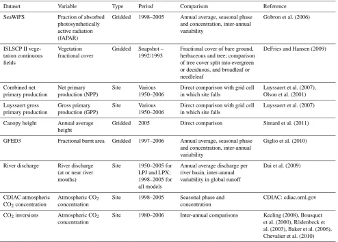
Table 1. Summary description of the benchmark datasets.

Dataset Variable Type Period Comparison Reference

SeaWiFS Fraction of absorbed photosynthetically active radiation (fAPAR)

Gridded 1998–2005 Annual average, seasonal phase and concentration, inter-annual variability

Gobron et al. (2006)

ISLSCP II vege-tation continuous fields

Vegetation fractional cover

Gridded Snapshot – 1992/1993

Fractional cover of bare ground, herbaceous and tree; comparison of tree cover split into evergreen or deciduous, and broadleaf or needleleaf

DeFries and Hansen (2009)

Combined net primary production

Net primary production (NPP)

Site Various 1950–2006

Direct comparison with grid cell in which site falls

Luyssaert et al. (2007), Olson et al. (2001)

Luyssaert gross primary production

Gross primary production (GPP)

Site Various 1950–2006

Direct comparison with grid cell in which site falls

Luyssaert et al. (2007)

Canopy height Annual average height

Gridded 2005 Direct comparison Simard et al. (2011)

GFED3 Fractional burnt area Gridded 1997–2006 Annual average, seasonal phase and concentration, inter-annual variability

Giglio et al. (2010)

River discharge River discharge (at or near river mouths)

Site 1950–2005 for LPJ and LPX; 1998–2005 for all models

Annual average discharge per river basin, inter-annual variability in global runoff

Dai et al. (2009)

CDIAC atmospheric CO₂concentration

Atmospheric CO₂ concentration

Site 1998–2005 Seasonal phase and concentration

CDIAC: cdiac.ornl.gov

CO₂inversions Atmospheric CO₂ concentration

Site 1980–2006 Inter-annual comparisons Keeling (2008), Bousquet et al. (2000), R¨odenbeck et al. (2003), Baker et al. (2006), Chevalier et al. (2010)

obtained for times when the solar incidence angle is>50◦. This limitation mostly affects cells at high latitudes, or with complex topography, during winter. Cells where fAPAR val-ues could not be obtained for any month were excluded from all comparisons. Annual fAPAR, which is the ratio of total annual absorbed to total annual incident PAR, is not the same as the average of the monthly fAPAR. True annual fAPAR was obtained by averaging monthly values weighted by PAR. Monthly PAR values were calculated using Clime Research Unit (CRU) TS3.1 monthly fractional cloud cover (Jones and Harris, 2012) as described in Gallego-Sala et al. (2010). Monthly and annual fAPAR values were used for annual av-erage, inter-annual variability and seasonality comparisons. The monthly fAPAR data are used as a driver for the SDBM, but as a benchmark for the DGVMs.

2.2.2 Vegetation cover

Fractional cover data (Table 1) were obtained from Interna-tional Satellite Land-Surface Climatology Project (ISLSCP) II vegetation continuous field (VCF) remotely sensed prod-uct (Hall et al., 2006; DeFries and Hansen, 2009 and

refer-ences therein). The VCF product provides separate informa-tion on life form, leaf type and leaf phenology at 0.5◦ reso-lution for 1992–1993. There are three categories in the life-form dataset: tree (woody vegetation>5 m tall), herbaceous (grass/herbs and woody vegetation<5 m), and bare ground cover. Leaf type (needleleaf or broadleaf) and phenology (de-ciduous or evergreen) is only given for cells that have some tree cover. Tree cover greater than 80 % is not well delineated due to saturation of the satellite signal, whereas tree cover of less than 20 % can be inaccurate due to the influence of soil and understorey on the spectral signature (DeFries et al., 2000).

(5)

[image:5.595.62.539.59.334.2]

Fig. 1. Illustration of the benchmark datasets: ISLSCP II continuous vegetation fields based on a snapshot for 1992–1993 (DeFries and Hansen, 2009) give the proportions of (a) woody vegetation>5 m in height (tree), (b) grass/herb and woody vegetation<5 m (herbaceous), and (c) bare ground; for areas with tree cover, the datasets also give the proportion of (d) evergreen, (e) deciduous, (f) broadleaf and (g) needleleaf; (i) annual average fAPAR value for 1998–2005 from SeaWiFS (Gobron et al., 2006); (j) annual average burnt fraction for 1997– 2006 from the GFED3 dataset (Giglio et al., 2010); (k) sites with measurements of net primary production, NPP and (l) measurements of gross primary production, GPP are both from the Luyssaert et al. (2007) dataset; (m) global atmospheric CO₂concentrations for 1980–2005 based on inversion datasets (Bousquet et al., 2000; R¨odenbeck et al., 2003; Baker et al., 2006; Chevalier et al., 2010); (n) annual average river runoff from 1950–2005 from the Dai et al. (2009) dataset, displayed over associated GRDC basins (http://www.bafg.de/GRDC); and (m) vegetation height based on a snapshot from 2005 (Simard et al., 2011). Hashed area in (g) shows areas without comparison data.

2.2.3 NPP

The NPP dataset (Table 1) was created by combining site data from the Luyssaert et al. (2007) and the Ecosystem Model/Data Intercomparison (EMDI: Olson et al., 2001) databases. We exclude sites from managed or disturbed envi-ronments; i.e. we do not use class B records from EMDI, and we exclude sites classified as “managed”, “recently burnt”, “recently cut clear”, “fertilized” or “irrigated” in Luyssaert et al. (2007) . The Luyssaert et al. (2007) data used here are all from woody biomes, and all but two of the EMDI data used are from grasslands. The NPP estimates in Luyssaert et al. (2007) were obtained by summing direct measurements of the following: (a) year-round leaf litter collection, (b) stem and branch NPP (from measurements of basal area, scaled using allometric equations), (c) fine root NPP from soil cor-ing, isotopic turnover estimates or upscaling of root length production as observed in mini-rhizotrons, or indirectly via soil respiration, and (d) understorey NPP through destructive harvests. The uncertainty in the NPP estimate is provided for each site, and ranges from 110–656 g C m−2 depending on

the latitude, data collection and analysis methods. The NPP estimates in the EMDI database were collected from the pub-lished literature, and therefore derived using a similar variety of methodologies as used in the Luyssaert et al. (2007) com-pilation. The individual studies were divided into 2 classes based on an assessment of data quality. Here, we use only the top class (class A), which represents sites that are geolocated, have basic environmental metadata, and have NPP measure-ments on both above- and below-ground components. The EMDI database does not include estimates of the uncertain-ties associated with individual sites.

2.2.4 GPP

(6)

2.2.5 Canopy height

The forest canopy height dataset (Table 1; Simard et al., 2011) is derived from Ice, Cloud, and land Elevation Satel-lite/Geoscience Laser Altimeter System (ICESat/GLAS) es-timates of canopy height and its relationship with forest type, MODIS percent tree cover product (MOD44B), elevation and climatology variables (annual mean and seasonality of precipitation and temperature). Only GLAS and MODIS data from 2005 were used. The canopy height product was vali-dated with globally distributed field measurements. Canopy height ranges from 0 to 40 m, and uncertainty is of the order of 6 m (root mean squared error). There are no estimates of the uncertainty for individual grid cells.

2.2.6 Burnt fraction

Burnt fraction data (Table 1) were obtained for each month from 1997–2006 from the third version of the Global Fire Emissions Database (GFED3: Giglio et al., 2010). Burnt fraction was calculated from high-resolution, remotely sensed daily fire activity and vegetation production using sta-tistical modelling. Quantitative uncertainties in the estimates of burnt fraction, provided for each grid cell, are a combina-tion of errors in the higher resolucombina-tion fire activity data and errors associated with the conversion of these maps to low-resolution burnt area.

2.2.7 River discharge

River discharge (Table 1) was obtained from monthly mea-surements at station gauges between 1950 and 2005 (Dai et al., 2009). Dai et al. (2009) use a model-based infill-ing procedure in their analyses, but the dataset used here is based only on the gauge measurements. The basin associated with gauges close to a river mouth was defined using infor-mation from the Global Runoff Data Centre (GRDC: http: //www.bafg.de/GRDC). Average runoff for the basin was ob-tained by dividing discharge by total basin area. Although in-dividual gauge measurements may have measurement errors of the order of 10–20 %, the use of spatially integrated dis-charge values means that the uncertainties are considerably less than this (Dai et al., 2009). Annual average and inter-annual variability comparisons for runoff were made only for years in which there were 12 months of data, to avoid seasonal biases.

2.2.8 CO2concentration

CO2concentration (Table 1) data were taken from 26 Carbon

Dioxide Information Analysis Center (CDIAC: cdiac.ornl. gov) stations (Fig. 3) for seasonal cycle comparisons. For inter-annual comparisons, we used several inversion products (Bousquet et al., 2000; R¨odenbeck et al., 2003; Baker et al., 2006; Keeling, 2008; Chevalier et al., 2010), processed as in Prentice et al. (2011). The inversions are designed to isolate

the component of variability in the CO2growth rate due to

land–atmosphere exchanges. The differences between these inversions (maximum difference 3.8 ppm) give a measure of the associated uncertainty.

2.3 Metrics

Many measures with different properties are used in the geosciences literature to compare modelled and observed quantities. These typically fall into three categories: non-normalised metrics; metrics non-normalised by observational un-certainty; and metrics normalised by observational variance. Non-normalised metrics, which include RMSE (used e.g. by Blyth et al., 2009, 2011) and mean squared error (MSE), can-not be compared directly between different variables as they are in different units. Metrics normalised by observational uncertainty require uncertainty estimates to be given for each site/grid cell in a dataset. Most of the datasets used in this study do not have such estimates, ruling out the use of met-rics normalised by observational uncertainty. We therefore use metrics normalised by observational variance, allowing metrics based on both mean deviations (modulus-based) and mean squared deviations as alternative “families”.

The mean, variance and standard deviation provide a basic measure of global agreement between model and observa-tion. Our basic normalised metrics for taking the geographic patterning into account in data–model comparisons of annual averages or totals were the normalised mean error (NME) and the normalised mean squared error (NMSE) (for defini-tions, limits and applicadefini-tions, see Table 2):

NME=X

i|yi−xi|/ X

i|xi− ¯x|, (1)

NMSE=X

i(yi−xi)

2_/X

i(xi− ¯x)

2_, ₍₂₎

(7)

[image:7.595.44.548.115.387.2]

Table 2. Summary description of the benchmark metrics.yi is the modelled andxi is the corresponding observed value in cell or sitei, and ¯

xis the mean observed value across all grid cells or sites.ωiis the modelled phase, andϕi is the observed phase.qijis the modelled andpi observed proportion of itemjin cell or sitei.

Metric Equation Limits Use in this study

Normalised mean error (NME)

Normalised mean squared error (NMSE)

NME=P

i|yi−xi|/Pi|xi− ¯x|

NMSE=P

i(yi−xi)2/Pi(xi− ¯x)2

0 – Perfect agreement

1 – Model performs as well as observational mean

2 – complete disagreement for step 3

Infinity – complete disagree-ment for step 1 and 2

For burnt fraction and fAPAR: annual averages, phase concentration, inter-annual variability.

For runoff: annual averages, inter-annual variability

For CO2: phase concentration

For NPP, GPP and height: annual averages

Mean phase difference (MPD)

MPD=(1/π )arccos

cos(ωi−φi) /n 0 – in phase

1 – 6 months out (out of phase)

Assessing difference in seasonality for fAPAR, burnt fraction and CO₂

Manhattan metric (MM)

Squared chord dis-tance (SCD)

MM=P ij

qij−pij

/n

SCD=P ij

√ qij−

√ pij2/n

0 – Perfect agreement

2 – Perfect disagreement

Vegetation cover comparisons for life forms, tree, grassland, bare ground, evergreen vs. deciduous tree and broadleaf vs. needleleaf tree.

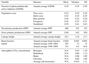
Table 3. Mean, absolute variance (as defined in Eq. 3) and standard deviation (SD) of the annual average values of observations. The variance for most variables is from the long-term mean of the gridded or site data, whereas CO2is the variance of the inter-annual differences.

Variable Measure Mean Variance SD

Fraction of photosynthetically Annual average fAPAR 0.18 0.18 0.20 active radiation (fAPAR)

Vegetation cover Tree cover 0.22 0.22 0.26

Herb cover 0.52 0.25 0.29

Bare ground 0.20 0.24 0.30

Evergreen 0.44 0.33 0.37

Needleleaf 0.59 0.41 0.43

Net primary production (NPP) Annual average NPP 688 242 325

Gross primary production (GPP) Annual average GPP 1540 642 820

Canopy height Annual average canopy height 18.3 11.8 13.7

Burnt fraction Annual average burnt fraction 0.028 0.043 0.094

runoff Annual average 1950–2005 307 12 15

Annual average 1998–2005 331 8.4 10.6

Atmospheric CO2concentration Bousquet N/A 0.93 1.10

R¨odenbeck N/A 0.89 1.13

Baker N/A 0.86 1.09

Chevalier N/A 0.86 1.06

[image:7.595.119.478.447.705.2]

(8)

2.3.1 Annual average

Annual average comparisons were made using the mean, mean deviation (Eq. 3) and standard deviation of simulated and observed values (Table 3). NME and NMSE compar-isons were conducted in three stages: (1)xi andyitake mod-elled and observed values; (2)xi andyi become the differ-ence between observed or modelled values and their respec-tive means (xi→xi− ¯x); and (3)xi andyi from step 2 are divided by either the mean deviation or standard deviation (xi→xi/d(x)):

for NME, dNME(x)=

X

i|xi− ¯x|/n; (3)

for NMSE, dNMSE(x)=

q_X

i(xi− ¯x)

2_/n. ₍₄₎

Stage 2 removes the influence of the mean, and stage 3 re-moves the influence of the variability, on the measure. The NMSE at stage 3 is related to the correlation coefficient (Barnston et al., 1992). Van Oijen et al. (2011) showed that MSE can be decomposed into three elements similar to stage 1, 2 and 3 here, but as MSE is not normalised the decompo-sition is not directly applicable for this study.

2.3.2 Inter-annual variability

Inter-annual variability comparisons were made by calculat-ing global values for each year of the model output and obser-vations, and comparing them using Eqs. (1) and (2), but with

yi now being the global sum of modelled values for yeari, andxi the corresponding observed value. Only stage 2 and 3 comparisons were made, as the stage 1 provides no extra information from the annual-average comparisons. Stage 3 comparison measures whether a model has the correct tim-ing or phastim-ing of annual peaks and troughs. For inter-annual CO2 concentration, the observational data were

de-trended to remove the effect of anthropogenic emissions.

2.3.3 Seasonality

The seasonal expression of change can be characterised in terms of the length and timing of the season, as well as the magnitude of differentiation between seasons. For example, in simulating the fire regime at a particular place, the length of the fire season and the time that fires occur are as impor-tant as correctly predicting the area burnt. Seasonality com-parisons were conducted in two parts: seasonal concentra-tion (which is inversely related to season length) and phase (expressing the timing of the season). Each simulated or ob-served month was represented by a vector in the complex plane, the length of the vector corresponding to the magni-tude of the variable for each month and the directions of the vector corresponding to the time of year:

θt =2π (t−1) /12, (5)

where θt is the direction corresponding to month t, with month 1 (January) arbitrarily set to an angle of zero. A mean vectorLwas calculated by averaging the real and imaginary parts of the 12 vectors,xt.

Lx= X

txtcos(θt) and Ly= X

txtsin(θt) (6) The length of the mean vector divided by the annual value stands for seasonal concentration,C; its direction stands for phase,P:

C= q

L2_x+L2_y P

txt

; (7)

P =arctan Lx/Ly. (8)

Thus, if the variable is concentrated all in one month, sea-sonal concentration is equal to 1 and the phase corresponds to that month. If the variable is evenly spread over all months, then concentration is equal to zero and phase is undefined. If either modelled or observed values have zero values for all months in a given cell or site, then that cell/site is not in-cluded in the comparisons. Concentration comparisons use Eqs. (1) and (2) and steps 1, 2 and 3. Modelled and observed phase are compared using mean phase difference (MPD): MPD=(1/π )arccos [cos(ωi−φi) /n], (9) whereωiis the modelled phase, andϕiis the observed phase. The measure can be interpreted as the average timing error, as a proportion of the maximum error (6 months). For seasonal CO2concentrations, where the data are monthly deviations

from the mean CO2, we compared the seasonal amplitude

in-stead of seasonal concentration by comparing the simulated and observational sum of the absolute CO2deviation for each

month using Eqs. (1) and (2).

2.3.4 Relative abundance

Relative abundance was compared using the Manhattan met-ric (MM) and squared chord distance (SCD) (Gavin et al., 2003; Cha, 2007):

MM=X

ij

qij−pij

/n; (10)

SCD=X ij

√ qij−

√ pij,

2

/n (11)

(9)

2.3.5 Null models

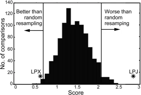
To facilitate interpretation of the scores, we compared each benchmark dataset to a dataset of the same size, filled with the mean of the observations (Table 4). We also com-pared each benchmark dataset with “randomized” datasets (Table 4). This was done using a bootstrapping procedure (Efron, 1979; Efron and Tibshirani, 1993), whereby we con-structed a dataset of the same dimensions as the benchmark set, filled by randomly resampling the cells or sites in the original dataset with replacement. We created 1000 random-ized datasets to estimate a probability density function of their scores (Fig. 2). Models are described as better/worse than randomized resampling if they were less/more than two standard deviations from the mean randomized score.

As NME and MM are the sum of the absolute spatial vari-ation between the model and observvari-ations, the comparison of scores obtained by two different models shows the rela-tive magnitude of their biases with respect to the observa-tions, or how much “better” one model is than another. If a model has an NME score of 0.5, for example, its match to the observations is 50 % better than the mean of the data score of 1.0. Similarly, when this model is compared to a model with an NME score of 0.75, it can be described as 33 % better than the second model as its average spatial er-ror is 0.5/0.75 = 67 % the size. Conversely, the second model would need to reduce its errors/improve by 33 % in order to provide as good a match to observations as the first.

2.4 Models

2.4.1 SDBM

The SDBM simulates NPP and heterotrophic respiration (Rh)

as described in Knorr and Heimann (1995) while the embed-ded water-balance calculation models evapotranspiration and therefore implicitly runoff. NPP is obtained from a simple re-lationship:

NPP=ε·fapar·Ipar·α, (12)

whereεis light-use efficiency, set at 1 g C MJ−1; Ipar is in-cident PAR; andαis the ratio of actual to equilibrium evap-otranspiration, calculated as in Prentice et al. (1993) and Gallego-Sala et al. (2010).Rhwas calculated as a function

of temperature and water availability and for each cell is as-sumed to be equal to NPP each year (i.e. assuming the respir-ing pool of soil carbon is in equilibrium):

Rh=β·QT /₁₀10·α, (13)

whereQ10is the slope of the relationship between ln(Rh)and

temperature (expressed in units of proportional increase per 10 K warming) and takes the value of 1.5; andT is tempera-ture (◦C).β is calculated by equating annualRhand annual

[image:9.595.311.545.65.222.2]

NPP:

Fig. 2. Results of bootstrap resampling of inter-annual variability in global burnt fraction (1997–2005) from the GFED3 dataset. The asterisks labelled LPX and LPJ show the scores achieved by the LPX and LPJ models respectively. The limits for better than and worse than random resampling are set at two standard deviations away from the mean bootstrapping value (vertical lines).

β= P

tNPPt P

tQ Tt/10 10 ·αt

. (14)

GPP was assumed to be twice simulated NPP (Poorter et al., 1990). Runoff was assumed to be the difference between observed precipitation and evapotranspiration. Groundwater exchanges are disregarded. The free parametersε andQ10

were assigned values of 1.0 and 1.5 respectively, following Knorr and Heimann (1995) who obtained these values by tuning to observed seasonal cycles of CO2.

2.4.2 LPJ

(10)

[image:10.595.48.286.61.504.2]

Fig. 3. Observed seasonal cycle of atmospheric CO2concentrations

at 26 CO2stations over the period 1998–2005 (black line), taken

from the CDIAC website (cdiac.ornl.gov) compared to the simu-lated seasonal cycle from the Simple Diagnostic Biosphere Model (SDBM) (green line); LPJ (red); and LPX (blue). The y-axis indi-cates variation in atmospheric CO₂concentration about the mean. The x-axis is months from January through 18 months to June.

are calculated from the summed annual probability of fire, using a simple relationship.

2.4.3 LPX

LPX (Prentice et al., 2011), which is a development of LPJ-SPITFIRE (Thonicke et al., 2010), incorporates a process-based fire scheme, with ignition rates process-based on the seasonal distribution of lightning strikes and fuel moisture content and

fire spread, intensity and residence time based on climate data and modelling the drying of different fuel types between rain days. Fire intensity influences fire mortality and carbon fluxes. The fire model runs on a daily time step.

2.5 Model protocol

All models were run on a 0.5◦ global grid using the CRU TS3.0 land mask as in Prentice et al. (2011). Soil texture was prescribed using the FAO soil data (FAO, 1991). The spin-up and historical drivers for the DGVM simulations were ex-actly as used for LPX by Prentice et al. (2011). For compara-bility, the same climate data were used to drive the SDBM. In addition SDBM was driven by fAPAR values from SeaWiFS observations. For cells lacking fAPAR values, values were constructed for the missing months by fitting the following equation to available data for each year:

fAPAR(m)=1

2{(U−L)cos [2π (m−mmax) /12]+U+L,} (15) where fAPAR(m) is the fAPAR for monthsmwith data;U

is the maximum fAPAR value in monthmmax; and Lis the

minimum fAPAR value. As the maximum fAPAR value typ-ically occurs in spring or summer (Prince, 1991) when Sea-WiFS data are generally available, and the minimum occurs in the winter when data may be unavailable,U is set to the highest fAPAR value, whilstLis tuned to fit the function to the data.

The SDBM was only run for 1998–2005, a limitation im-posed by the availability of fAPAR data, and comparisons were confined to this period. For LPX and LPJ, outputs and therefore comparisons were possible from 1950–2006. Com-parisons with NPP, GPP, annual average basin runoff, global inter-annual variability in runoff, and the seasonal cycle of CO2concentration were made for all three models. LPX and

LPJ are compared across a wider range of benchmarks. Comparisons of the seasonal CO2 cycle were based

on simulated monthly net ecosystem production (NEP: NPP−Rh−fire carbon flux). NEP for the SDBM was taken

as the difference between monthly NPP and Rh. For LPJ,

which simulates fire on an annual basis, monthly fire car-bon flux was set to 1/12 the annual value. With LPX, it was possible to use monthly fire carbon flux. For each model, de-trended monthly values of NEP for each grid cell were in-put into the atmospheric transport matrices derived from the TM2 transport model (Kaminski et al., 1996), which allowed us to derive the CO2seasonal cycle (Heimann, 1995; Knorr

(11)

on the dynamics of water transport in the river, which was not modelled.

3 Results

3.1 Benchmark results

3.1.1 fAPAR

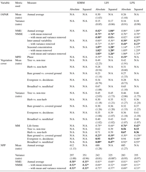
LPJ scores 0.82 and LPX scores 0.86 using NME for annual average fAPAR (Table 5). This difference in score is equiv-alent to a negligible (i.e.<5 %) change in the match to the observations. Both values are considerably better than val-ues for the mean of the data (1.00) and random resampling (1.19±0.004), with the match to observations being 15 % closer and 30 % closer respectively. The models also perform well for seasonal timing (Fig. 4), with scores of 0.19 (LPJ) and 0.18 (LPX) or the equivalent of an average of 34 days different from observations. For comparison, the seasonal timing of the mean of the data and random resampling is ca. 3 months different from observations. The models also perform well for inter-annual variability: LPJ scores 0.60 and LPX scores 0.50 using NME for inter-annual variability, compared to a mean score of 1.00 and a score of 1.21±0.34 from random resampling. The DGVM scores represent, re-spectively, a 40 % and 50 % better match to observations than the mean of the data. LPJ scores 1.07 and LPX scores 1.14 using NME for seasonal concentration, compared to 1.00 for the mean and 1.41±0.006 for random resampling. This means that the seasonal concentration of fapar in the DGVMs is, respectively, 7 % and 14 % worse than the mean of the data compared to observations.

3.1.2 Vegetation cover

LPJ scores 0.78 and LPX scores 0.76 using the MM for the prediction of life forms (Table 5), again a negligible dif-ference in performance (<3 %) compared to observations. Both values are better than obtained for the mean of the data (0.93) or by randomly resampling (0.88±0.002). Both mod-els were also better than mean and randomly resampling for bare ground. However, both models overestimate tree cover and underestimate herb cover by around a factor of 2 (Ta-ble 5). The scores for tree cover (LPJ: 0.62, LPX: 0.56) show, respectively, a 38 % and 24 % poorer match to ob-servations than the mean of the data (0.45), and a 15 % and 4 % poorer match to observations than randomly resampling (0.54±0.002). In the same way, the two DGVMs show a 40 % poorer match to observed grass cover than the mean of the data and a 6 % poorer match than randomly resampling. Both models are worse than mean and random resampling for phenology (Table 5).

3.1.3 NPP/GPP

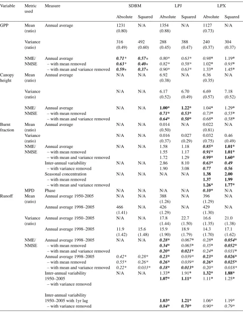
The models have NME scores for NPP of 0.58 (SDBM), 0.83 (LPJ) and 0.81 (LPX) (Table 5) – better than values obtained for the mean of the data (1.00) and random resam-pling (1.35±0.09). Removing the biases in mean and vari-ance (Table 5) improves the performvari-ance of all three models. The SDBM simulates 1.13 times higher NPP than observed, but correctly predicts the spatial variability shown by the ob-servations, whereas the two DGVMs overestimate NPP but underestimate the spatial variance in NPP. As a result, remov-ing the biases in the mean produces a much larger improve-ment in the DGVMs. In LPJ, for example, the score goes from 0.83 to 0.69, equivalent to a 29 % better match to the observations. The improvement in the SDBM is equivalent to only a 9 % better match to observations. The two DGVMs perform worse for GPP than NPP. LPX has an NME score of 0.81 for NPP but 0.98 for GPP – this is equivalent to a 17 % better match to NPP observations than to GPP observations. The SDBM performs better for GPP than the DGVMs, ob-taining an NME score of 0.71, which is better than the mean of the data (1.00) and randomly resampling (1.36±0.22).

3.1.4 Canopy height

LPJ scores 1.00 and LPX scores 1.04 using NME for the prediction of height (Table 5). These values lie between the mean (1.00) and random resampling (1.33±0.004) scores. This poor performance is due to modelled mean heights ca. 60–65 % lower than observed and muted variance (Ta-ble 5, Fig. 6). Removing the mean bias improves the score for both DGVMs to 0.71 for LPJ and 0.73 for LPX, equivalent to a 29 % and 30 % improvement in the match to observations. Model performance is further improved by removing bias in the variance, to 0.64 for LPJ (ca. 11 %) and 0.68 for LPX (ca. 6 %).

3.1.5 Burnt fraction

(12)

[image:12.595.50.548.123.701.2]

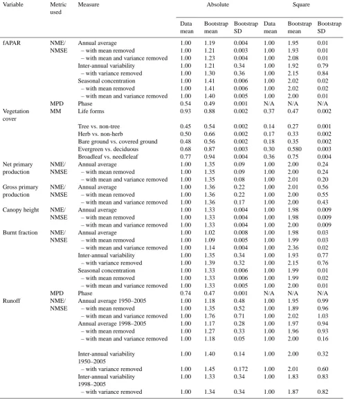
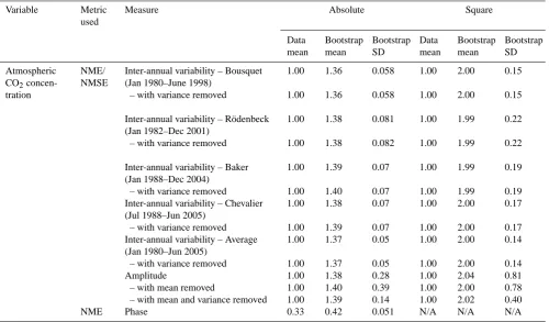
Table 4. Scores obtained using the mean of the data (Data mean), and the mean and standard deviation of the scores obtained from bootstrap-ping experiments (Bootstrap mean, Bootstrap SD). NME/NMSE denotes the normalised mean error/normalised mean squared error, MPD the mean phase difference and MM/SCD the Manhattan metric/squared chord distance metrics.

Variable Metric used

Measure Absolute Square

Data mean Bootstrap mean Bootstrap SD Data mean Bootstrap mean Bootstrap SD fAPAR NME/ NMSE Annual average – with mean removed

– with mean and variance removed

1.00 1.00 1.00 1.19 1.21 1.23 0.004 0.003 0.004 1.00 1.00 1.00 1.95 1.93 2.08 0.01 0.01 0.01 Inter-annual variability

– with variance removed

1.00 1.00 1.21 1.30 0.34 0.36 1.00 1.00 1.92 2.15 0.79 0.84 Seasonal concentration

– with mean removed

1.00 1.00 1.00 1.41 1.41 1.40 0.006 0.006 0.005 1.00 1.00 1.00 2.02 2.02 2.00 0.02 0.02 0.01

MPD Phase 0.54 0.49 0.001 N/A N/A N/A

Vegetation cover

MM Life forms 0.93 0.88 0.002 0.37 0.47 0.002

Tree vs. non-tree 0.45 0.54 0.002 0.14 0.27 0.001

Herb vs. non-herb 0.50 0.66 0.002 0.17 0.33 0.002

Bare ground vs. covered ground 0.48 0.56 0.002 0.18 0.35 0.002

Evergreen vs. deciduous 0.68 0.87 0.003 0.30 0.580 0.003

Broadleaf vs. needleleaf 0.77 0.94 0.004 0.36 0.75 0.004

Net primary production

NME/ NMSE

Annual average – with mean removed

1.00 1.00 1.00 1.35 1.35 1.35 0.09 0.09 0.08 1.00 1.00 1.00 2.00 2.00 2.01 0.24 0.24 0.20 Gross primary production NME/ NMSE Annual average – with mean removed

1.00 1.00 1.00 1.36 1.36 1.36 0.22 0.22 0.17 1.00 1.00 1.00 2.01 2.00 2.00 0.56 0.55 0.43 Canopy height NME/

NMSE

1.00 1.00 1.00 1.33 1.33 1.33 0.004 0.004 0.004 1.00 1.00 1.00 1.98 1.98 2.00 0.009 0.009 0.009 Burnt fraction NME/

NMSE

1.00 1.00 1.00 1.02 1.09 1.14 0.008 0.005 0.004 1.00 1.00 1.00 1.98 1.99 2.36 0.03 0.03 0.02 Inter-annual variability

1.00 1.00 1.35 1.39 0.34 0.32 1.00 1.00 1.93 2.15 0.77 0.76 Seasonal concentration

1.00 1.00 1.00 1.33 1.33 1.33 0.006 0.006 0.005 1.00 1.00 1.00 1.99 1.99 2.00 0.01 0.02 0.01

MPD Phase 0.74 0.47 0.001 N/A N/A N/A

Runoff NME/

NMSE

Annual average 1950–2005 – with mean removed

1.00 1.00 1.00 1.18 1.35 1.76 0.48 0.52 0.71 1.00 1.00 1.00 1.95 1.89 2.02 0.99 0.96 1.03 Annual average 1998–2005

1.00 1.00 1.00 1.17 1.27 1.18 0.28 0.33 0.05 1.00 1.00 1.00 1.97 1.96 2.00 0.94 0.93 0.16 Inter-annual variability 1950–2005

1.00 1.00 1.40 1.45 0.14 0.172 1.00 1.00 2.00 2.01 0.32 0.60 Inter-annual variability 1998–2005

(13)

[image:13.595.49.550.80.373.2]

Table 4. Continued.

Measure Absolute Square

Data mean

Bootstrap mean

Bootstrap SD

Data mean

Bootstrap mean

Bootstrap SD

Atmospheric CO2

concen-tration

NME/ NMSE

Inter-annual variability – Bousquet (Jan 1980–June 1998)

1.00

1.36

0.058

1.00

2.00

0.15

Inter-annual variability – R¨odenbeck (Jan 1982–Dec 2001)

1.00

1.38

0.081

0.082

1.00

1.99

0.22

Inter-annual variability – Baker (Jan 1988–Dec 2004)

1.00

1.39

1.40

0.07

1.00

1.99

0.19

0.19 Inter-annual variability – Chevalier

(Jul 1988–Jun 2005) – with variance removed

1.00

1.38

1.39

0.07

1.00

2.00

0.17

0.17 Inter-annual variability – Average

(Jan 1980–Jun 2005) – with variance removed

1.00

1.37

0.05

1.00

2.00

0.14

0.14 Amplitude

1.00 1.00 1.00

1.38 1.40 1.39

0.28 0.39 0.14

1.00 1.00 1.00

2.04 2.00 2.02

0.81 0.78 0.40

NME Phase 0.33 0.42 0.051 N/A N/A N/A

3.1.6 River discharge

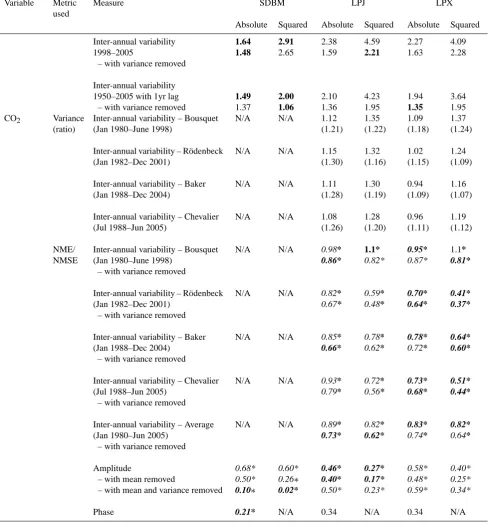
Comparing average runoff for 1950–2005, both DGVMs score 0.28 for NME, better than the mean (1.00) and ran-dom resampling (1.18±0.48). The models perform much less well for inter-annual comparisons, with NME scores of 1.33 (LPJ) and 1.32 (LPX), worse than 1.00 for the mean and 1.45±0.17 for random resampling. Agreement is slightly improved by removing variance bias (LPJ: 1.07, LPX: 1.11). Neither of the DGVMs examined here treat water-routing ex-plicitly. Introducing a one-year lag for inter-annual compar-isons (Fig. 8) produces a 21 % (LPJ) and 19 % (LPX) im-provement in the match to observations, confirming that tak-ing account of delays in water transport is important when assessing the inter-annual variation in runoff. All three mod-els were compared for 1998–2005. For annual average com-parisons, they all performed better than the mean and random resampling (Table 5). However, all models performed poorly for inter-annual variability, obtaining similar scores (1.64 to 2.38) compared to the mean (1.00) and random resampling (1.34±0.34). Removing variability bias and introducing a one-year lag improved performance, with the SDBM scoring 1.37, LPJ 1.36 and LPX 1.35.

3.1.7 CO2concentration

The generalised form of the seasonal cycle in CO2

concen-trations at different sites can be compared for all three mod-els. The SDBM scores 0.21 whereas LPJ scores 0.34 and LPX 0.34 in the MPD comparisons of seasonal timing, com-pared to the mean of the data (0.33) and random resam-pling (0.42±0.051). Thus, the SDBM produces an estimate of peak timing that is 22 days closer to observations than the mean of the data, while the DGVMs produce estimates that are 6 days further away from the observations than the mean of the data (Fig. 3). The scores for NME comparison of seasonal concentration for the SDBM (0.68), LPJ (0.46) and LPX (0.58) are all better than the mean (1.00) and ran-dom resampling (1.38±0.28). Thus, although the difference between the models is non-trivial (ca. 30 %), all three models are ca. 30–50 % closer to observations than the mean of the data. Only the DGVMs can be evaluated with respect to inter-annual variability in global CO2concentrations. Both models

(14)

[image:14.595.56.545.147.723.2]

Table 5. Comparison metric scores for model simulations against observations. Mean and variance rows show mean and variance of simula-tion for annual average values, followed in brackets by the ratio of the mean/variance with observed mean or variance in Table 3. Numbers in bold indicate the model with the best performance for that variable. Italic indicates model scores better than the mean of the data score listed in Table 4. Asterisks indicate model scores that are significantly better than randomly resampling listed in Table 4. NME/NMSE denotes the normalised mean error/normalised mean squared error, MPD the mean phase difference and MM/SCD the Manhattan metric/squared chord distance metrics. fAPAR is the fraction of absorbed photosynthetically active radiation, NPP net primary productivity, and GPP gross primary productivity.

Measure SDBM LPJ LPX

Absolute Squared Absolute Squared Absolute Squared

fAPAR Mean

(ratio)

Annual average N/A N/A 0.30

(1.63) N/A 0.26 (1.44) N/A Variance (ratio)

N/A N/A 0.15

(0.85) 0.17 (0.86) 0.16 (0.91) 0.18 (0.90) NME/ NMSE Annual average – with mean removed

N/A N/A 0.82* 0.75* 0.80* 1.04* 0.76* 0.83∗ 0.86* 0.76* 0.82* 1.09* 0.78* 0.90* Inter-annual variability – with variance removed

N/A N/A 0.60*

0.73* 0.36* 0.36* 0.50* 0.44* 0.27* 0.23* Seasonal concentration

N/A N/A 1.07*

1.02* 1.03* 1.28* 1.20* 1.26* 1.14* 1.05* 1.06* 1.37* 1.25* 1.31*

MPD Phase N/A N/A 0.19* N/A 0.18* N/A

Vegetation cover

Mean (ratio)

Tree vs. non-tree N/A N/A 0.49

(2.23)

N/A 0.42

(1.91)

N/A

Herb vs. non-herb N/A N/A 0.28

(0.54)

N/A 0.31

(0.60)

N/A

Bare ground vs. covered ground N/A N/A 0.23 (1.14)

N/A 0.27

(1.33)

N/A

Evergreen vs. deciduous N/A N/A 0.34

(0.79)

N/A 0.28

(0.73)

N/A

Broadleaf vs. needleleaf N/A N/A 0.67

Tree vs. non-tree N/A N/A 0.45

(2.03) 0.45 (1.73) 0.46 (2.06) 0.46 (1.75)

Herb vs. non-herb N/A N/A 0.30

(1.18) 0.35 (1.21) 0.32 (1.27) 0.36 (1.24) Bare ground vs. covered ground N/A N/A 0.30

(1.26) 0.36 (1.20) 0.32 (1.33) 0.37 (1.23)

Evergreen vs. deciduous N/A N/A 0.35

(1.06) 0.39 (1.07) 0.36 (1.18) 0.41 (1.18)

Broadleaf vs. needleleaf N/A N/A 0.40

(1.02) 0.43 (1.02) 0.43 (1.07) 0.46 (1.07)

MM Life forms N/A N/A 0.78* 0.44* 0.76* 0.42*

Tree vs. non-tree N/A N/A 0.62 0.39 0.56 0.33

Herb vs. non-herb N/A N/A 0.71 0.39 0.67 0.36

Bare ground vs. covered ground N/A N/A 0.23* 0.10* 0.30* 0.156*

Evergreen vs. deciduous N/A N/A 0.93 0.47* 0.94 0.48*

Broadleaf vs. needleleaf N/A N/A 0.89* 0.47* 0.92* 0.55*

NPP Mean

(ratio)

Annual average 612

(1.13) N/A 688 (1.28) N/A 685 (1.27) N/A Variance (ratio) 297 (1.00) 351 (0.96) 242 (0.81) 325 (0.887) 283 (0.95) 355 (0.97) NME/ NMSE Annual average – with mean removed

(15)

[image:15.595.58.542.87.708.2]

GPP Mean

(ratio)

Annual average 1231

(0.80) N/A 1354 (0.88) N/A 1127 (0.73) N/A Variance (ratio) 316 (0.49) 492 (0.60) 288 (0.45) 388 (0.47) 240 (0.37) 304 (0.37) NME/ NMSE Annual average – with mean removed

– with mean and variance removed 0.71* 0.63* 0.59∗ 0.57∗ 0.40∗ 0.37∗ 0.80* 0.82* 0.90* 0.63* 0.58* 0.63* 0.98* 1.02* 1.33* 1.19* 0.93* 1.45* Canopy height Mean (ratio)

N/A N/A 6.17

N/A N/A 1.00*

0.71* 0.64* 1.22* 0.53* 0.50* 1.04* 0.73* 0.68* 1.29* 0.55* 0.58* Burnt fraction Mean (ratio)

N/A N/A 0.016

N/A N/A 1.58

1.55 1.72 1.18 1.17 1.29 0.85* 0.91* 0.99* 1.01* 1.01* 1.60* Inter-annual variability

N/A N/A 2.86

1.90 8.10 3.08 0.63* 0.77 0.49 0.56 Seasonal concentration

N/A N/A N/A N/A 1.38

1.37 1.26*

2.00 1.99 1.77*

MPD Phase N/A N/A N/A N/A 0.10* N/A

Runoff Mean

(ratio)

Annual average 1950-2005 N/A N/A 388

(1.26)

N/A 396

(1.29)

N/A

Annual average 1998–2005 466 (1.41) N/A 426 (1.29) N/A 429 (1.30) N/A Variance (ratio)

Annual average 1950–2005 N/A N/A 17.8

(1.44) 22.7 (1.50) 16.6 (1.35) 21.0 (1.38) Annual average 1998–2005 11.9

(1.42) 15.6 (1.48) 15.9 (1.90) 18.9 (1.79) 14.3 (1.70) 17.1 (1.62) NME/ NMSE

N/A N/A 0.28* 0.34* 0.20* 0.067* 0.065* 0.021* 0.28* 0.35* 0.24* 0.054* 0.052* 0.031*

0.42* 0.55* 0.22* 0.28* 0.26* 0.033* 0.23* 0.26* 0.18* 0.039* 0.039* 0.013* 0.23* 0.26* 0.20* 0.026* 0.025* 0.018* Inter-annual variability 1950–2005

Inter-annual variability 1950–2005 with 1yr lag

N/A N/A 1.33*

(16)

[image:16.595.54.544.86.614.2]

Inter-annual variability 1998–2005

Inter-annual variability 1950–2005 with 1yr lag

1.64 1.48 1.49 1.37 2.91 2.65 2.00 1.06 2.38 1.59 2.10 1.36 4.59 2.21 4.23 1.95 2.27 1.63 1.94 1.35 4.09 2.28 3.64 1.95 CO2 Variance

(ratio)

N/A N/A 1.12

(1.21) 1.35 (1.22) 1.09 (1.18) 1.37 (1.24)

N/A N/A 1.15

(1.30) 1.32 (1.16) 1.02 (1.15) 1.24 (1.09)

N/A N/A 1.11

(1.28) 1.30 (1.19) 0.94 (1.09) 1.16 (1.07)

Inter-annual variability – Chevalier (Jul 1988–Jun 2005)

N/A N/A 1.08

(1.26) 1.28 (1.20) 0.96 (1.11) 1.19 (1.12) NME/ NMSE

N/A N/A 0.98*

0.86* 1.1* 0.82* 0.95* 0.87* 1.1* 0.81*

N/A N/A 0.82*

0.67* 0.59* 0.48* 0.70* 0.64* 0.41* 0.37*

N/A N/A 0.85*

0.66* 0.78* 0.62* 0.78* 0.72* 0.64* 0.60*

Inter-annual variability – Chevalier (Jul 1988–Jun 2005)

N/A N/A 0.93*

0.79* 0.72* 0.56* 0.73* 0.68* 0.51* 0.44*

Inter-annual variability – Average (Jan 1980–Jun 2005)

N/A N/A 0.89*

0.73* 0.82* 0.62* 0.83* 0.74* 0.82* 0.64* Amplitude

0.68* 0.50* 0.10∗ 0.60* 0.26∗ 0.02* 0.46* 0.40* 0.50* 0.27* 0.17* 0.23* 0.58* 0.48* 0.59* 0.40* 0.25* 0.34*

Phase 0.21* N/A 0.34 N/A 0.34 N/A

3.2 Sensitivity tests

3.2.1 Incorporating data uncertainties

In calculating the performance metrics, we have disregarded observational uncertainty. Few land-based datasets provide quantitative information on the uncertainties associated with

(17)

[image:17.595.105.495.65.411.2]

Fig. 4. Comparison of observed and simulated seasonal phase and seasonal concentration of fraction of absorbed photosynthetically active radiation (fAPAR) averaged over the period 1998–2005 from (a) seasonal phase from SeaWiFS (Gobron et al., 2006) and as simulated by (b) LPJ and (c) LPX; seasonal concentration from (d) SeaWiFS, (e) LPJ and (f) LPX. Hashed area in (a) and (d) shows areas where no comparison is possible.

values at each site or grid cell to calculate the maximum and minimum potential distance between models and observa-tions.

In the standard NME comparison for annual fractional burnt area, LPJ scores 1.58 while LPX scores 0.85. Taking into account the uncertainties produces minimum and maxi-mum scores of 1.27 and 1.85 for LPJ, and 0.35 and 1.17 for LPX. Since these ranges are non-overlapping, the improve-ment in the match to observations shown by LPX compared to LPJ is demonstrably larger than observational uncertainty. This is not the case for the Luyssaert et al. (2007) only site-based annual average NPP comparisons, where the ranges are 0.26–1.36 (SDBM), 0.37–1.43 (LPJ) and 0.39–1.50 (LPX). Similarly, the apparent biases in mean annual NPP shown by all three models are within the observational uncertainty. Re-moving the slight high bias in mean annual NPP produced an improvement in the performance of the SDBM, with a change in the Luyssaert et al. (2007) only score from 0.72 to 0.59, equivalent to a 18 % better match to the observations.

However, the range of scores obtained for the SDBM taking into account the observational uncertainties after removing the high bias is 0.21–1.25. As this overlaps with the scores obtained prior to removing these biases (0.26–1.36), the im-provement gained from removing the influence of the mean in NPP in the SDBM is less than the observational uncer-tainty.

Another approach to estimating the influence of uncer-tainty is to use alternative realizations of the observations. This approach has been used by the climate-modelling com-munity to evaluate performance against modern climate ob-servations (e.g. Gleckler et al., 2008) and is used here for CO2inter-annual comparisons. The scores obtained in

(18)

[image:18.595.52.285.62.421.2]

Fig. 5. Comparisons of observed and simulated NPP and GPP in kg C m−2. The NPP observations (x-axis) are from the dataset made by combining sites from the Luyssaert et al. (2007) dataset and the Ecosystem/Model Data Intercomparison dataset (Olson et al., 2001). The GPP observations are derived from the Luyssaert et al. (2007) dataset. The simulated values (y-axis) are annual aver-ages for the period 1998–2005. The observations are compared with NPP (a) and GPP (b) from the Simple Diagnostic Biosphere Model (SDBM), NPP (c) and GPP (d) from LPJ and NPP (e) and GPP (f) from LPX. The solid line shows the 1 : 1 relationship.

3.2.2 The influence of choice of dataset

The use of alternative datasets for a given variable implies that there are no grounds for distinguishing which is more reliable. It also highlights the fact that there is an element of subjectivity in the choice of datasets and that this introduces another source of uncertainty into the process of benchmark-ing. We have explicitly excluded from the benchmarking pro-cedure any datasets that involve manipulations of original measurements based on statistical or physical models that are driven by the same inputs as the vegetation models be-ing tested (e.g. MODIS NPP, remotely sensed evapotranspi-ration, upscaled GPP). However, such products often provide

Table 6. Mean annual gross primary production (GPP) normalised mean error (NME) comparison metrics using Luyssaert et al. (2007) and Beer et al. (2010) as alternative benchmarks. In the case of Beer et al. (2010), the comparisons are made for all grid cells (global) and also from the grid cells which contain sites in the Luyssaert et al. (2007) dataset (at sites).

Variable Measure SDBM LPJ LPX

GPP from global N/A N/A N/A

Luyssaert et al. (2007) at sites 0.71 0.80 0.98

GPP from global 0.56 0.60 0.51

Beer et al. (2010) at sites 0.34 0.84 0.74

global coverage of variables that may not be as well repre-sented in other datasets and thus could provide a useful alter-native realization of the observations.

Here, we test the use of the Beer et al. (2010) dataset as an alternative to the Luyssaert et al. (2007) GPP dataset. The Beer et al. (2010) GPP dataset is based on a much larger number of flux-tower measurements than are included in the Luyssaert et al. (2007) dataset, but uses both diagnostic mod-els and statistical relationships with climate to scale up these measurements to provide global coverage. We compare the annual average GPP scores using Beer et al. (2010), calcu-lated using all grid cells and considering only those grid cells which correspond to locations with site data in the Luyssaert et al. (2007) dataset. These comparisons (Table 6) show that LPX and SDBM perform better against the Beer et al. (2010) dataset than against the Luyssaert et al. (2007) at the site lo-cations, while the results obtained for LPJ against the two datasets are roughly similar. There is a further improvement in performance when the models are compared against all the grid cells. The improvement in performance at the site loca-tions presumably reflects the fact that the Beer et al. (2010) dataset smooths out idiosyncratic site characteristics; the ad-ditional improvement in performance in the global compari-son reflects both the smoothing and the much larger number of flux sites included in the Beer et al. (2010) dataset. Never-theless, the conclusion that the SDBM performs better than the DGVMs is not influenced by the choice of dataset. LPJ performs marginally better than LPX when the Luyssaert et al. (2007) dataset is used as the benchmark (0.8 versus 0.98), but worse than LPX when the Beer et al. (2010) dataset is used as a benchmark (0.6 versus 0.51). This indicates that the difference between the two DGVMs is less than the ob-servational uncertainty.

[image:18.595.312.544.137.211.2]

(19)

[image:19.595.99.499.61.296.2]

Fig. 6. Comparisons of observed and simulated height. (a) Observed canopy height (in 2005) from the Simard et al. (2011) dataset compared to (b) simulated height in the same year from LPX; (c) LPX-simulated height, multiplied by a factor of 2.67 so that the simulated global mean height is the same as the observations; (d) height from (c) with values reduced by a factor of 1.40 about the mean so that the simulations have the same global mean and variance as the observations.

the annual average burnt fraction changes from 1.58 (against GFED3) to 1.91 (against GFED2) for LPJ and from 0.85 (GFED3) to 0.92 (GFED2) for LPX (i.e. both models pro-duce a better match to GFED3 than to GFED2), but the dif-ference between the two models is preserved (i.e. LPX, with its more explicitly process-based fire model, is more realistic than LPJ).

3.2.3 Benchmarking the sensitivity to parameter tuning

Benchmarking can be used to evaluate how much tuning of individual parameters improves model performance and to ensure that the simulations capture specific processes cor-rectly. We examine how well the current system serves in this respect by running sensitivity experiments using the SDBM. The SDBM underestimates the amplitude of CO2 seasonal cycle (Fig. 3). A better match to CO2 observations can be

achieved by tuning the light-use efficiency parameter (ε in Eq. 12). The best possible match to CO2 seasonal ampli-tude (0.18) is obtained whenεis equal to 1.73 g C MJ−1_{, but}

this increases both the mean and the variance of NPP com-pared to observations: the overall performance of the SDBM is therefore worse (Table 7). The seasonal amplitude of CO2

depends on simulating the correct balance between NPP and

Rh. Thus, given that the model produces a reasonable

simula-tion of annual average NPP, improvement in CO2seasonality

should come from changes in the simulation ofRh.

Remov-ing the requirement that NPP andRhare in equilibrium, by

setting total NPP to be 1.2 timesRh, improves the CO2

sea-sonal amplitude score to 0.51. In the baseline simulation, the

Q10 for Rh is 1.5 (Eq. 13). Changing this response by

in-creasing Q10 to 2 degrades the simulation of the seasonal

amplitude and phase of CO2, while decreasing Q10 to 1.3

improves the simulation of the seasonal amplitude and phase of CO2(Table 7). Removing the seasonal response ofRhto

moisture (i.e. removingαfrom Eq. 13) improves the score for seasonal amplitude (0.39) but does not change the score for the phase. However, this degrades its performance against annual average NPP from 0.58 to 0.82. We expect thatRh

should be sensitive to soil moisture changes, but this analysis suggests that the treatment of this dependency in the SDBM is unrealistic.

4 Discussion and conclusion

Model benchmarking serves multiple functions, including (a) showing whether processes are represented correctly in a model, (b) discriminating between models and determining which performs better for a specific process, and (c) compar-ing between the model scores and those obtained by com-paring mean and random resampling of observations, thus helping to identify processes that need improvement.

As found by Heimann et al. (1998), the SDBM produces a good simulation of the seasonal cycle of atmospheric CO2