SUPERPIXEL SEGMENTATION BASED AUTOMATIC
CLOUD DETECTION
*MISS K.JEYA, **MRS C.VINOLA, ***DR.D.C.JOY WINNIE WISE
*ME-CSE, Francis Xavier engineering college, Tirunelveli, India
**Assistant Professor CSE Department, Francis Xavier engineering college, Tirunelveli, India ***M.E.,Ph.D
ABSTRACT
INTRODUCTION
Digital image processing is the use of computer algorithms to perform image processing on digital images. As a subcategory or field of digital signal processing, digital image processing has many advantages over analog image processing. It allows a much wider range of algorithms to be applied to the input data and can avoid problems such as the build-up of noise and signal distortion during processing. Since images are defined over two dimensions (perhaps more) digital image processing may be modeled in the form of multidimensional systems. Clouds play an important role in hydrological cycle and affect the energy balance on local and global scopes via interacting with solar and terrestrial radiation. Most cloud related research requires ground-based cloud observation, such as cloud cover. At present, cloud cover is still estimated by human observers at meteorological observation stations. However, this method takes high cost in terms of human resources, and the results obtained from different observers are often inconsistent. Thus, automatic estimation techniques for cloud cover are eagerly required in this field. To achieve this goal, some instruments for capturing ground-based clouds, such as whole sky imager, total sky imager and infrared cloud analyzer have been developed. Those instruments could obtain
continuous all-sky images with a set time interval. Moreover, a lot of algorithms are proposed to estimate the cloud cover based on these captured all-sky images. Cloud detection, which classifies each pixel of all-sky images into cloud or clear sky element, is needful for cloud cover estimation. Currently, most cloud detection algorithms treat color as the primary characteristic for distinguishing cloud from clear sky. This is due to the scattering difference between cloud particles and air molecules. More specifically, cloud particles scatter similar blue (B) and red (R) intensity, whereas clear sky scatters more B than R intensity. Based on this, Long et al. propose a threshold algorithm for cloud detection according to a certain radio of R over B intensity using red green- blue (RGB) image. Specifically, pixels with R/B greater than 0.6 are identified as cloud, otherwise as clear sky. Kreuter et al. report a different threshold of 1.3 on the B/R radio for identifying cloud, which is illustrated to be a more suitable choice than the previously mentioned value of 0.6.
RELATED WORK
Nobuyuki otsu [1] has proposed a nonparametric and unsupervised method of automatic threshold selection for picture segmentation is presented. An optimal threshold is selected by the discriminant criterion, namely, so as to maximize the separability of the resultant classes in gray levels. Qingyong Li [2] has proposed thin cloud detection for all-sky images is a challenge in ground-based sky-imaging systems because of low contrast and vague boundaries between cloud and sky regions. . In this model, each pixel is represented by a combined-feature vector that aims at improving the disparity between thin cloud and sky. The distribution of each label in the feature space is defined as a Gaussian model. J. Yang et al [3] has proposed an automatic cloud detection algorithm, “green channel background subtraction adaptive threshold” (GB SAT), which incorporates channel selection, background simulation, computation of solar mask and cloud mask, subtraction, adaptive threshold, and binarization. Several experimental cases show that the GBSAT algorithm is robust for all types of test total sky images and has more complete and accurate retrievals of visual effects than those found through traditional methods. Sylvio Luiz [4] has describes the use of multidimensional Euclidean geometric distance (EGD) and Bayesian methods to characterize and classify the sky and cloud patterns present in image pixels. From specific images and using visualization tools, it was noticed that sky and cloud patterns occupy a typical locus on the red–green–blue (RGB) color space. Genkova [5] has takes theeffort to resolve uncertainties about global climate change, the Atmospheric Radiation Measurement (ARM) Program (www.arm.gov) is improving the treatment of cloud radiative forcing and feedbacks in general circulation models. Understanding cloud properties and how to predict them is critical because cloud properties may very well change as climate changes. The amount of clouds and cloud spatial and vertical distribution at any given time are required input parameter for improving the performance of general circulation models.
image, which acts as a kind of clustering algorithm. As the SPS based on the characteristics of the image, such as contour and texture, the pixels in each super pixel could guarantee the consistency most of the time, i.e., the pixels in each super pixel will belong to the same group (cloud or clear sky) as much as possible. Then, we further detect cloud based on these superpixels. 1) SPS: SPS divides an image to a series of irregular blocks according to texture similarity, brightness similarity, and contour continuity. For a ground-based cloud image, the segmentation can be treated as a graph partitioning problem. The nodes of the graph are the entities that we want to partition, and here, they are the pixels; the edges between two nodes correspond to the similarity with which these two nodes belong to one group. Let G={V, E} be a weighted undirected graph, where V denotes the nodes and E denotes the edges; the segmentation can be formulated by the following objective function:
y = arg min Ncut = arg (1)
where W = {wij} is the association matrix and wij is the weight between nodes i and j in the graph.
D is the diagonal matrix, where Dii = , i.e., Dii is the sum of the weights of all of the
connections to node i. y = {a, b}N is a binary indicator vector specifying the group identity for each pixel, i.e., yi = a if pixel i belongs to group A, and yi = b if pixel I belongs to group B. Here,
A (or B) is a partition of the graph nodes; combining A and B is the set of all nodes. N is the number of pixels. From the objective function of SPS (1), we know that the segmentation fundamentally depends on the weights (wij), which should be large for pixels from the same group,
while small otherwise. Since contour and texture are the main characteristics of clouds, the weight is defined as the product of the contour and texture cues [13], i.e., wij = . denotes
contour cue, which is adopted from the intervening contour method; denotes texture cue, which is computed by χ2 test. Normalized cut algorithm is applied to solve (4.1). After applying the SPS algorithm, it can be seen that each cloud image can be adaptively divided into a series of superpixels according to the characteristics of clouds, as shown in Fig. 4.1(c). In most situations, the pixels maintain a high degree of consistency in each super pixel, i.e., they belong to cloud or clear sky elements.
CLOUD DETECTION SCHEME
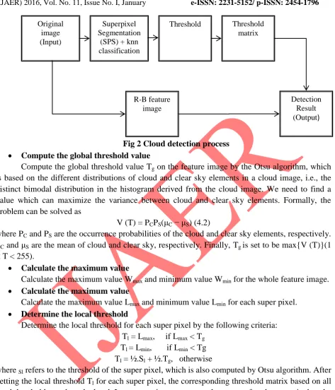
Fig 2 Cloud detection process
Compute the global threshold value
Compute the global threshold value Tg on the feature image by the Otsu algorithm, which
is based on the different distributions of cloud and clear sky elements in a cloud image, i.e., the distinct bimodal distribution in the histogram derived from the cloud image. We need to find a value which can maximize the variance between cloud and clear sky elements. Formally, the problem can be solved as
V (T) = PCPS(μC − μS) (4.2)
where PC and PS are the occurrence probabilities of the cloud and clear sky elements, respectively.
μC and μS are the mean of cloud and clear sky, respectively. Finally, Tg is set to be max{V (T)}(1
< T < 255).
Calculate the maximum value
Calculate the maximum value Wmax and minimum value Wmin for the whole feature image. Calculate the maximum value
Calculate the maximum value Lmax and minimum value Lmin for each super pixel. Determine the local threshold
Determine the local threshold for each super pixel by the following criteria: Tl = Lmax, if Lmax < Tg
Tl = Lmin, if Lmin < Tg
Tl = ½.Sl + ½.Tg, otherwise
where Sl refers to the threshold of the super pixel, which is also computed by Otsu algorithm. After
getting the local threshold Tl for each super pixel, the corresponding threshold matrix based on all
local thresholds can be calculated. In our experiment, we treat the center of each super pixel as the location of local threshold. Based on this, a threshold matrix with the same size as the R-B feature image is obtained by bilinear interpolation. Based on the threshold matrix, we can implement cloud detection in the cloud image. In particular, we compute the difference between the threshold matrix and feature image pixel by pixel. If the result is greater than 0, the corresponding pixel is classified as a cloud element, otherwise as a clear sky one. Fig. 4.2 shows an example for the
1) Our SPS can adapt with the diverse shape, size, and location of clouds and can adaptively divide the image into a series of irregular regions.
2) R-B as feature image is used, which can increase the differences of cloud and clear sky elements.
3) For each super pixel, its local threshold value is calculated, which is suitable for all kinds of cloud images, especially when cloud and clear sky pixels exist in the same super pixel simultaneously.
4) The threshold matrix is calculated by bilinear interpolation, which can guarantee the smoothness of thresholds between different superpixels and avoid the boundary effect in cloud detection. Correspondingly, better detection results should be achieved.
4.3.5 Classification using KNN classifier
Classification using an instance-based classifier can be a simple matter of locating the nearest neighbour in instance space and labelling the unknown instance with the same class label as that of the located (known) neighbour. This approach is often referred to as a nearest neighbour classifier. The downside of this simple approach is the lack of robustness that characterize the resulting classifiers. The high degree of local sensitivity makes nearest neighbour classifiers highly susceptible to noise in the training data. More robust models can be achieved by locating k, where k > 1, neighbours and letting the majority vote decide the outcome of the class labelling. A higher value of k results in a smoother, less locally sensitive, function. The nearest neighbor classifier can be regarded as a special case of the more general k-nearest neighbours classifier, hereafter referred to as a kNN classifier. The drawback of increasing the value of k is of course that as k approaches n, where n is the size of the instance base, the performance of the classifier will approach that of the most straightforward statistical baseline, the assumption that all unknown instances belong to the class most frequently represented in the training data.
This problem can be avoided by limiting the influence of distant instances. One way of doing so is to assign a weight to each vote, where the weight is a function of the distance between the unknown and the known instance. By letting each weight be defined by the inversed squared distance between the known and unknown instances votes cast by distant instances will have very little influence on the decision process compared to instances in the near neighbourhood. Distance weighted voting usually serves as a good middle ground as far as local sensitivity is concerned. Seven different sky conditions are distinguished: high thin clouds, high patched cumuliform clouds, stratocumulus clouds, low cumuliform clouds, thick clouds, strati form clouds and clear sky.
SIMULATION RESULTS
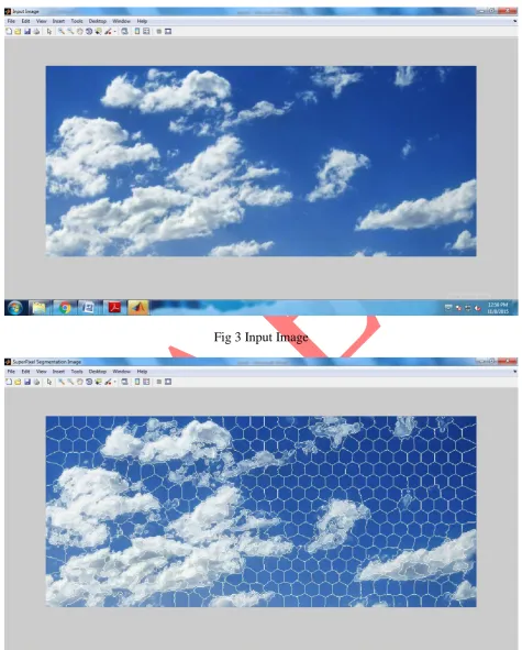
Fig 3 Input Image
Fig 4 shows the super pixel segmentation image. For each cluster in the image super pixels are calculated and their boundaries are drawn. In the above figure the super pixel are grouped and it is represented as white boundary.
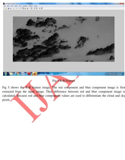
Fig 5 R-B Feature
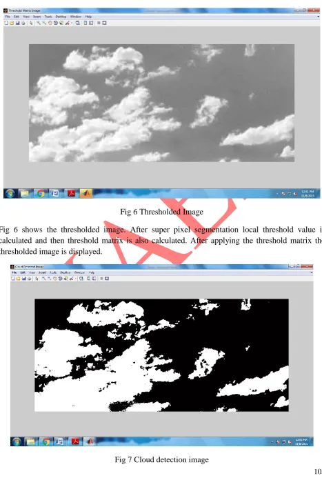
Fig 6 Thresholded Image
Fig 7 shows that the cloud detection image. In this image white color pixels represents cloud pixels and black color represents sky pixels. The final detected image is high patched cumuliform cloud.
CONCLUSION
In the project, an automatic cloud detection algorithm based on SPS is proposed. Compared with the fixed threshold, global threshold, and local threshold interpolation algorithms, the experimental results demonstrate that our algorithm achieves the highest performance for cloud detection. Also the algorithm seven different sky conditions are distinguished: high thin clouds, high patched cumuliform clouds, stratocumulus clouds, low cumuliform clouds, thick clouds, strati form clouds and clear sky.
REFERENCES
1. Nobuyuki Otsu “A Threshold Selection Method from Gray-Level Histograms” IEEE Transactions On Systrems, Man, and Cybernetics, Vol. Smc-9, No. 1, January 2000
2. Qingyong Li, Member, IEEE, Weitao Lu, Jun Yang, and James Z. Wang Thin Cloud Detection of All-Sky Images Using Markov Random Fields IEEE GEOSCIENCE AND REMOTE SENSING LETTERS, VOL. 9, NO. 3, MAY 2012
3. J. Yang, Q. Min, W. Lu, W. Yao, Y. Ma, J. Du, and T. Lu “An automated cloud detection method based on green channel of total sky visible images” Atmos. Meas. Tech. Discuss., 8, 4581–4605, 2015
4. SYLVIO LUIZ MANTELLI NETO “The Use of Euclidean Geometric Distance on RGB Color Space for the Classification of Sky and Cloud Patterns”, JOURNAL OF ATMOSPHERIC AND OCEANIC TECHNOLOGY VOLUME 27