Vol. 16, No. 2, 2018, 255-263
ISSN: 2279-087X (P), 2279-0888(online) Published on 1 February 2018
www.researchmathsci.org
DOI: http://dx.doi.org/10.22457/apam.v16n2a1
Annals of
One Modulo Three Root Square Mean Labeling of Some
Disconnected Graphs
M. Jaslin Melbha1 and C. Jayasekaran2
1
Department of Mathematics, Women’s Christian College
Nagercoil - 629001, TamilNadu, India. Email: [email protected]
2
Department of Mathematics, Pioneer Kumaraswamy College Nagercoil - 629003, TamilNadu, India. Email: [email protected]
Received 10 January 2018; accepted 28 January 2018
Abstract. A graph G is said to be one modulo three root square mean graph if there is an injective function φ from the vertex set of G to the set {0, 1, 3, …, 3q-2, 3q} where q is the number of edges of G and φ induces a bijection φ* from the edge set of G to{1, 4, …,
3q-2} given by φ*(uv) = or and the function φ is
called one modulo three root square mean labeling of G. The concept of one modulo three root square mean labeling was introduced by Jayasekaran and Jaslin Melbha and they investigated some graphs are one modulo three root square mean graphs. In this paper we prove that some disconnected graphs are one modulo three root square mean labeling.
Keywords: one modulo three root square mean labeling, one modulo three root square mean graphs.
AMS Mathematics Subject Classification (2010): 05C99, 05C22
1. Introduction
We begin with simple, finite, connected and undirected graph. For standard terminology and notations we follow Harary [1]. A graph labeling is an assignment of integers to the vertices or edges or both subject to certain condition(s). If the domain of the mapping is the set of vertices (edges) then the labeling is called a vertex labeling (an edge labeling). Several types of graph labeling and a detailed survey are available in [2]. A very good application of graph labeling is given in [3,4]
Jayasekaran and David Raj introduced the concept one modulo three harmonic mean labeling of graphs in [5]. Root square mean labeling was introduced by Sandhya, Somasundaram and Anusa in [6]. Jayasekaran and Jaslin Melbha introduced the concept one modulo three root square mean labeling of graphs in [7]. Further they investigated some graphs are one modulo three root square mean graphs [8]. Not every graph is one modulo three root square mean. For example, star graph K1, n, where n ≥ 4 is not a one
We will provide a brief summary of definitions and other information’s which are necessary for our present investigation.
Definition 1.1. A graph G is said to be one modulo three root square mean graph if there
is an injective function φ from the vertex set of G to the set {0, 1, 3, …, 3q-2, 3q} where q is the number of edges of G and φ induces a bijection φ* from the edge set of G to{1, 4,
…, 3q-2} given by φ*(uv) = or and the function φ is
called one modulo three root square mean labeling of G.
Definition 1.2. The corona of two graphs G1 and G2 is the graph G = G1ʘG2 formed from
one copy of G1 and || copies of G2 where ith vertex of G1 is adjacent to every
vertices in the ith copy of G2.
Definition 1.3. The graph PnʘK1 is called a comb.
Definition 1.4. The product P2×Pn is called a ladder and it is denoted by Ln. The ladder
graph Ln is a planar undirected graph with 2n vertices and 3n-2 edges.
Definition 1.5. The union of two graphs G1 = (V1, E1) and G2 = (V2, E2) is a graph G = G1∪G2 with vertex set V = V1∪V2 and the edge set E = E1∪E2.
Theorem 1.6. The ladder Ln is a one modulo three root square mean graph for n ≠ 2 [6].
Theorem 1.7. Pm ∪(PnʘK1) is a one modulo three root square meangraph [6].
2. Main results
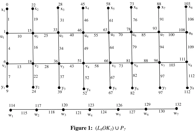
Theorem 2.1. (Lm ʘK1) ∪ Pn is one modulo three root square mean graph.
Proof: Let u1u2…um and v1v2 ...vm be two paths of length m. Join ui and vi, 1≤ i≤ m. The
resultant graph is Lm. For 1≤ i≤ m, let xi be the pendant vertex adjacent to ui and yi be the
pendant vertex adjacent to vi. Then we get the graph Lm ʘ K1. Let w1w2…wn be the path
Pn. Let G = (Lm ʘK1) ∪ Pn with V(G) ={ui, vi, xi, yi, wj /1≤ i≤ m, 1≤ j≤ n} and E(G) =
{uivi,uixi, viyi, vjvj+1, ujuj+1, wjwj+1/1≤i≤m, 1≤ j≤ n-1}. Then G has 4m+n vertices and
5m+n-3 edges. Define a function ϕ : V(G)→ {0, 1, 3,…, 3q-2, 3q} by ϕ(u1) = 1, ϕ(u2) =
15, ϕ(u3) = 33, ϕ(u4) = 46, ϕ(ui) = 15i-12, 5 ≤ i ≤ m; ϕ(x1) = 0, ϕ(x2) = 22, ϕ(x3) = 28,
ϕ(x4) = 45, ϕ(xi) = 15i-17, 5 ≤ i ≤ m; ϕ(v1) = 6, ϕ(v2) = 18, ϕ(v3) = 36, ϕ(vi) = 15i-9, 4 ≤ i
≤ m; ϕ(y1) = 9, ϕ(y2) = 24, ϕ(y3) = 39, ϕ(yi) = 15i-8, 4≤ i ≤m; ϕ(wi) = 15m+3i-9, 1≤ i ≤ n.
Then ϕ induces a bijection ϕ*: E(G) → {1, 4, …, 3q-2}, where ϕ*(uiui+1) = 15i-5, 1≤ i ≤
m-1; ϕ*(u1x1) = 1, ϕ*(u2x2) = 19, ϕ*(uixi) = 15i-14, 3 ≤ i ≤ m; ϕ*(u1v1) = 4, ϕ*(u2v2) = 16,
ϕ*(uivi) = 15i-11, 3 ≤ i ≤ m; ϕ*(v1y1) = 7, ϕ*(v2y2) = 22, ϕ*(viyi) = 15i-8, 3 ≤ i ≤ m;
ϕ*(vivi+1) = 15i-2, 1≤ i ≤ m-1; ϕ*(wiwi+1) = 15m+3i-8, 1≤ i ≤ n-1. Hence (Lm ʘK1) ∪ Pn is
one modulo three root square mean graph.
Figure 1: (L8ʘK1) ∪ P7
Theorem 2.3. (Lm ʘK1) ∪(PnʘK1) is one modulo three root square mean graph.
Proof: Let u1u2…um and v1v2 ...vm be two paths of length m. Join ui and vi, 1≤ i≤ m. The
resultant graph is Lm. For 1≤ i≤ m, let xi be the pendant vertex adjacent to ui and yi be the
pendant vertex adjacent to vi. Then we get the graph Lm ʘ K1. Let Pn be the path v1v2…vn.
Let wi be the vertex adjacent to vi, 1≤i≤n. The resultant graph is PnʘK1. Let G = (Lm
ʘK1) ∪(PnʘK1) with V(G) ={ui, vi, xi, yi, sj, tj /1≤ i≤ m, 1≤ j≤ n} and E(G) = {uivi,uixi,
viyi, vjvj+1, ujuj+1,sjtj, sjsj+1/1≤i≤m, 1≤ j≤ n-1}. Then G has 4m+2n vertices and 5m+2n-3
edges. Define a function ϕ : V(G)→ {0, 1, 3,…, 3q-2, 3q} by ϕ(u1) = 1, ϕ(u2) = 15, ϕ(u3) =
33, ϕ(u4) = 46, ϕ(ui) = 15i-12, 5 ≤ i≤ m; ϕ(x1)= 0, ϕ(x2)= 22, ϕ(x3)= 28, ϕ(x4)= 45, ϕ(xi)=
15i-17, 5 ≤ i≤ m; ϕ(v1)= 6, ϕ(v2) = 18, ϕ(v3) = 34, ϕ(vi) = 15i-9, 4 ≤ i≤ m; ϕ(y1) = 9, ϕ(y2)
= 24, ϕ(y3) = 39, ϕ(yi) = 15i-8, 4≤ i≤ m; ϕ(si) = 15m+6i-9 for all odd i ≤ n; ϕ(si)
=15m+6i-12 for all even i ≤ n; ϕ(ti) = 15m+6i-12 for all odd i ≤ n; ϕ(ti) = 15m+6i-9 for all even i ≤
n. Then ϕ induces a bijection ϕ*: E(G)→ {1, 4, …, 3q-2}, where ϕ*(uiui+1) = 15i-5, 1≤ i ≤
m-1; ϕ*(u1x1) = 1, ϕ*(u2x2) = 19, ϕ*(uixi) = 15i-14, 3 ≤ i ≤ m; ϕ*(u1v1) = 4, ϕ*(u2v2) = 16,
ϕ*(uivi) = 15i-11, 3 ≤ i ≤ m; ϕ*(v1y1) = 7, ϕ*(v2y2) = 22, ϕ*(viyi) = 15i-8, 3 ≤ i ≤ m;
ϕ*(vivi+1) = 15i-2, 1≤ i ≤ m-1; ϕ*(siti) = 15m+6i-11, 1≤ i ≤ n; ϕ*(sisi+1) = 15m+6i-8, 1≤ i ≤
n-1. Hence (Lm ʘK1) ∪(PnʘK1) is one modulo three root square mean graph.
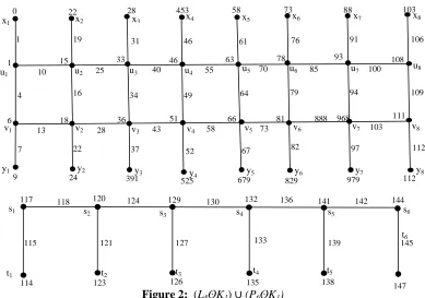
Example 2.4. A one modulo three root square mean labeling of (L8ʘK1) ∪ (P6ʘK1) is given in figure 2.
24 22 0 1 9 15 18 64 61 1 13 4 66 6 34 u1 v1 x1
v3 v4
v2
u2 u3 u4
x2 x3 x4
y1 y2 y3 y4
52 39
58
7 22
16 19 28 94 106 111 31 67 88 51 40 109 67 73 28
25 55
58 10 x5 u5 y5 76 93 82 45
x6 x7 x8
73 88 103
46 91
33 46 63 78 108
100 85
u6 u7 u8
70
49 79
36
43 v5 v6 v7 v8
81 96
103
37 52 97 112
82y6 97 112
y7 y8
132 130 129 127 126 124 123 121 120 117 114
115 118
Figure 2: (L8ʘK1) ∪ (P6ʘK1)
Theorem 2.5. Pn ∪Pm is a one modulo three root square mean graph.
Proof: Let u1u2…un be the path Pn and v1v2 ...vm be the path Pm. Let G = Pn ∪Pm with
V(G) = {ui, vj /1≤ i≤ n, 1≤ j≤ m} and E(G) = {uiui+1, vjvj+1 /1≤ i≤ n-1, 1≤ j≤ m-1}. Then
G has n+m vertices and n+m-2 edges. Define a function ϕ : V(G) → {0, 1, 3,…, 3q-2, 3q} by ϕ(u1) = 0, ϕ(u2) = 1, ϕ(ui) = 3(i-1), 3 ≤ i ≤ n-1, ϕ(un) = 3n-5; ϕ(vj) = 3n+3j-6, 1≤ j ≤
m-1, ϕ(vm) = 3n+3j-8. Then ϕ induces a bijection ϕ*: E(G) → {1, 4, …, 3q-2}, where
ϕ*(uiui+1) = 3i-2, 1≤ i ≤ n-1; ϕ*(vjvj+1) = 3n+3j-5, 1≤ j≤ m-1. Hence Pn ∪ Pm is a one
modulo three root square mean graph .
Example 2.6. A one modulo three root square mean labeling of P7 ∪ P6 is given in figure 3.
Figure 3: P7 ∪ P6
Theorem 2.7. Lm ∪ Pn is a one modulo three root square mean graph for m ≠ 2 and n ≠ 3.
t6 s1 t1 141 132 129 120 117 115
114 123 126 135 138
136 130
124 118
121 127 133 139
s2 s3 s4 s5
t2 t3 t4 t5
s6 144 145 147 142 16 16 15 13 12 10 9 7 6 1 0
1 4
u1 u2 u3 u4 u5 u6 u7
18 v1 31 31 30 28 27 25 24 21
19 v2 22 v3 v4 v5 v6
24 22 0 1 9 15 18 64 61 1 13 4 66 6 34 u1 v1 x1
v3 v4
v2
u2 u3 u4
x2 x3 x4
y1 y2 y3 y4
525 391
58
7 22
16 19 28 94 106 111 31 679 888 51 40 109 67 73 28
25 55
58 10 x5 u5 y5 76 93 82 453
x6 x7 x8
73 88 103
46 91
33 46 63 78 108
100 85
u6 u7 u8
70
49 79
36
43 v5 v6 v7 v8
81 968
103
37 52 97 112
829 y6 979 y7 112
Proof: Let u1u2…um and v1v2 ...vm be two paths of length m. Join ui and vi, 1≤ i≤ m. The
resultant graph is Lm. Let w1w2…wn be the path Pn. Let G = Lm ∪ Pn with V(G) = {ui, vi,
wj /1≤ i≤ m, 1≤ j≤ n} and E(G) = {uiui+1, vivi+1, uivi, unvn, wjwj+1/1≤ i≤ m-1, 1≤ j≤ n-1}.
Then G has 2m+n vertices and 3m+n-3 edges.
Case 1. m = 1
In this case, L1 ∪ Pn = P2 ∪ Pn. By Theorem 2.5 P2 ∪ Pn is a one modulo three root
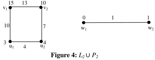
square mean graph. Case 2. = 2
Sub case 2.1. = 2
In this case, Lm ∪ Pn = L2 ∪ P2. Define a function ϕ : V(G) →{0, 1, 3, …, 3q-2, 3q} by
ϕ(u1) = 3, ϕ(u2) = 4, ϕ(v1) = 15, ϕ(v2) = 10, ϕ(w1) = 0, ϕ(w2) = 1. Then ϕ induces a
bijection ϕ*: E(G) → {1, 4, …, 3q-2}, where ϕ*(u1u2) = 4, ϕ*(u1v1) = 10, ϕ*(u2v2) = 7,
ϕ*(v1v2) =13, ϕ*(w1w2) =1. Thus the edges get distinct labels 1, 4, …, 13. In this case ϕ
is a one modulo three root square mean labeling for G. A one modulo three root square mean labeling of L2 ∪ P2 is given in figure 4.
Figure 4: L2 ∪ P2
Sub case 2.2. = 3
In this case, Lm ∪ Pn = L2 ∪ P3. It has 6 edges and 7 vertices. When we label these 7 vertices from the vertex set {0, 1, 3, …, 18}, atleast two edges get the same labels and hence L2 ∪ P3 is not one modulo three root square mean labeling.
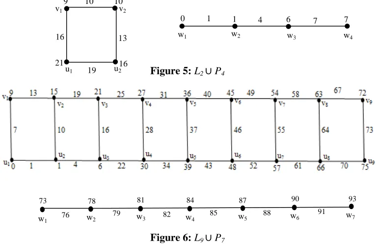
Sub case 2.3. ≥ 4
In this case, Lm ∪ Pn = L2 ∪ Pn. Define a function ϕ : V(G) →{0, 1, 3, …, 3q-2, 3q} by
ϕ(u1) = 3n+9, ϕ(u2) = 3n+4; ϕ(v1) = 3n-3, ϕ(v2) = 3n-2; ϕ(w1) = 0, ϕ(w2) = 1, ϕ(wi) =
3(i-1), 4 ≤ i ≤ n-1; ϕ(wn) = 3n-5. Then ϕ induces a bijection ϕ*: E(G) → {1, 4, …, 3q-2},
where ϕ*(u1u2) = 3n+7, ϕ*(u2v2) = 3n+1, ϕ*(u1v1) = 3n+4, ϕ*(v1v2) = 3n-2; ϕ*(wiwi+1)=
3i-2, 1≤ i≤ n-1. Thus the edges get distinct labels 1, 4, …, 3q-2. In this case ϕ is a one modulo three root square mean labeling for G.
Case 3. ≥ 3
Define a function ϕ : V(G) →{0, 1, 3, …, 3q-2, 3q} by ϕ(u1) = 0, ϕ(u2) = 1, ϕ(u3) = 6,
ϕ(ui) = 9i-6, 4≤ i≤ m; ϕ(vi) = 6i+3, 1≤ i≤ 3; ϕ(vi) = 9i-9, 4≤ i≤ m; ϕ(w1) = 9m-8, ϕ(wi) =
9(m-1)+3i, 2≤ i ≤ n. Then ϕ induces a bijection ϕ*: E(G) → {1, 4, …, 3q-2}, where
ϕ*(u1u2) = 1, ϕ*(u2u3)= 4, ϕ*(u3u4)= 22, ϕ*(uiui+1)= 9i-2, 4≤ i ≤ m-1; ϕ*(vivi+1)= 6i+7, 1≤
i ≤ 3; ϕ*(vivi+1)= 9i-5, 4≤ i≤ m-1; ϕ*(u1v1)= 7, ϕ*(u2v2) = 10, ϕ*(u3v3) =16, ϕ*(uivi) =
9i-8, 4≤ i≤ m; ϕ*(wiwi+1) = 9m+3i-8, 1≤ i≤ n-1. Thus the edges get distinct labels 1, 4, …, 4
10 15
3 4
7 13
10
0 1 1
u1 u2
v2
v1
3q-2. In this case ϕ is a one modulo three root square mean labeling for G. Hence Lm ∪Pn
is a one modulo three root square mean graph for 2 and n 3.
Example 2.8. A one modulo three root square mean labeling of L2 ∪ P4 and L9 ∪ P7 are
shown in figure 5 and figure 6 respectively.
Figure 5: L2 ∪ P4
Figure 6: L9 ∪ P7
Theorem 2.9. Lm ∪ (PnʘK1) is a one modulo three root square mean graph.
Proof: Let u1u2…um and v1v2 ...vm be two paths of length m. Join ui and vi, 1≤ i≤ m. The
resultant graph is Lm. Let s1s2…sn be the path Pn. For 1≤ i≤ n, join ti with si. The resultant
graph is PnʘK1. Let G = Lm ∪(PnʘK1) with V(G) = {ui, vi, sj, tj /1≤ i≤ m, 1≤ j≤ n} and
E(G) = {uiui+1, vivi+1, uivi, umvm, sjsj+1, sjtj, sntn /1≤ i≤ m-1, 1≤ j≤ n-1}. Then G has 2m+2n
vertices and 3m+2n-3edges.
Case 1. m = 1
In this case, L1 ∪ (PnʘK1) = P2 ∪ (PnʘK1). By Theorem 1.7 Pm ∪ (PnʘK1) is a one
modulo three root square mean graph.
Case 2. m = 2 Sub case 2.1. 1
In this case, Lm ∪ (PnʘK1) = L2 ∪ P2. By Theorem 2.7, L2 ∪ P2 is a one modulo three root
square mean graph.
Sub case 2.2. 2
In this case, Lm ∪ (PnʘK1) = L2 ∪ P4. By Theorem 2.7, L2 ∪ P4 is a one modulo three root
square mean graph.
93 91 90
88 87 85 84
82 81 78
73
76 79
w1 w2 w3 w4 w5 w6 w7
16 10 9
21 19
13 10
16
u1 u2
v2
v1
0 1
w1 w2 w3 w4
Sub case 2.3. ≥3
In this case, Lm ∪(Pn ʘK1) = L2 ∪(Pn ʘK1). Define a function ϕ : V(G) → {0, 1, 3, …, 3q-2, 3q} by ϕ(u1) = 6n+9, ϕ(u2) = 6n+4; ϕ(v1) = 6n-3, ϕ(v2) = 6n-2; ϕ(s1) = 0, ϕ(si) = 6i-5, 2
≤ i ≤ n; ϕ(t1) = 1, ϕ(ti) = 6i-6, 2 ≤ i ≤ n. Then ϕ induces a bijection ϕ*: E(G) → {1, 4, …,
3q-2}, where ϕ*(u1u2) = 6n+7, ϕ*(u2v2) = 6n+1, ϕ*(u1v1) = 6n+4, ϕ*(v1v2) = 6n-2;
ϕ*(sisi+1) = 6i-2, 1≤ i≤ n-1; ϕ*(siti) = 6i-5, 1≤ i≤ n. Thus the edges get distinct labels {1, 4,
…, 3q-2}. In this case ϕ is a one modulo three root square mean labeling for G.
Case 3. ≥ 3
Define a function ϕ : V(G) →{0, 1, 3, …, 3q-2, 3q} by ϕ(u1) = 0, ϕ(u2) = 1, ϕ(u3) = 6,
ϕ(ui)= 9i-6, 4≤ i≤ m; ϕ(vi) = 6i+3, 1≤ i≤ 3; ϕ(vi) = 9(i-1), 4≤ i ≤ m; ϕ(t1) = 9m-8, ϕ(ti) =
9m+6i-12 for all odd i, 3≤ i≤ n; ϕ(ti) = 9m+6i-9 for all even i ≤ n; ϕ(si) = 9m+6i-9 for all
odd i ≤ n; ϕ(si) = 9m+6i-12 for all even i ≤ n. Then ϕ induces a bijection ϕ*: E(G) → {1,
4, …, 3q-2}, where ϕ*(u1u2) = 1, ϕ*(u2u3) = 4, ϕ*(u3u4) = 22, ϕ*(uiui+1) = 9i-2, 4≤ i≤ m-1;
ϕ*(vivi+1) = 6i+7, 1≤ i ≤ 3; ϕ*(vivi+1)= 9i-5, 4≤ i ≤ m-1; ϕ*(u1v1) = 7, ϕ*(u2v2) = 10,
ϕ*(u3v3) = 16, ϕ*(uivi) = 9i-8, 4≤ i ≤ m; ϕ*(siti)= 9m+6i-11, 1≤ i≤ n; ϕ*(sisi+1)= 9m+6i-8,
1≤ i≤ n-1. Thus the edges get distinct labels 1, 4, …, 3q-2. In this case ϕ is a one modulo three root square mean labeling for G. Hence Lm ∪ (PnʘK1) is a one modulo three root square mean graph.
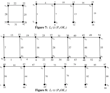
Example 2.10. A one modulo three root square mean labeling of L2 ∪(P4 ʘK1) and L7 ∪(P6 ʘK1) are shown in figure 7 and figure 8 respectively.
Figure 7: L2 ∪ (P4 ʘK1)
Figure 8: L7 ∪ (P6ʘK1)
s1
t1
84 75
72 63
60
58
55 66 69 78 81
79 73
67 61
64 70 76 82
s2 s3 s4 s5
t2 t3 t4 t5
s6 87
88
90
t6 85
u1
u2 u3 u4 u5 u6 u7
v1
v2 v3 v4 v5 v6 v7
1
0 1 6 30 39 48 57
9 15 21 27 36 45 54
4 22 34 43 52
55 46
37 28
16 10
7
13 19 25 31 40 49
28 22 21
33 31
25 22
28
u1 u2
v2
v1 s1
t1
19 13
7 0
1
1 6 12 18
16 10
4
7 13 19
s2 s3 s4
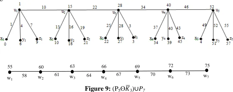
Theorem 2.11. (Pm ʘ$%3) ∪ Pn is a one modulo three root square mean graph.
Proof: Let u1u2 …. um be the path Pm. Let vi, xi, yi, zi be the vertices of ith copy of K1, 3
with central vertex vi. Identifyvi with ui, 1≤ i ≤ m.Let w1w2…wn be the path Pn. The
resultant graph is G = (Pm ʘ$%3) ∪ Pn with V(G) ={ui, xi, yi, zi, wj /1≤ i≤ m, 1≤ j≤ n} and
E(G) = {uixi, uiyi, uizi, ujuj+1, wjwj+1 / 1≤ i ≤ m, 1≤ j≤ n-1}. Then G has 4m+n vertices and
4m+n-2 edges. Define a function ϕ: V(G) → {0, 1, 3,…, 3q-2, 3q} by ϕ(u1) = 1; ϕ(u2) =
15; ϕ(ui) =12i-8, 3≤ i≤ m; ϕ(x1) = 0; ϕ(xi) =12i-14, 2≤ i ≤ m; ϕ(y1)= 6; ϕ(y2) =16; ϕ(yi) =
12i-9, 3≤ i ≤ m; ϕ(zi) = 12i-3, 1≤ i≤ m; ϕ(w1)= 12m-5, ϕ(wi)= 12m+3i-6, 2≤ i ≤ n. Then ϕ
induces a bijection ϕ*: E(G) → {1, 4, …, 3q-2}, where ϕ*(uiui+1)=12i-2, 1≤ i≤ m-1;
ϕ*(uixi)=12i-11, 1≤ i ≤ m; ϕ*(uiyi)=12i-8, 1≤ i ≤ m; ϕ*(uizi) =12i-5, 1≤ i ≤ m; ϕ*(wiwi+1)
=12m+3i-5, 1≤ i ≤ n-1. Therefore, ϕ is a one modulo three root square mean labeling. Hence (Pm ʘ$%3) ∪ Pn is a one modulo three root square mean graph.
Example 2.12. One modulo three root square mean labeling of (P5 ʘ$%3)∪P7 is given in
figure 6.
Figure 9: (P5ʘ$%3)∪P7
3. Conclusion
In this paper, we prove that some disconnected graphs (Lm ʘK1) ∪ Pn, (Lm
ʘK1) ∪(PnʘK1), Pn ∪Pm, Lm ∪ (PnʘK1), (Pm ʘ$%3) ∪ Pn and Lm ∪ Pn, for m 2 and n 3
are one modulo three root square mean labeling.
Acknowledgement. The authors would like to thank reviewer(s) of this article for the time they spent and for their valuable suggestions which improved the presentation of the work.
REFERENCES
1. F. Harary, Graph theory, Narosa Publishing House, New Delhi (1998).
2. J.A.Gallian, A dynamic survey of graph labeling, The Electronics Journal of Combinatorics, 17 (2014).
3. M.Pal, Intersection graphs: An introduction, Annals of Pure and Applied Mathematics, 4 (1) (2013) 41 – 93.
4. A.Saha, M.Pal and T.K.Pal, Selection of programme slots of television channels for giving advertisement: A graph theoretic approach, Information Sciences, 177 (12) (2007) 2480 -2492.
75 73 72
70 69 67 66
64 63 60
55
58 61
5. C.David Raj and C.Jayasekaran, Some results on one modulo three harmonic mean graphs, International Journal of Mathematical Archieve, 5 (2014) 203-208.
6. S.S.Sandhya, S.Somasundaram and S.Anusa, Root square mean labeling of graphs, International Journal of Contemporary Mathematical Sciences, 9 (2014) 667-676. 7. C.Jayasekaran and M. Jaslin Melbha, One modulo three root square mean labeling of
path related graphs, to appear in International Journal of Pure and Applied Mathematics.