The Thirty-Third AAAI Conference on Artificial Intelligence (AAAI-19)
Learning Dynamic Generator Model
by Alternating Back-Propagation through Time
Jianwen Xie,
1∗Ruiqi Gao,
2∗Zilong Zheng,
2Song-Chun Zhu,
2Ying Nian Wu
21Hikvision Research Institute, Santa Clara, USA2University of California, Los Angeles, USA
Abstract
This paper studies the dynamic generator model for spatial-temporal processes such as dynamic textures and action se-quences in video data. In this model, each time frame of the video sequence is generated by a generator model, which is a non-linear transformation of a latent state vector, where the non-linear transformation is parametrized by a top-down neu-ral network. The sequence of latent state vectors follows a non-linear auto-regressive model, where the state vector of the next frame is a non-linear transformation of the state tor of the current frame as well as an independent noise vec-tor that provides randomness in the transition. The non-linear transformation of this transition model can be parametrized by a feedforward neural network. We show that this model can be learned by an alternating back-propagation through time algorithm that iteratively samples the noise vectors and updates the parameters in the transition model and the gen-erator model. We show that our training method can learn realistic models for dynamic textures and action patterns.
1
Introduction
1.1
The model
Most physical phenomena in our visual environments are spatial-temporal processes. In this paper, we study a gener-ative model for spatial-temporal processes such as dynamic textures and action sequences in video data. The model is a non-linear generalization of the linear state space model proposed by (Doretto et al. 2003) for dynamic textures. The model of (Doretto et al. 2003) is a hidden Markov model, which consists of a transition model that governs the transi-tion probability distributransi-tion in the state space, and an emis-sion model that generates the observed signal by a map-ping from the state space to the signal space. In the model of (Doretto et al. 2003), the transition model is an auto-regressive model in thed-dimensional state space, and the emission model is a linear mapping from thed-dimensional state vector to theD-dimensional image. In (Doretto et al. 2003), the emission model is learned by treating all the frames of the input video sequence as independent obser-vations, and the linear mapping is learned by principal com-ponent analysis via singular value decomposition. This
re-∗
Equal contributions
Copyright c2019, Association for the Advancement of Artificial Intelligence (www.aaai.org). All rights reserved.
duces the D-dimensional image to a d-dimensional state vector. The transition model is then learned on the sequence of d-dimensional state vectors by a first order linear auto-regressive model.
Given the high approximation capacity of the modern deep neural networks, it is natural to replace the linear struc-tures in the transition and emission models of (Doretto et al. 2003) by the neural networks. This leads to the follow-ing dynamic generator model that has the followfollow-ing two components. (1) The emission model, which is a generator network that maps thed-dimensional state vector to theD -dimensional image via a top-down deconvolution network. (2) The transition model, where the state vector of the next frame is obtained by a non-linear transformation of the state vector of the current frame as well as an independent Gaus-sian white noise vector that provides randomness in the tran-sition. The non-linear transformation can be parametrized by a feedforward neural network or multi-layer perceptron. In this model, the latent random vectors that generate the ob-served data are the independent Gaussian noise vectors, also called innovation vectors in (Doretto et al. 2003). The state vectors and the images can be deterministically computed from these noise vectors.
1.2
The learning algorithm
Such dynamic models have been studied in the computer vi-sion literature recently, notably (Tulyakov et al. 2017). How-ever, the models are usually trained by the generative adver-sarial networks (GAN) (Goodfellow et al. 2014) with an ex-tra discriminator network that seeks to distinguish between the observed data and the synthesized data generated by the dynamic model. Such a model may also be learned by vari-ational auencoder (VAE) (Kingma and Welling 2014) to-gether with an inference model that infers the sequence of noise vectors from the sequence of observed frames. Such an inference model may require a sophisticated design.
distribution of the noise vectors can be calculated by back-propagation through time. (2) Learning back-back-propagation through time, which updates the parameters of the transition model and the emission model by gradient ascent, where the gradient of the log-likelihood with respect to the model parameters can again be calculated by back-propagation through time.
The alternating back-propagation (ABP) algorithm was originally proposed for the static generator network (Han et al. 2017). In this paper, we show that it can be general-ized to the dynamic generator model. In our experiments, we show that we can learn the dynamic generator models using the ABPTT algorithm for dynamic textures and action sequences.
Two advantages of the ABPTT algorithm for the dynamic generator models are convenience and efficiency. The al-gorithm can be easily implemented without designing an extra network. Because it only involves back-propagations through time with respect to a single model, the computa-tion is very efficient.
1.3
Related work
The proposed learning method is related to the following themes of research.
Dynamic textures. The original dynamic texture model (Doretto et al. 2003) is linear in both the transition model and the emission model. Our work is concerned with a dy-namic model with non-linear transition and emission mod-els. See also (Tesfaldet, Brubaker, and Derpanis 2018) and references therein for some recent work on dynamic tex-tures.
Chaos modeling. The non-linear dynamic generator model has been used to approximate chaos in a recent pa-per (Pathak et al. 2017). In the chaos model, the innovation vectors are given as inputs, and the model is deterministic. In contrast, in the model studied in this paper, the innova-tion vectors are independent Gaussian noise vectors, and the model is stochastic.
GAN and VAE.The dynamic generator model can also be learned by GAN or VAE. See (Tulyakov et al. 2017) (Saito, Matsumoto, and Saito 2017) and (Vondrick, Pirsiavash, and Torralba 2016) for recent video generative models based on GAN. However, GAN does not infer the latent noise vectors. In VAE (Kingma and Welling 2014), one needs to design an inference model for the sequence of noise vectors, which is a non-trivial task due to the complex dependency structure. Our method does not require an extra model such as a dis-criminator in GAN or an inference model in VAE.
Models based on spatial-temporal filters or kernels.The patterns in the video data can also be modeled by spatial-temporal filters by treating the data as 3D (2 spatial dimen-sions and 1 temporal dimension), such as a 3D energy-based model (Xie, Zhu, and Wu 2017) where the energy function is parametrized by a 3D bottom-up ConvNet, or a 3D gen-erator model (Han et al. 2019) where a top-down 3D Con-vNet maps a latent random vector to the observed video data. Such models do not have a dynamic structure defined by a transition model, and they are not convenient for predicting future frames.
1.4
Contribution
The main contribution of this paper lies in the combination of the dynamic generator model and the alternating back-propagation through time algorithm. Both the model and al-gorithm are simple and natural, and their combination can be very useful for modeling and analyzing spatial-temporal processes. The model is one-piece in the sense that (1) the transition model and emission model are integrated into a single latent variable model. (2) The learning of the dy-namic model is end-to-end, which is different from (Han et al. 2017)’s treatment. (3) The learning of our model does not need to recruit a discriminative network (like GAN) or an in-ference network (like VAE), which makes our method sim-ple and efficient in terms of computational cost and model parameter size.
2
Model and learning algorithm
2.1
Dynamic generator model
LetX = (xt, t= 1, ..., T)be the observed video sequence, wherextis a frame at timet. The dynamic generator model consists of the following two components:
st=Fα(st−1, ξt), (1)
xt=Gβ(st) +t, (2) wheret= 1, ..., T. (1) is the transition model, and (2) is the emission model.stis thed-dimensional hidden state vector.
ξt ∼ N(0, I)is the noise vector of a certain dimensional-ity. The Gaussian noise vectors(ξt, t = 1, ..., T)are inde-pendent of each other. The sequence of (st, t = 1, ..., T) follows a non-linear auto-regressive model, where the noise vectorξtencodes the randomness in the transition fromst−1
tostin thed-dimensional state space.Fαis a feedforward neural network or multi-layer perceptron, whereαdenotes the weight and bias parameters of the network. We can adopt a residual form (He et al. 2016) forFαto model the change of the state vector.xtis theD-dimensional image, which is generated by thed-dimensional hidden state vectorst.Gβis a top-down convolutional network (sometimes also called deconvolution network), where β denotes the weight and bias parameters of this top-down network.t∼N(0, σ2ID) is the residual error. We letθ= (α, β)denote all the model parameters.
Letξ= (ξt, t= 1, ..., T).ξconsists of the latent random vectors that need to be inferred fromX. Althoughxtis gen-erated by the state vectorst,S = (st, t= 1, ..., T)are gen-erated byξ. In fact, we can writeX=Hθ(ξ) +, whereHθ composesFαandGβover time, and= (t, t= 1, ..., T) denotes the observation errors.
2.2
Learning and inference algorithm
Let p(ξ) be the prior distribution of ξ. Let pθ(X|ξ) ∼ N(Hθ(ξ), σ2I) be the conditional distribution of X given
ξ, where I is the identity matrix whose dimension matches that ofX. The marginal distribution is pθ(X) =
R
logpθ(ξ, X), where pθ(ξ, X) = p(ξ)pθ(X|ξ), is analyti-cally tractable. The following identity links the gradient of the observed-data log-likelihoodlogpθ(X)to the gradient of the complete-data log-likelihoodlogpθ(ξ, X):
∂
∂θlogpθ(X) = 1 pθ(X)
∂ ∂θpθ(X)
= 1
pθ(X)
Z h
∂
∂θlogpθ(ξ, X) i
pθ(ξ, X)dξ
= Epθ(ξ|X)
h∂
∂θlogpθ(ξ, X) i
, (3)
wherepθ(ξ|X) =pθ(ξ, X)/pθ(X)is the posterior distribu-tion of the latentξgiven the observedX. The above expec-tation can be approximated by Monte Carlo average. Specif-ically, we sample from the posterior distributionpθ(ξ|X) us-ing the Langevin dynamics:
ξ(τ+1)=ξ(τ)+δ
2
2 ∂
∂ξ logpθ(ξ
(τ)|X) +δz
τ, (4)
whereτindexes the time step of the Langevin dynamics (not to be confused with the time step of the dynamics model,
t),zτ ∼ N(0, I)whereI is the identity matrix whose di-mension matches that ofξ, andξ(τ) = (ξ(τ)
t , t = 1, ..., T) denotes all the sampled latent noise vectors at time stepτ.
δ is the step size of the Langevin dynamics. We can cor-rect for the finite step size by adding a Metropolis-Hastings acceptance-rejection step. After samplingξ∼pθ(ξ|X) us-ing the Langevin dynamics, we can updateθby stochastic gradient ascent
∆θ∝ ∂
∂θlogpθ(ξ, X), (5)
where the stochasticity of the gradient ascent comes from the fact that we use Monte Carlo to approximate the expecta-tion in (3). The learning algorithm iterates the following two steps. (1) Inference step: Given the currentθ, sampleξfrom
pθ(ξ|X)according to (4). (2) Learning step: Givenξ, update
θaccording to (5). We can use a warm start scheme for sam-pling in step (1). Specifically, when running the Langevin dynamics, we start from the currentξ, and run a finite num-ber of steps. Then we updateθin step (2) using the sampled
ξ. Such a stochastic gradient ascent algorithm has been ana-lyzed by (Younes 1999).
Since ∂ξ∂ logpθ(ξ|X) = ∂ξ∂ logpθ(ξ, X), both steps (1) and (2) involve derivatives of
logpθ(ξ, X) =−1 2 h
kξk2+ 1
σ2kX−Hθ(ξ)k
2i+ const,
where the constant term does not depend on ξ or θ. Step (1) needs to compute the derivative of logpθ(ξ, X) with respect to ξ. Step (2) needs to compute the derivative of
logpθ(ξ, X) with respect to θ. Both can be computed by back-propagation through time. Therefore the algorithm is an alternating back-propagation through time algorithm. Step (1) can be called inferential back-propagation through time. Step (2) can be called learning back-propagation through time.
To be more specific, the complete-data log-likelihood
logpθ(ξ, X)can be written as (up to an additive constant, assumingσ2= 1)
L(θ, ξ) =−1 2
T
X
t=1
kxt−Gβ(st)k2+kξtk2
. (6)
The derivative with respect toβis
∂L ∂β =
T
X
t=1
(xt−Gβ(st))
∂Gβ(st)
∂β . (7)
The derivative with respect toαis
∂L ∂α =
T
X
t=1
(xt−Gβ(st))
∂Gβ(st)
∂st
∂st
∂α, (8)
where ∂st
∂α can be computed recursively. To inferξ, for any fixed time pointt0,
∂L ∂ξt0
= T
X
t=t0+1
(xt−Gβ(st))
∂Gβ(st)
∂st
∂st
∂ξt0
−ξt0, (9)
where ∂st
∂ξt0
can again be computed recursively.
A minor issue is the initialization of the transition model. We may assume thats0∼N(0, I). In the inference step, we
can samples0together withξusing the Langevin dynamics.
It is worth mentioning the difference between our algo-rithm and the variational inference. While variational infer-ence is convenient for learning a regular generator network, for the dynamic generator model studied in this paper, it is not a simple task to design an inference model that infers the sequence of latent vectorsξ = (ξt, t = 1, ..., T)from the sequence of X = (xt, t = 1, ..., T). In contrast, our learning method does not require such an inference model and can be easily implemented. The inference step in our model can be done via directly sampling from the posterior distributionpθ(ξ|X), which is powered by back-propagation through time. Additionally, our model directly targets maxi-mum likelihood, while model learning via variational infer-ence is to maximize a lower bound.
2.3
Learning from multiple sequences
We can learn the model from multiple sequences of differ-ent appearances but of similar motion patterns. LetX(i)=
(x(ti), t= 1, ..., T)be thei-th training sequence,i= 1, ..., n. We can use an appearance (or content) vectora(i)for each
sequence to account for the variation in appearance. The model is of the following form
s(ti)=Fα(s
(i)
t−1, ξ (i)
t ), (10)
x(ti)=Gβ(s
(i)
t , a
(i)) +(i)
t , (11)
wherea(i)∼N(0, I), anda(i)is fixed over time for each se-quencei. To learn from such training data, we only need to add the Langevin sampling ofa(i). If the motion sequences
of motion patterns, so that the transition model becomes
s(ti)=Fα(s
(i)
t−1, ξ (i)
t , m(i))withm(i)fixed for the sequence
i.
Recently (Tulyakov et al. 2017) studies a similar model where the transition model is modeled by a recurrent neu-ral network (RNN) with another layer of hidden vectors. (Tulyakov et al. 2017) learns the model using GAN. In comparison, we use a simpler Markov transition model and we learn the model by alternating back-propagation through time. Even though the latent state vectors follow a Marko-vian model, the observed sequence is non-MarkoMarko-vian.
Algorithm 1 Learning and inference by alternating back-propagation through time (ABPTT)
Input: (1) training sequences {X(i) = (x(ti), t = 1, ..., T), i= 1, ..., n}
(2) number of Langevin stepsl
(3) number of learning iterationsN.
Output: (1) learned parametersθ= (α, β)
(2) inferred noise vectorsξ(i)= (ξ(i)
t , t= 1, ..., T).
1: Initialize θ = (α, β). Initializeξ(i) anda(i). Initialize k= 0.
2: repeat
3: Inferential back-propagation through time: For
i = 1, ..., n, sampleξ(i) anda(i)by runningl steps of Langevin dynamics according to (4), starting from their current values.
4: Learning back-propagation through time: Update
αandβby gradient ascent according to (8) and (7). 5: Letk←k+ 1
6: untilk=N
Algorithm 1 summarizes the learning and inference algo-rithm for multiple sequences with appearance vectors. If we learn from a single sequence such as dynamic texture, we can remove the appearance vectora(i), or simply fix it to a
zero vector.
3
Related models
In this section, we shall review related models of spatial-temporal processes in order to put our work into the big pic-ture.
3.1
Two related spatial-temporal models
LetX = (xt, t = 1, ..., T)be the observed sequence. We have studied the following energy-based model (Xie, Zhu, and Wu 2017):
p(X;θ) = 1
Z(θ)exp [fθ(X)], (12)
wherefθ(X)is a function of the whole sequenceX, which can be defined by a bottom-up network that consists of mul-tiple layers of temporal filters that capture the spatial-temporal patterns inX at multiple layers.θcollects all the weight and bias parameters of the bottom-up network. The
model can be learned by maximum likelihood, and the learn-ing algorithm follows an “analysis by synthesis” scheme. The algorithm iterates (1) Synthesis: generating synthesized sequences from the current model by Langevin dynamics. (2) Analysis: updating θ based on the difference between the observed sequences and synthesized sequences. The two steps play an adversarial game with fθ serving as a critic. The synthesis step seeks to modify the synthesized examples to increasefθscores of the synthesized examples, while the analysis step seeks to modifyθto increase thefθscores of the observed examples relative to the synthesized examples. We have also studied the following generator model (Han et al. 2019)
s∼N(0, Id), X =gθ(s) +, (13) where the latent state vector sis defined for the whole se-quence, and is assumed to follow a prior distribution which isd-dimensional Gaussian white noise. The whole sequence is then generated by a functiongθ(s)that can be defined by a top-down network that consists of multiple layers of spatial-temporal kernels.θcollects all the weight and bias parame-ters of the top-down network.is the Gaussian noise image sequence. This generator model can be learned by maximum likelihood, and the learning algorithm follows the alternating back-propagation method of (Han et al. 2017).
In (Xie et al. 2018), we show that we can learn the above two models simultaneously using a cooperative learning scheme. We can also cooperatively train the energy-based model (12) and the dynamic generator model (1) and (2) studied in this paper simultaneously, where the dynamic generator model serves as an approximate sampler of the energy-based model.
Unlike the dynamic generator model (1) and (2) studied in this paper, the above two models (12) and (13) are not of a dynamic or causal nature in that they do not directly evolve or unfold over time.
3.2
Action, control, policy, and cost
If we observe the sequence of actionsa= (at, t= 1, ..., T) applied to the system, we can extend the forward dynamic model (1) to
st=Fα(st−1, at, ξt). (14) The model can still be learned by alternating back-propagation through time. With a properly defined cost func-tion, we can optimize the sequencea = (at, t = 1, ..., T) for control. We may also learn a policyπ(at|st−1)directly
from demonstrations by expert controllers. We may call the resulting model that consists of both dynamics and control policy as the controlled dynamic generator model.
We can also learn the cost function from expert demon-strations by inverse reinforcement learning (Ziebart et al. 2008) (Abbeel and Ng 2004), where we can general-ize the above energy-based model (12) to pθ(X,a) =
1
Z(θ)exp[fθ(X,a)], where−fθ(X,a)can be interpreted as
3.3
Velocity field, optical flow, and physics
In our work, the training data are image frames of video se-quences. If we are given the velocity fields over time, we can also learn the dynamic generator model from such data, such as turbulence. Even with raw image sequences, it may still be desirable to learn a model that generates the velocity fields or optical flows over time, which in turn generate the image frames over time. This will lead to a more physically meaningful model of motion, which can be considered the mental physics. In our recent work on deformable genera-tor network (Xing et al. 2018), we model the deformations explicitly. We can combine the deformable generator model and the dynamic generator model. We may also consider re-stricting the transition model to be linear to make the state vector close to real physical variables.
4
Experiments
4.1
Experiment 1: Learn to generate dynamic
textures
We first learn the model for dynamic textures, which are se-quences of images of moving scenes that exhibit stationar-ity in time. We learn a separate model from each example. The video clips for training are collected from DynTex++ dataset of (Ghanem and Ahuja 2010) and the Internet. Each observed video clip is prepared to be of the size 64 pixels × 64 pixels × 60 frames. We implement our model and learning algorithm in Python with Tensorflow (Abadi and et al. 2015). The transition model is a feedforward neu-ral network with three layers. The network takes a 100-dimensional state vectorst−1 and a 100-dimensional noise
vector ξt as input and produces a 100-dimensional vector
rt, so thatst = tanh(st−1+rt). The numbers of nodes in the three layers of the feedforward neural network are {20,20,100}. The emission model is a top-down deconvo-lution neural network or generator model that maps the 100-dimensional state vector (i.e., 1 ×1 ×100) to the image frame of size 64×64×3 by 6 layers of deconvolutions with kernel size of 4 and up-sampling factor of 2 from top to bottom. The numbers of channels at different layers of the generator are{512,512,256,128,64,3}. Batch normaliza-tion (Ioffe and Szegedy 2015) and ReLU layers are added between deconvolution layers, and tanh activation function is used at the bottom layer to make the output signals fall within[−1,1]. We use the Adam (Kingma and Ba 2015) for optimization withβ1 = 0.5and the learning rate is 0.002.
We set the Langevin step size to beδ = 0.03for all latent variables, and the standard deviation of residual errorσ= 1. We runl= 15steps of Langevin dynamics for inference of the latent noise vectors within each learning iteration.
Once the model is learned, we can synthesize dynamic textures from the learned model by firstly randomly initial-izing the initial hidden states0, and then following Equation
(1) and (2) to generate a sequence of images with a sequence of innovation vectors{ξt}sampled from Gaussian distribu-tion. In practice, we use ”burn-in” to throw away some it-erations at the beginning of the dynamic process to ensure the transition model enters the high probability region (i.e.,
the state sequence{st}converges to stationarity), no matter wheres0starts from.
To speed up the training process and relieve the bur-den of computer memory, we can use truncated back-propagation through time in training our model. That is, we divide the whole training sequence into different non-overlapped chunks, and run forward and backward passes through chunks of the sequence instead of the whole se-quence. We carry hidden states{st}forward in time forever, but only back-propagate for the length (the number of image frames) of chunk. In this experiment, the length of chunk is set to be 30 image frames.
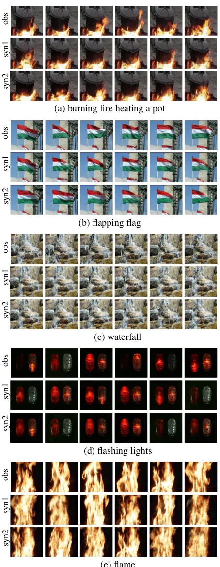
An “infinite length” dynamic texture can be synthesized from a typically “short” input sequence by just drawing “infinite” IID samples from Gaussian distribution. Figure 1 shows five results. For each example, the first row displays 6 frames of the observed 60-frame sequence, while the sec-ond and third rows display 6 frames of two synthesized se-quences of 120 frames in length, which are generated by the learned model.
Similar to (Tesfaldet, Brubaker, and Derpanis 2018), we perform a human perceptual study to evaluate the perceived realism of the synthesized examples. We randomly select 20 different human users. Each user is sequentially presented a pair of synthesized and real dynamic textures in a ran-dom order, and asked to select which one is fake after view-ing them for a specified exposure time. The “foolview-ing” rate, which is the user error rate in discriminating real versus syn-thesized dynamic textures, is calculated to measure the re-alism of the synthesized results. Higher “fooling” rate in-dicates more realistic and convincing synthesized dynamic textures. “Perfect” synthesized results corresponds to a fool-ing rate of 50% (i.e., random guess), meanfool-ing that the users are unable to distinguish between the synthesized and real examples. The number of pairwise comparisons presented to each user is 36 (12 categories×3 examples). The expo-sure time is chosen from discrete durations between 0.3 and 3.6 seconds.
We compare our model with three baseline methods, such as LDS (linear dynamic system) (Doretto et al. 2003), TwoStream (Tesfaldet, Brubaker, and Derpanis 2018) and MoCoGAN (Tulyakov et al. 2017), for dynamic texture syn-thesis in terms of “fooling” rate on 12 dynamic texture videos (e.g., waterfall, burning fire, waving flag, etc).
LDS represents dynamic textures by a linear autoregres-sive model; TwoStream method synthesizes dynamic tex-tures by matching the feature statistics extracted from two pre-trained convolutional networks between synthesized and observed examples; and MoCoGAN is a motion and content decomposed generative adversarial network for video gen-eration.
obs
syn1
syn2
(a) burning fire heating a pot
obs
syn1
syn2
(b) flapping flag
obs
syn1
syn2
(c) waterfall
obs
syn1
syn2
(d) flashing lights
obs
syn1
syn2
(e) flame
Figure 1: Generating dynamic textures. For each category, the first row displays 6 frames of the observed sequence, and the second and third rows show the corresponding frames of two synthesized sequences generated by the learned model.
300 600 1200 2400 3600 Exposure time (ms)
0.0 0.1 0.2 0.3 0.4 0.5
Fool rate / User error
Method Ours Doretto MoCoGAN TwoStream
Figure 2: Limited time pairwise comparison results. Each curve shows the “fooling” rates (realism) over different ex-posure times.
realistic dynamic textures than other baseline methods. The result also shows that the linear model (i.e., LDS) outper-forms the more sophisticated baselines (i.e., TwoStream and MoCoGAN). The reason is because when learning from a single example, the MoCoGAN may not fit the training data very well due to the unstable and complicated adversarial training scheme as well as a large number of parameters to be learned, and the TwoStream method has a limitation that it cannot handle dynamic textures that have structured back-ground (e.g., burning fire heating a pot).
4.2
Experiment 2: Learn to generate action
patterns with appearance consistency
We learn the model from multiple examples with different appearances by using a 100-dimensional appearance vector. We infer the appearance vector and the initial state via a 15-step Langevin dynamics within each iteration of the learn-ing process. We learn the model uslearn-ing the Weizmann ac-tion dataset (Gorelick et al. 2007), which contains 81 videos of 9 people performing 9 actions, including jacking, jump-ing, walkjump-ing, etc, as well as an animal action dataset that includes 20 videos of 10 animals performing running and walking collected from the Internet. Each video is scaled to
64×64pixels×30frames. We adopt the same structure of the model as the one in Section 4.1, except that the emis-sion model takes the concatenation of the appearance vector and the hidden state as input. For each experiment, a single model is trained on the whole dataset without annotations. The dimensions of the hidden statesand the Gaussian noise
ξ are set to be 100 and 50 respectively for the Weizmann action dataset, and 3 and 100 for the animal action dataset.
Figure 3 shows some synthesized results for each experi-ment. To synthesize video, we randomly pick an appearance vector inferred from the observed video and generate new motion pattern for that specified appearance vector by the learned model with a noise sequence of {ξt, t = 1, .., T} and an initial states0sampled from Gaussian white noise.
We show two different synthesized motions for each appear-ance vector. With a fixed appearappear-ance, the learned model can generate diverse motions with consistent appearance.
syn1
syn2
person 1
syn1
syn2
person 2
(a) synthesizing human actions (Weizmann dataset)
syn1
syn2
lion
syn1
syn2
tiger
(b) synthesizing animal actions (animal action dataset)
Figure 3: Generated action patterns. For each inferred ap-pearance vector, two synthesized videos are displayed.
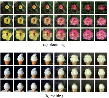
interpolating between appearance vectors of videos at the two ends. We conduct these experiments on some videos selected from categories “blooming” and “melting” in the dataset of (Zhou and Berg 2016). For each example, the videos at the two ends are generated with the appearance vectors inferred from two observed videos. Each video in the middle is obtained by first interpolating the appearance vec-tors of the two end videos, and then generating the videos using the dynamic generator. All the generated videos use the same set of noise sequence{ξt}ands0randomly
sam-pled from Gaussian white noise. We observe smooth transi-tions in contents and motransi-tions of all the generated videos and that the intermediate videos are also physically plausible.
We compare with MoCoGAN and TGAN (Saito, Mat-sumoto, and Saito 2017) by training on 9 selected cate-gories (e.g., PlayingCello, PlayingDaf, PlayingDhol, ingFlute, PlayingGuitar, PlayingPiano, PlayingSitar, Play-ingTabla, and PlayingViolin) of videos in the UCF101 (Soomro, Zamir, and Shah 2012) database and following (Saito, Matsumoto, and Saito 2017) to compute the incep-tion score. Table 1 shows comparison results. Our model
(a) blooming
(b) melting
Figure 4: Video interpolation by interpolating between ap-pearance latent vectors of videos at the two ends. For each example, each column is one synthesized video. We show 3 frames for each video in each column.
outperforms the MoCoGAN and TGAN in terms of incep-tion score.
Table 1: Inception score for models trained on 9 classes of videos in UCF101 database.
Reference ours MoCoGAN TGAN
11.05±0.16 8.21±0.09 4.40±0.04 5.48±0.06
4.3
Experiment 3: Learn from incomplete data
Our model can learn from videos with occluded pixels and frames. We adapt our algorithm to this task with mini-mal modification involving the computation ofPT
t=1kxt−
Gβ(st)k2. In the setting of learning from fully observed videos, it is computed by summing over all the pixels of the video frames, while in the setting of learning from partially visible videos, we compute it by summing over only the vis-ible pixels of the video frames. Then we can continue to use the alternating back-propagation through time (ABPTT) al-gorithm to infer{ξt, t= 1, ..., T}ands0, and then learnβ
andα. With inferred{ξt}ands0, and learnedβ andα, the
video with occluded pixels or frames can be automatically recovered byGβ(st), where the hidden state can be recur-sively computed byst=Fα(st−1, ξt).
(a) ocean
(b) playing
(c) windmill
(d) flag
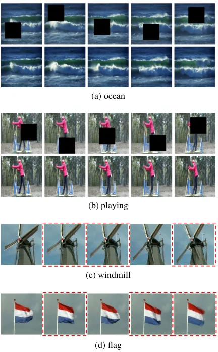
Figure 5: Learning from occluded videos. (a,b) For each ex-periment, the first row displays a segment of the occluded sequence with black masks. The second row shows the cor-responding segment of the recovered sequence. (c,d) The 3 frames with red bounding box are recovered by the learning algorithm, and they are occluded in the training stage. Each video has 70 frames and 50%frames are randomly occluded.
worth mentioning that learning from incomplete data can be difficult for GANs (e.g., MoCoGAN), because of their lack of an adaptive inference process in the training stage. Here “adaptive” means the inference can be performed on input images with different sets of occluded pixels.
We test our recovery algorithm on 6 video sequences collected from DynTex++ dataset. Each input video is of the size 150 pixels ×150 pixels ×70 frames. The emis-sion model is a top-down deconvolutional neural network that maps a 100-dimensional state vector st to the image frame of size150×150×70by 7 layers of deconvolutions with numbers of channels {512,512,256,128,64,64,3}, kernel sizes {4,4,4,4,4,4,7}, and up-sampling factors {2,2,2,2,3,3,1}at different layers from top to bottom. We use the same transition model and the same parameter set-ting as in Section 4.1, except that the standard deviation of residual error isσ= 0.5. We run 7,000 iterations to recover each video. The length of chunk is 70.
We have two types of occlusions: (1) single region mask occlusion, where a 60×60 mask is randomly placed on each150×150image frame of each video. (2) missing im-age frames, where 50%of the image frames are randomly blocked in each video. For each type of occlusion experi-ment, we measure the recovery errors by the average per pixel difference between the recovered video sequences and the original ones (The range of pixel intensities is [0, 255]), and compare with STGCN (Xie, Zhu, and Wu 2017), which is a spatial-temporal deep convolutional energy-based model that can recover missing pixels of videos by synthesis dur-ing the learndur-ing process. We also report results obtained by generic spatial-temporal Markov random field models with potentials that are`1or`2difference between pixels of
near-est neighbors that are defined in both spatial and temporal domains, and the recovery is accomplished by synthesizing missing pixels via Gibbs sampling. Table 2 shows the com-parison results. Some qualitative results for recovery by our models are displayed in Figure 5.
Table 2: Recovery errors in occlusion experiments
(a) single region masks
ours STGCN MRF-`1 MRF-`2
flag 7.8782 8.1636 10.6586 12.5300
fountain 5.6988 6.0323 11.8299 12.1696
ocean 3.3966 3.4842 8.7498 9.8078
playing 4.9251 6.1575 15.6296 15.7085 sea world 5.6596 5.8850 12.0297 12.2868 windmill 6.6827 7.8858 11.7355 13.2036
Avg. 5.7068 6.2681 11.7722 12.6177
(b) 50%missing frames
ours STGCN MRF-`1 MRF-`2
flag 5.0874 5.5992 10.7171 12.6317
fountain 5.5669 8.0531 19.4331 13.2251
ocean 3.3666 4.0428 9.0838 9.8913
playing 5.2563 7.6103 22.2827 17.5692 sea world 4.0682 5.4348 13.5101 12.9305 windmill 6.9267 7.5346 13.3364 12.9911
Avg. 5.0454 6.3791 14.7272 13.2065
4.4
Experiment 4: Learn to remove content
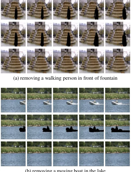
The dynamic generarator model can be used to remove un-desirable content in the video for background inpainting. The basic idea is as follows. We first manually mask the un-desirable moving object in each frame of the video, and then learn the model from the masked video with the recovery al-gorithm that we used in Section 4.3. Since there are neither clues in the masked video nor prior knowledge to infer the occluded object, it turns out to be that the recovery algorithm will inpaint the empty region with the background.
(a) removing a walking person in front of fountain
(b) removing a moving boat in the lake
Figure 6: Learn to remove content for background inpaint-ing. For each experiment, the first row displays 5 image frames of the original video. The second row displays the corresponding image frames with black mask occluding the target to be removed. The third row shows the inpainting re-sults by our method. (a) walking person. (b) moving boat.
size is128×128×104in example (a) and128×128×150in example (b). We adopt the same transition model as the one in Section 4.3, and an emission model that has 7 layers of deconvolutions with kernel size of 4, up-sampling factor of 2, and numbers of channels{512,512,512,256,128,64,3} at different layers from top to bottom. The emission model maps the 100-dimensional state vector to the image frame of size128×128pixels.
The experiment is different from the background inpaint-ing by (Xie, Zhu, and Wu 2017), where the empty regions of the video are inpainted by directly sampling from a prob-ability distribution of pixels in empty region conditioned on visible pixels. As to our model, we inpaint the empty regions of the video by inferring all the latent variables by Langevin dynamics.
4.5
Experiment 5: Learn to animate static image
A conditional version of the dynamic generator model can be used for video prediction given a static image. Specif-ically, we learn a mapping from a static image frame to the subsequent frames. We incorporate an extra encoderEγ, whereγdenotes the weight and bias parameters of the
en-coder, to map the first image framex(0i)into its appearance
or content vectora(i)and state vectors(i)
0 . The dynamic
gen-erator takes the state vectors(0i)as the initial state and uses the appearance vectora(i)to generate the subsequent video
frames {x(ti), t = 1, ..., T} for the i-th video. The condi-tional model is of the following form
[s(0i), a(i)] =Eγ(x
(i)
0 ), (15)
s(ti)=Fα(s
(i)
t−1, ξ (i)
t ), (16)
x(ti)=Gβ(s
(i)
t , a
(i)) +(i)
t . (17)
We learn both the encoder and the dynamic generator (i.e., transition model and emission model) together by alternat-ing back-propagation through time. The appearance vector and the initial state are no longer hidden variables that need to be inferred in training. Once the model is learned, given a testing static image, the learned encoderEγ extracts from it the appearance vector and the initial state vector, which generate a sequence of images by the dynamic generator.
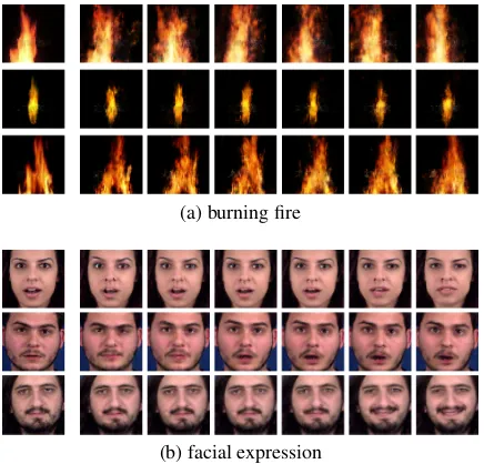
We test our model on burning fire dataset (Xie, Zhu, and Wu 2017), and MUG Facial Expression dataset (N. Aifanti and Delopoulos 2010). The encoder has 3 convolutional lay-ers with numblay-ers of channels {64,128,256}, filter sizes {5,3,3}and sub-sampling factors{2,2,1}at different lay-ers, and one fully connected layer with the output size equal to the dimension of the appearance vector (100) plus the di-mension of the hidden state (80). The didi-mension ofξis 20. The other configurations are similar to what we used in Sec-tion 4.2. We qualitatively display some results in Figure 7, where each row is one example of image-to-video predic-tion. For each example, the left image is the static image frame for testing, and the rest are 6 frames of the predicted video sequence. The results show that the predicted frames by our method have fairly plausible motions.
5
Conclusion
This paper studies a dynamic generator model for spatial-temporal processes. The model is a non-linear generalization of the linear state space model where the non-linear trans-formations in the transition and emission models are param-eterized by neural networks. The model can be conveniently and efficiently learned by an alternating back-propagation through time (ABPTT) algorithm that alternatively samples from the posterior distribution of the latent noise vectors and then updates the model parameters. The model can be gen-eralized by including random vectors to account for various sources of variations, and the learning algorithm can still ap-ply to the generalized models.
Project page
The code and more results can be found at http://www.stat.ucla. edu/∼jxie/DynamicGenerator/DynamicGenerator.html
Acknowledgement
(a) burning fire
(b) facial expression
Figure 7: Image-to-video prediction. For each example, the first image is the static image frame, and the rest are 6 frames of the predicted sequence.
The work is supported by DARPA XAI project N66001-17-2-4029; ARO project W911NF1810296; ONR MURI project N00014-16-1-2007; and a Hikvision gift to UCLA.
We gratefully acknowledge the support of NVIDIA Corporation with the donation of the Titan Xp GPU used for this research.
References
Abadi, M., and et al. 2015. TensorFlow: Large-scale machine learning on heterogeneous systems. Software available from ten-sorflow.org.
Abbeel, P., and Ng, A. Y. 2004. Apprenticeship learning via in-verse reinforcement learning. InProceedings of the Twenty-first International Conference on Machine Learning (ICML), 1–8. Braham, M., and Van Droogenbroeck, M. 2016. Deep background subtraction with scene-specific convolutional neural networks. In
International Conference on Systems, Signals and Image Process-ing (IWSSIP), 1–4.
Doretto, G.; Chiuso, A.; Wu, Y. N.; and Soatto, S. 2003. Dynamic textures.International Journal of Computer Vision51(2):91–109. Ghanem, B., and Ahuja, N. 2010. Maximum margin distance learn-ing for dynamic texture recognition. InEuropean Conference on Computer Vision (ECCV), 223–236.
Goodfellow, I.; Pouget-Abadie, J.; Mirza, M.; Xu, B.; Warde-Farley, D.; Ozair, S.; Courville, A.; and Bengio, Y. 2014. Gen-erative adversarial nets. InAdvances in Neural Information Pro-cessing Systems (NIPS), 2672–2680.
Gorelick, L.; Blank, M.; Shechtman, E.; Irani, M.; and Basri, R. 2007. Actions as space-time shapes.IEEE transactions on pattern analysis and machine intelligence29(12):2247–2253.
Han, T.; Lu, Y.; Zhu, S.-C.; and Wu, Y. N. 2017. Alternating back-propagation for generator network. In31st AAAI Conference on Artificial Intelligence.
Han, T.; Lu, Y.; Xing, X.; and Wu, Y. N. 2019. Learning genera-tor networks for dynamic patterns. InIEEE Winter Conference on Applications of Computer Vision (WACV).
He, K.; Zhang, X.; Ren, S.; and Sun, J. 2016. Deep residual learn-ing for image recognition. InProceedings of the IEEE conference on computer vision and pattern recognition, 770–778.
Ioffe, S., and Szegedy, C. 2015. Batch normalization: Accelerating deep network training by reducing internal covariate shift. arXiv preprint arXiv:1502.03167.
Kingma, D. P., and Ba, J. 2015. Adam: A method for stochastic optimization. InInternational Conference on Learning Represen-tations (ICLR).
Kingma, D. P., and Welling, M. 2014. Auto-encoding variational bayes. InInternational Conference on Learning Representations (ICLR).
N. Aifanti, C. P., and Delopoulos, A. 2010. The MUG facial ex-pression database. InProceedings of 11th Int. Workshop on Image Analysis for Multimedia Interactive Services (WIAMIS), 12–14. Pathak, J.; Lu, Z.; Hunt, B. R.; Girvan, M.; and Ott, E. 2017. Using machine learning to replicate chaotic attractors and calculate lya-punov exponents from data. Chaos: An Interdisciplinary Journal of Nonlinear Science27(12):121102.
Saito, M.; Matsumoto, E.; and Saito, S. 2017. Temporal generative adversarial nets with singular value clipping. InIEEE International Conference on Computer Vision (ICCV).
Soomro, K.; Zamir, A. R.; and Shah, M. 2012. Ucf101: A dataset of 101 human actions classes from videos in the wild.arXiv preprint arXiv:1212.0402.
Tesfaldet, M.; Brubaker, M. A.; and Derpanis, K. G. 2018. Two-stream convolutional networks for dynamic texture synthesis. In
IEEE Conference on Computer Vision and Pattern Recognition (CVPR).
Tulyakov, S.; Liu, M.-Y.; Yang, X.; and Kautz, J. 2017. Moco-gan: Decomposing motion and content for video generation.arXiv preprint arXiv:1707.04993.
Vondrick, C.; Pirsiavash, H.; and Torralba, A. 2016. Generating videos with scene dynamics. InAdvances In Neural Information Processing Systems (NIPS), 613–621.
Xie, J.; Lu, Y.; Gao, R.; Zhu, S.-C.; and Wu, Y. N. 2018. Coopera-tive training of descriptor and generator networks. IEEE Transac-tions on Pattern Analysis and Machine Intelligence(preprints). Xie, J.; Zhu, S.-C.; and Wu, Y. N. 2017. Synthesizing dynamic patterns by spatial-temporal generative convnet. InProceedings of the IEEE Conference on Computer Vision and Pattern Recognition (CVPR), 7093–7101.
Xing, X.; Gao, R.; Han, T.; Zhu, S.-C.; and Wu, Y. N. 2018. De-formable generator network: Unsupervised disentanglement of ap-pearance and geometry.arXiv preprint arXiv:1806.06298. Younes, L. 1999. On the convergence of markovian stochastic algorithms with rapidly decreasing ergodicity rates. Stochastics: An International Journal of Probability and Stochastic Processes
65(3-4):177–228.
Zhou, Y., and Berg, T. L. 2016. Learning temporal transformations from time-lapse videos. InEuropean Conference on Computer Vi-sion (ECCV), 262–277.