R E S E A R C H
Open Access
A new extragradient-like method for solving
variational inequality problems
Na Huang
1, Changfeng Ma
1*and Zhenggang Liu
2*Correspondence: [email protected] 1School of Mathematics and Computer Science, Fujian Normal University, Fuzhou, 350007, China Full list of author information is available at the end of the article
Abstract
In this paper, we present a new extragradient-like method for the classical variational inequality problem based on our constructed novel descent direction. Furthermore, we show the global convergence and R-linear convergence rate of the new method under certain conditions. Numerical results also confirm the good theoretical properties of our approach.
MSC: 90C33; 65K10
Keywords: variational inequality problem; extragradient-like method; global convergence; R-linear convergence; numerical experiment
1 Introduction
In this paper, we consider the classical variational inequality problem, which is to find a vectorx*∈Ksuch that
Fx*,x–x*≥, ∀x∈K, (.)
whereFis a continuous mapping fromRnintoRn,Kis a nonempty closed convex subset ofRn, and·,·is the usual Euclidean inner product inRn. We denote problem (.) by VI(F,K) and its solution set byK*. VI(F,K) was first introduced by Hartman and Stam-pacchia (see []) in , primarily with the goal of computing stationary points for non-linear programs. It provides a broad unifying setting for the study of optimization and equilibrium problems and servers as the main computational framework for the practical solution of a host of continuum problems in the mathematical sciences. It has a wide range of important applications in economics, engineering, operations researchetc.; we will not dwell further on this. The problem we are interested in is how to find the vectorx*∈K*.
Recently, there have been many methods proposed in the literature to tackle this prob-lem (see []), among which we think the projection method is one of the most excel-lent ones. The projection method for solving problem (.) came originally from the Goldstein (see []) and Levitin-Polyak (see []) gradient projection method for the box-constrained minimization and was studied by many researchers such as Auslender (see []), Bakusinskii-Polyak (see []), Bruck (see []), Noor-Wang-Xiu (see []) and Xiu-Wang-Zhang (see []). Its original iterative scheme is finding anxk∈Ksuch that
xk+=PK
xk–αFxk, k= , , , . . . , (.)
wherePK[·] is the orthogonal projection fromRnontoK, andα> is a fixed number. Korpelevich (see []) combined two neighboring iterations in (.) and then got a new projection method:
⎧ ⎨ ⎩
¯ xk=P
K[xk–αF(xk)],
xk+=P
K[xk–αF(¯xk)].
(.)
That is the extragradient method which has R-linear convergence rate. The vector –F(¯xk) in (.) is the descent direction off(x) =x–x*(x∈K,x*∈K*) at a pointxk under certain conditions, which is the key to the convergence of the algorithm. There are several studies on the descent direction. To our knowledge, just five descent directions are found so far (see [, –]). In this paper, we construct a novel descent direction and present a new extragradient-like method based on the direction. Furthermore, we prove that the new method has the same R-linear convergence rate as the extragradient method. Some numerical experiments are given to prove our analysis.
The rest of this article is organized as follows. In Section , some preliminaries are stated and an extragradient-like method is proposed. In Section , the global convergence and the local convergence rate of the algorithm are proved. The results of some preliminary experiments on a few test examples are reported in Section , and the conclusions are given in Section .
2 Preliminaries and algorithm
We first provide some necessary conclusions from convex analysis and related papers.
Definition . K is a nonempty closed convex subset ofRn,x∈K is the projection of y∈RnontoKif
x=arg minz–y|z∈K.
Then callxasPK[y].
Definition . C⊂Rnis a nonempty subset,F(x) is a mapping fromCintoRn.F(x) is pseudomonotone onCif for allx,y∈C,x=y, the following implication relation is estab-lished:
(x–y)TF(y)≥ ⇒ (x–y)TF(x)≥.
Lemma . The variational inequality(.)has a solution x*∈K*if and only if x*satisfies the relation
x*=PK
x*–αFx*,
whereα> is a constant and PK[·]is an orthogonal projection from Rnonto K.
inequalities. To prove the convergence and convergence rate of our algorithm later, the other two lemmas are presented here.
Lemma .(Property .. in []) Let PK[·]be the projection from Rnonto K,then for y,z∈Rn,
PK[y] –PK[z]
≤y–z,PK[y] –PK[z]
.
Specially,it follows from the Cauchy-Schwarz inequality that
PK[y] –PK[z]≤ y–z.
Lemma .(Property .. in []) Let PK[·]be the projection from Rnonto K,take x∈K and d∈Rnarbitrarily,then
() x–PK[x–αd]
α is monotonic nonincreasing on the variableα> .
() x–PK[x–αd]is monotonic nondecreasing on the variableα> .
Lemma . For anyα> and x∈Rn,
min{,α}e(x, )≤e(x,α)≤max{,α}e(x, ),
where e(x,α) =x–PK[x–αF(x)].
Proof Ifα≤, from Lemma ., we know thate(x,α)is monotonic nondecreasing and
e(x,α)
α is monotonic nonincreasing on the variableα> . Then we have e(x,α)≤e(x, )=max{,α}e(x, )
and
e(x,α)
min{,α}=
e(x,α)
α ≥
e(x, )
=e(x, ).
Combining the above two inequalities, we can easily get the result.
From the same argument, we can get the result if α> . Summing up the two cases
completes the proof.
Now, we begin to establish the following iterative method for solving problem (.).
Algorithm .(A new extragradient-like method)
Step (Initialization) Choose the initial valuesx∈Rn,l∈(, ),μ∈(, ) andθ∈(, ], take the stopping criterion> . Setk:= .
Step (The predictor step) Compute the predictor
¯ xk=PK
xk–αkF
xk, (.)
whereαk=lmk andmkis the smallest nonnegative integermsuch that
Fxk–Fx¯k≤μx k–x¯k
αk
Step (The corrector step) Computing the corrector
xk+=PK
xk–βkdk
, (.)
where
dk=αk
( –θ)Fxk+θFx¯k, (.)
βk=θ( –μ)x k–x¯k
dk . (.)
Step Ifxk+–xk ≤, then stop; otherwise, setk:=k+ go to Step .
Remark . To our knowledge, the search directiondkin Algorithm . is new; moreover, –dkis a descent direction off(x) =
x–x*(x∈K,x*∈K*) at a pointxkunder certain conditions. We will prove it in the next section.
Remark . IfF(xk) = , thenF(xk),x–x*= ,∀x∈K, namelyxk∈K*, so the algo-rithm will be stopped. Therefore,F(xk)= when the algorithm is running, by (.) and Lemma ., we have
( –θ)Fxk+θFx¯k=Fxk–θFxk–Fx¯k ≥Fxk–θFxk–Fx¯k
≥Fxk–θ μ αk
xk–x¯k
≥Fxk–θ μFxk
= ( –θ μ)Fxk> .
Thus by (.) we getdk> in the algorithm, that is, Step of Algorithm . is well posed.
3 Convergence analysis
In this section, we discuss the convergence and convergence rate of Algorithm .. Firstly, we prove an important lemma.
Lemma . Assume that F(x)is pseudomonotone on K and K*is nonempty.If xk∈K is not a solution to problem(.),then for any x*∈K*,
dk,xk–x*≥θ( –μ)xk–x¯k. (.)
Proof Takex*∈K*arbitrarily. Asx*∈K*, we have
Fx*,x–x*≥, ∀x∈K.
Specially, forxk∈Kandx¯k∈K, we can get
and
Fx*,x¯k–x*≥.
From the pseudomonotonicity ofF(x), we have
Fxk,xk–x*≥ (.)
and
Fx¯k,x¯k–x*≥. (.)
From Lemma . we get
xk–x¯k≤xk–xk–αkF
xk,xk–x¯k
=αkF
xk,xk–x¯k
=αk
Fxk,xk–x¯k,
namely
Fxk,xk–x¯k≥x k–x¯k
αk
. (.)
By the Cauchy-Schwarz inequality and (.), we get
Fxk–Fx¯k,xk–x¯k≤Fxk–Fx¯k·xk–x¯k
≤μx k–x¯k
αk
. (.)
Combining (.), (.) and (.) yields
Fx¯k,xk–x*≥Fx¯k,xk–x¯k
=Fxk,xk–x¯k–Fxk–Fx¯k,xk–x¯k
≥xk–x¯k αk
–μx k–x¯k
αk
= ( –μ)x k–x¯k
αk
. (.)
Thus, from (.), (.), (.) andθ∈(, ], we obtain
dk,xk–x*=αk
( –θ)Fxk+θFx¯k,xk–x*
= ( –θ)αk
Fxk,xk–x*+θ αk
Fx¯k,xk–x*
≥θ( –μ)xk–x¯k,
By using Lemma . and the proof technique usual in projection-type methods, we easily conclude the global convergence of Algorithm ..
Theorem . Assume that F(x) is continuous and pseudomonotone on K and K* is nonempty.If{xk}and{¯xk}are two infinite sequences produced by Algorithm.,then
lim
k→∞
xk–x¯k= , (.)
and{xk}converges to a solution of problem(.).
Proof For anyx*∈K*, it follows from (.), (.), Lemma . and Lemma . that for allk,
xk+–x*≤xk–βkdk–x*
=xk–x*– βk
dk,xk–x*+βkdk
≤xk–x*– θ( –μ)βkxk–x¯k
+βkdk
=xk–x*–θ( –μ)x k–x¯k
dk . (.)
Thus, the sequence{xk}generated by Algorithm . is bounded, and
θ( –μ)
∞
k=
xk–x¯k dk ≤
∞
k=
xk–x*–xk+–x*<∞.
So xk–¯xk
dk → ask→ ∞. Notice thatF(x) is continuous onK,PK[·] is continuous on Rnand{xk} ⊆Kis bounded, the sequence{¯xk}is bounded, thereby the sequence{dk}is bounded. Then we have
xk–x¯k=x k–x¯k dk ·d
k
→, k→ ∞,
and then we get the (.). Supposelimki→∞xki=x∞, we will prove thatx∞∈K*.
Ifαki≥αmin> , from Lemma . we can get
ex∞, = lim
ki→∞
exki, ≤ lim
ki→∞
xki–x¯ki min{,αmin}
= .
Ifαki→, for all sufficiently largeki, it follows from (.) and Lemma .() that
μexki, ≤μe(x
ki,αki
l )
αki
l
<Fxki–F
xki
αki
l
,
wherexki(αki
l ) =PK[x ki–αki
l F(x ki)], so
ex∞, = lim
ki→∞
exki, ≤ lim
ki→∞
F(xki) –F(xki(αki
l ))
In both cases, we havee(x∞, )= . From Lemma . we havex∞∈K*. Combining it with (.), we obtain
xk+–x∞≤xk–x∞–θ( –μ)x k–x¯k dk ≤x
k–x∞ .
Then∀k= , , . . . , choosekij∈ {ki}satisfyingkij≤k, we can get
xk+–x∞≤xk–x∞≤ · · · ≤xkij–x∞,
thus,{xk}converges to a solution of problem (.).
From Theorem ., we can easily get the following result.
Corollary . Assume that F(x) is continuous and pseudomonotone on K and K* is nonempty.If{xk}is an infinite sequence produced by Algorithm.,then
lim
k→∞x
k+–xk= .
Proof From (.), (.) and Lemma ., we have
xk+–xk=PK
xk–βkdk
–xk≤βkdk
=θ( –μ)x k–x¯k
dk .
From the proving process of Theorem ., we have
lim
k→∞
xk–x¯k dk = ,
which implies that
lim
k→∞
xk–x¯k dk = .
That is,xk+–xk → ask→+∞.
The above corollary shows that Algorithm . is terminable. The following theorem im-plies that Algorithm . has R-linear convergence rate.
Theorem . Assume that variational inequality problemVI(F,K)meets the following conditions:
(a) F(x)is pseudomonotone onKandK*is nonempty; (b) F(x)is Lipschitz continuous onKwith Lip-constantL> ;
(c) the local error bound holds,that is,there exist constantsτ> andδ> such that
If{xk}is an infinite sequence produced by Algorithm.,then it converges to a solution of (.)R-linearly.
Proof From the condition (b) and (.), we can easily get
μx
k–xk(αk
l )
αk
l
<Fxk–F
xk
αk l
≤Lxk–xk
αk l
.
After appropriate simplification, we get
αk≥ lμ
L :=α, ∀k= , , , . . . .
Then by Lemma . and Theorem ., we have
exk, ≤ x k–x¯k
min{,αk}≤
xk–x¯k
min{,α} →. (.)
So, there exists sufficiently largeksuch that
exk, ≤δ, ∀k≥k.
Thus, from the condition (c), we get
distxk,K*≤τexk, , ∀k≥k. (.)
From the proving process of Theorem ., we know that{dk}is bounded, so there exists a constantM> such thatdk ≤M. Choosingx*∈K*closest toxk, from (.), (.) and (.), we obtain for allk≥k,
distxk+,K*≤xk+–x*
≤xk–x*–θ( –μ)x k–x¯k dk
≤distxk,K*–θ( –μ)(min{,α})
τ
[dist(xk,K*)] dk
≤
–θ( –μ)(min{,α})
τ
[dist(xk,K*)] M
distxk,K*.
Thus,{dist(xk,K*)}converge to zero at a Q-linear rate, then the desired result follows.
4 Numerical examples
iterations (Iter.), CPU time (CPU) and residual error (Err.). All computations were done using the PC with Intel(R) Core(TM)i CPU M @ . GHz. All the programming is implemented in MATLAB Rb.
Throughout the computational experiments, unless otherwise stated, the parameters in Algorithm . were set asl= . andμ= .. As the descent directiondkchanges with the parameterθ, we use differentθin different experiments and then find something interesting.
Example . This test problem is from Ahn (see []). LetF(x) =Mx+q, where
M= ⎛ ⎜ ⎜ ⎜ ⎜ ⎜ ⎜ ⎜ ⎜ ⎜ ⎜ ⎜ ⎝ – – . .. . .. ... ... . .. – ⎞ ⎟ ⎟ ⎟ ⎟ ⎟ ⎟ ⎟ ⎟ ⎟ ⎟ ⎟ ⎠
, q=
⎛ ⎜ ⎜ ⎜ ⎜ ⎜ ⎜ ⎜ ⎜ ⎜ ⎜ ⎜ ⎝ – – .. . .. . .. . – ⎞ ⎟ ⎟ ⎟ ⎟ ⎟ ⎟ ⎟ ⎟ ⎟ ⎟ ⎟ ⎠ .
We test this problem by usingx= (, , . . . , )Tas a starting point and set the parameter θ= . for different dimensionsn. The test results are listed in Table .
Example . This problem was tested by Kanzow (see []) with five variables defined by
Fi(x) = (xi–i+ )exp
j=
(xj–j+ )
, ≤i≤.
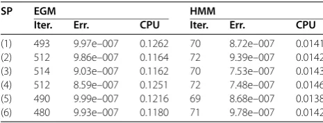
This example has one degenerate solutionx*= (, , , , )T. The numerical results are given in Table using different start points (SP). The parameterθ= . in this example as well.
Table 1 Numerical results for Example 4.1
DIM EGM HMM
Iter. Err. CPU Iter. Err. CPU
256 131 9.96e–007 1.3014 20 6.30e–007 0.2013 512 136 9.08e–007 6.2570 20 6.41e–007 0.9330 1024 139 9.86e–007 24.6350 20 6.71e–007 3.5909 2048 143 9.47e–007 99.7605 20 6.81e–007 14.2013 4096 146 9.80e–007 406.0588 20 7.20e–007 56.4115
Table 2 Numerical results for Example 4.2
SP EGM HMM
Iter. Err. CPU Iter. Err. CPU
(1, 0, 1, 3, 5)T 63 7.60e–007 0.0282 27 9.33e–007 0.0058
(1, 2, 3, 1, 2)T 66 9.32e–007 0.0230 17 9.17e–007 0.0043
(1, 2, 3, 4, 5)T >1000 5.74e+001 0.4057 45 8.49e–007 0.0068
(2, 2, 2, 2, 2)T 70 8.43e–007 0.0224 18 4.56e–007 0.0037
Table 3 Numerical results for Example 4.3
SP EGM HMM
Iter. Err. CPU Iter. Err. CPU
(1) 493 9.97e–007 0.1262 70 8.72e–007 0.0141 (2) 512 9.86e–007 0.1164 72 9.39e–007 0.0142 (3) 514 9.03e–007 0.1162 70 7.53e–007 0.0143 (4) 512 8.59e–007 0.1251 72 7.48e–007 0.0146 (5) 490 9.99e–007 0.1216 69 8.68e–007 0.0138 (6) 480 9.93e–007 0.1180 71 9.78e–007 0.0142
Table 4 Numerical results for Example 4.4
SP EGM HMM
Iter. Err. CPU Iter. Err. CPU
(0, 0, 0, 0)T 193 9.64e–007 0.0230 180 9.85e–007 0.0197
(1, 1, 1, 1)T 206 9.59e–007 0.0309 190 9.54e–007 0.0177
(2, 2, 2, 2)T 92* 9.45e–007 0.0109 37* 7.52e–007 0.0055
(3, 1, 2, 6)T 95* 7.70e–007 0.0134 47* 8.22e–007 0.0065
(6, 1, 6, 6)T 99* 9.14e–007 0.0121 47* 8.30e–007 0.0080
(10, 10, 10, 10)T 214 9.50e–007 0.0284 181 9.89e–007 0.0188
Example . The Nash problem. This is a Nash equilibrium model with ten variables. The test functionF(x) = (F(x), . . . ,F(x))Tis defined by
Fi(x) =ci+ (Lixi) βi –
k=xk
γ
+ xi γk=xk
k=xk
γ
, ≤i≤,
where γ = ., c= (., ., ., ., ., ., ., ., ., .)T, L
i = (≤i≤) and β= (., ., ., ., ., ., ., ., ., .)T. The test results for Example . are sum-marized in Table using the following standard starting points: ()e; () e; () e; () e; () (., ., ., ., ., ., ., ., ., .)T; () (, , , , , , , , , )T. This time we set θ= ..
Example . The Kojshin problem. This example was used by Pang and Gabriel (see []), and Kanzow (see []) with four variables. Let
F(x) =
⎛ ⎜ ⎜ ⎜ ⎝
x
+ xx+ x+x+ x– x
+x+x+ x+ x– x+xx+ x+ x+ x–
x+ x+ x+ x–
⎞ ⎟ ⎟ ⎟ ⎠.
This problem has one degenerate solution (
√
, , ,
)T and one nondegenerate solu-tion (, , , )T. The numerical results are listed in Table using different initial points. The asterisk (*) denotes that the limit point generated by the algorithms is the degenerate solution; otherwise, it is the nondegenerate solution. We also setθ= . in this example.
Table 5 Numerical results for Example 4.5 withK= [0, 5]4
SP EGM HMM
Iter. Err. CPU Iter. Err. CPU
(1, 1, 1, 1)T 155 9.92e–007 0.0490 25 7.38e–007 0.0032 (–2, –2, –2, –2)T 137 9.47e–007 0.0445 15 4.72e–007 0.0029 (10, 10, 10, 10)T 174 9.58e–007 0.0469 32 2.26e–007 0.0044
(–2, –2, 6, 6)T 172 9.47e–007 0.0567 27 9.74e–007 0.0043
(8, 3, –1, –3)T 159 9.81e–007 0.0519 15 3.77e–007 0.0032
(10, –10, –10, 10)T 183 9.32e–007 0.0580 26 4.57e–007 0.0037
Table 6 Numerical results for Example 4.5 withK= [–1, 1]4
SP EGM HMM
Iter. Err. CPU Iter. Err. CPU
(0.5, 0.5, 0.5, 0.5)T 70 8.73e–007 0.0217 18 4.67e–007 0.0028
(–2, –2, –2, –2)T 59 8.94e–007 0.0138 16 8.04e–007 0.0024
(10, 10, 10, 10)T 76 9.72e–007 0.0283 19 4.84e–007 0.0026
(–2, –2, 6, 6)T 63 7.73e–007 0.0141 13 6.97e–007 0.0032
(8, 3, –1, –3)T 76 9.97e–007 0.0254 18 7.42e–007 0.0031
(10, –10, –10, 10)T 59 8.94e–007 0.0150 18 4.96e–007 0.0030
follows:
F(x) =
⎛ ⎜ ⎜ ⎜ ⎝
x– x–x+x
+ x+x+ x–
x+ x
⎞ ⎟ ⎟ ⎟ ⎠.
We consider the following two cases:
() K= [, ]. The solutionx*= (, , , )T,F(x*) = (, , , )Tis degenerate but not R-regular.
() K= [–, ]. The solutionx*= (, –, , )T,F(x*) = (–, , –, )Tis also degenerate but not R-regular.
In the example, the parameterθin Algorithm . is chosen asθ= .. The test results are listed in Table and Table using different starting points forK= [, ]andK= [–, ], respectively.
Example . This is a box-constrained affine variational inequality VI(F,K) with four variables, and the constraint setK= [ai,bi]n,i= , . . . ,nis a box region. The function is given as follows:
F(x) =Mx+q,
where
M=
⎛ ⎜ ⎜ ⎜ ⎝
– – –
⎞ ⎟ ⎟ ⎟
⎠, q=
⎛ ⎜ ⎜ ⎜ ⎝
– – –
Table 7 Numerical results for Example 4.6 withK= [–1, 1]4
SP EGM HMM
Iter. Err. CPU Iter. Err. CPU
(0.5, 0.5, 0.5, 0.5)T 53 8.45e–007 0.0213 30 5.76e–007 0.0059 (–2, –2, –2, –2)T 66 8.30e–007 0.0247 40 4.25e–007 0.0070 (10, 10, 10, 10)T 54 8.73e–007 0.0200 39 2.93e–007 0.0080
(–6, –6, 6, 6)T 62 8.00e–007 0.0249 41 6.95e–007 0.0084
(8, 3, –3, –8)T 57 8.31e–007 0.0223 35 9.39e–007 0.0060
(10, –10, –10, 10)T 60 8.22e–007 0.0211 38 4.04e–007 0.0064
Table 8 Numerical results for Example 4.6 withK= [–5, 5]4
SP EGM HMM
Iter. Err. CPU Iter. Err. CPU
(2, 2, 2, 2)T 119 9.30e–007 0.0316 77 3.62e–007 0.0104 (–2, –2, –2, –2)T 137 8.52e–007 0.0434 77 6.80e–007 0.0109 (10, 10, 10, 10)T 141 9.78e–007 0.0418 78 9.73e–007 0.0107
(–8, –8, –8, –8)T 143 8.37e–007 0.0411 81 9.33e–007 0.0122
(9, 4, –4, –9)T 129 9.87e–007 0.0393 77 8.28e–007 0.0106
(10, –10, –10, 10)T 127 8.09e–007 0.0387 79 5.58e–007 0.0112
We consider the following two cases:
() K= [–, ]. The solutionx*= (, /, /, /)T,F(x*) = (–/, , , )T; () K= [–, ]. The solutionx*= (/, /, /, /)T,F(x*) = (, , , )T.
In the example, the parameterθ in Algorithm . is chosen asθ= .. The test results are listed in Table and Table using different starting points forK= [–, ]andK= [–, ], respectively.
From the above experiments, we find that the newly developed method (Algorithm .) enjoys obvious advantages in the number of iterations and CPU time. In Example ., the iterations of our algorithm always keep with the increasing of dimension, but the extragradient method is growing. What is more, in this example, the CPU time for the extragradient method is seven times than our algorithm. In Example ., although our algorithm’s error is sometimes larger than that of the extragradient method (when the start point is (, , , , )), our algorithm is more steady obviously (when we choose (, , , , )T and (, , , , )Tas start points, the extragradient method does not work). Moreover, the CPU time for our algorithm is just about one sixth of that for the extragradient method. The last two examples are box-constrained variational inequality problems. In these two examples, our algorithm is also obviously advantageous. In addition, the parameterθ is very small, which implies the importance ofF(xk) in the descent directiondk. In some examples we set parameterθsmall enough, however, Algorithm . even works less well than the extragradient method. In a word, our algorithm is promising.
5 Conclusion
some extent. The progress yet needs to be made in the numerical methods of the varia-tional inequality problem.
Competing interests
The authors declare that they have no competing interests.
Authors’ contributions
All authors contributed equally and significantly in writing this article. All authors read and approved the final manuscript.
Author details
1School of Mathematics and Computer Science, Fujian Normal University, Fuzhou, 350007, China.2Faculty of Foreign Languages and Cultures, Kunming University of Science and Technology, Kunming, 650500, China.
Acknowledgements
The project was supported by the National Natural Science Foundation of China (Grant No. 11071041) and Fujian Natural Science Foundation (Grant No. 2009J01002).
Received: 20 August 2012 Accepted: 16 November 2012 Published: 10 December 2012 References
1. Hartman, P, Stampacchia, G: On some nonlinear elliptic differential functional equations. Acta Math.115, 153-188 (1966)
2. Xiu, N, Zhang, J: Some recent advances in projection-type methods for variational inequalities. J. Comput. Appl. Math.
152, 559-585 (2003)
3. Goldstein, AA: Convex programming in Hilbert space. Bull. Am. Math. Soc.70, 709-710 (1964)
4. Levitin, ES, Polyak, BT: Constrained minimization problems. U.S.S.R. Comput. Math. Math. Phys.6, 1-50 (1966) 5. Auslender, A: Optimization Moethodes Numoeriques. Masson, Paris (1976)
6. Bakusinskii, AB, Polyak, BT: On the solution of variational inequalities. Sov. Math. Dokl.15, 1705-1710 (1974) 7. Bruck, RE: An iterative solution of a variational inequality for certain monotone operators in Hilbert space. Bull. Am.
Math. Soc.81, 890-892 (1975)
8. Aslam Noor, M, Wang, Y, Xiu, N: Some new projection methods for variational inequalities. Appl. Math. Comput.137, 423-435 (2003)
9. Xiu, N, Wang, Y, Zhang, X: Modified fixed-point equations and related iterative methods for variational inequalities. Comput. Math. Appl.47, 913-920 (2004)
10. Korpelevich, GM: The extragradient method for finding saddle points and other problems. Matecon12, 747-756 (1976)
11. He, B, Stoer, J: Solution of projection problems over polytopes. Numer. Math.61, 73-90 (1992) 12. He, B: A new method for a class of linear variational inequalities. Math. Program.66, 137-144 (1994)
13. He, B: A class of projection and contraction methods for monotone variational inequalities. Appl. Math. Optim.35(1), 69-76 (1997)
14. Solodov, MV, Tseng, P: Modified projection-type methods for monotone variational inequalities. SIAM J. Control Optim.34(5), 1814-1830 (1996)
15. Sun, D: A class of iterative methods for solving nonlinear projection equations. J. Optim. Theory Appl.91(1), 123-140 (1996)
16. Bello Cruz, JY, Iusem, AN: A strongly convergent direct method for monotone variational inequalities in Hilbert spaces. Numer. Funct. Anal. Optim.30, 23-36 (2009)
17. Bello Cruz, JY, Iusem, AN: Convergence of direct methods for paramonotone variational inequalities. Comput. Optim. Appl.46, 247-263 (2010)
18. Censor, Y, Gibali, A, Reich, S: The subgradient extragradient method for solving variational inequalities in Hilbert space. J. Optim. Theory Appl.148, 318-335 (2011)
19. Iusem, AN: An iterative algorithm for the variational inequality problem. J. Comput. Appl. Math.13, 103-114 (1994) 20. Iusem, AN, Svaiter, BF: A variant of Korpelevich’s method for variational inequalities with a new search strategy.
Optimization42, 309-321 (1997). Addendum Optimization43, 85 (1998)
21. Khobotov, EN: Modifications of the extragradient method for solving variational inequalities and certain optimization problems. U.S.S.R. Comput. Math. Math. Phys.27, 120-127 (1987)
22. Konnov, IV: Combined Relaxation Methods for Variational Inequalities. Springer, Berlin, (2001)
23. Konnov, IV: A class of combined iterative methods for solving variational inequalities. J. Optim. Theory Appl.94, 677-693 (1997)
24. Konnov, IV: A combined relaxation method for variational in- equalities with nonlinear constraints. Math. Program.
80, 239-252 (1998)
25. Korpelevich, GM: The extragradient method for finding saddle points and other problems. Èkon. Mat. Metody12, 747-756 (1976)
26. Marcotte, P: Application of Khobotov’s algorithm to variational inequalities and network equilibrium problems. Inf. Syst. Oper. Res.29, 258-270 (1991)
27. Solodov, MV, Svaiter, BF: A new projection method for monotone variational inequality problems. SIAM J. Control Optim.37, 765-776 (1999)
28. Solodov, MV, Tseng, P: Modified projection-type methods for monotone variational inequalities. SIAM J. Control Optim.34, 1814-1830 (1996)
30. Ahn, BH: Iterative methods for linear complementarity problem with upperbounds and lowerbounds. Math. Program.26, 265-315 (1983)
31. Kanzow, C: Some equation-based methods for the nonlinear complementarity problem. Optim. Methods Softw.3, 327-340 (1994)
32. Pang, J-S, Gabriel, SA: NE/SQP: a robust algorithm for the nonlinear complementarity problem. Math. Program.60, 295-337 (1993)
doi:10.1186/1687-1812-2012-223

![Table 5 Numerical results for Example 4.5 with K = [0,5]4](https://thumb-us.123doks.com/thumbv2/123dok_us/9682212.1951197/11.595.160.433.225.313/table-numerical-results-example-k.webp)
![Table 7 Numerical results for Example 4.6 with K = [–1,1]4](https://thumb-us.123doks.com/thumbv2/123dok_us/9682212.1951197/12.595.159.434.222.309/table-numerical-results-example-k.webp)
