Adaptive Sparse Confidence-Weighted Learning for Online Feature Selection

(1)

The Thirty-Third AAAI Conference on Artificial Intelligence (AAAI-19)

Adaptive Sparse Confidence-Weighted Learning for Online Feature Selection

Yanbin Liu,

1,2

_{Yan Yan,}

2

_{Ling Chen,}

2

_{Yahong Han,}

3

_{Yi Yang}

2

1_{SUSTech-UTS Joint Centre of CIS, Southern University of Science and Technology} 2_{Centre for Artificial Intelligence, University of Technology Sydney}

3_{College of Intelligence and Computing, Tianjin University}

{csyanbin, yanyan.tju}@gmail.com, [email protected], [email protected], [email protected]

Abstract

In this paper, we propose a new online feature selection algo-rithm for streaming data. We aim to focus on the following two problems which remain unaddressed in literature. First, most existing online feature selection algorithms merely uti-lize the first-order information of the data streams, regardless of the fact that second-order information explores the corre-lations between features and significantly improves the per-formance. Second, most online feature selection algorithms are based on the balanced data presumption, which is not true in many real-world applications. For example, in fraud de-tection, the number of positive examples are much less than negative examples because most cases are not fraud. The bal-anced assumption will make the selected features biased to-wards the majority class and fail to detect the fraud cases. We propose an Adaptive Sparse Confidence-Weighted (ASCW) algorithm to solve the aforementioned two problems. We first introduce an `0-norm constraint into the second-order

confidence-weighted (CW) learning for feature selection. Then the original loss is substituted with a cost-sensitive loss function to address the imbalanced data issue. Furthermore, our algorithm maintains multiple sparse CW learner with the corresponding cost vector to dynamically select an optimal cost. We theoretically enhance the theory of sparse CW learn-ing and analyze the performance behavior in F-measure. Em-pirical studies show the superior performance over the state-of-the-art online learning methods in the online-batch setting.

1 Introduction

Online learning typically receives and processes a single instance at a time. It has become extremely popular and been employed in many applications such as video-ad allo-cation (Sumita et al. 2017). In order to deal with high dimen-sional data streams, online feature selection (OFS) has been proposed to select a fixed number of features for prediction by an online learning fashion.

Existing online feature selection algorithms usually apply the first-order updating rule (Wang et al. 2014; Han et al. 2016). For example, OFS (Wang et al. 2014) modified the first-order Perceptron (Rosenblatt 1958) algorithm by apply-ing truncation. However, feature interactions are ignored by these algorithms. Prior studies in online learning have at-tested the effectiveness of second-order algorithms, such as

confidence-weighted (CW) learning (Crammer, Dredze, and Pereira 2009), with a covariance structure exploring the fea-ture correlations. Due to the high computation cost of co-variance matrix, very few methods (Tan et al. 2016) have been advanced for second-order online feature selection.

While class imbalance is prevalent in real-world applica-tions, it remains to be under-studied in the context of online feature selection. Current online learning methods usually combine first-order updating rules with cost-sensitive learn-ing to deal with class imbalance (Wang, Zhao, and Hoi 2014; Zhao and Hoi 2013; Yan et al. 2017). In this sense, how to decide appropriate cost values is the key challenge in these methods. While most algorithms adopt fixed or ad-hoc schemes to compute costs from the given data, OMCSL (Yan et al. 2017) trains a number of classifiers with various costs and achieves improved performance.

To the best of our knowledge, no previous work has un-covered the problem of online feature selection with the presence of class imbalance. Motivated by this, we propose an Adaptive Sparse CW algorithm (ASCW) for imbalanced online-batch feature selection. Specifically, our method si-multaneously maintains multiple sparse CW learners. For each learner, we assign a unique cost vector to its objective function. As the online training proceeds, we incrementally update the target measure for each learner in an online man-ner. For each online-batch, we choose the best performer for prediction. The main contributions of our paper are summa-rized as follows:

• We propose an adaptive sparse CW method for feature selection on imbalanced online-batch data. Unlike pre-vious approaches that use a fixed or ad-hoc cost vector, our method dynamically chooses the best cost from a set of candidates by incrementally updating the target perfor-mance for each learner.

• We enhance the theory of the existing sparse CW feature selection algorithm and analyze the performance behavior for F-measure.

• Empirical studies demonstrate the efficacy of the pro-posed algorithm. Further results show that our algorithm is capable to automatically choose a cost that is suffi-ciently close to the best one.

(2)

formulation and the cost-sensitive sparse CW algorithm for imbalanced feature selection. Next, we show how the adap-tive strategy chooses a cost from candidates and provide the-oretical analysis. We further discuss our experimental results and finally, conclude the paper.

2 Related Work

Online learning has been extensively studied in machine learning community (Crammer et al. 2006; Crammer, Dredze, and Pereira 2009; Wang, Zhao, and Hoi 2012; Crammer, Kulesza, and Dredze 2009; Ma et al. 2010; Dong et al. 2019). First-order algorithms (Crammer et al. 2006; Zinkevich 2003) usually ignore the direction and scale of parameter updates. Confidence-weighted (CW) learning (Crammer, Dredze, and Pereira 2009) addresses this issue by assuming a Gaussian distribution over weights with mean µ ∈ _Rd _{and covariance}_Σ _∈

Rd×d with theoretical

guar-antees in terms of mistake bounds. However, the aggres-sive update rules based on separable data assumption may cause over-fitting for noisy data.Adaptive Regularization of Weights(AROW) (Crammer, Kulesza, and Dredze 2009) re-laxes such separable assumption by employing a soft-margin squared hinge loss plus a confidence penalty. As another so-lution,Soft Confidence-weighted(SCW) (Wang, Zhao, and Hoi 2012) assigns adaptive margins for different instances.

Cost-sensitive approaches have been proposed to deal with imbalanced online learning problem, such as CSOGD (Wang, Zhao, and Hoi 2014), CSOAL (Zhao and Hoi 2013), and MBPA (Han et al. 2016). They either utilize PA (Crammer et al. 2006) or OGD (Zinkevich 2003) updat-ing rules, which only consider the first-order information and ignore covariance structure. ACOG (Zhao et al. 2018) adopts the idea of adaptive regularization to incorporate the second-order information, which is similar to our method. However, they use ad-hoc cost values computed from the training instances while we dynamically choose the optimal cost from a set of candidates.

Many online feature selection methods have been pro-posed recently (Wu et al. 2013; Zhou et al. 2017; Yu et al. 2014; Wang et al. 2014; Han et al. 2016; Wu et al. 2017; Tan et al. 2016), most of which are first-order methods. For example, OFS (Wang et al. 2014) adopts the first-order Per-ceptron (Rosenblatt 1958) updating rule and MBPA (Han et al. 2016) utilizes the first-order PA (Crammer et al. 2006) updating rule. Based on CW learning, (Wu et al. 2017) tries to incorporate the diagonal elements of the covariance ma-trix for online feature selection. However, the feature cor-relations is not fully explored by only using diagonal infor-mation. Compared with the above methods, we not only ex-plore feature correlations by incorporating second-order co-variance structure but also select features that can better fit the imbalanced measures due to the adaptive cost-selection strategy.

3 Imbalanced Online-Batch CW Learning

3.1 Notations

We first present some notations. Let superscriptT _represent transpose, 0 be a vector/matrix with all zeros, k · kp

de-note thelp-norm of a vector, diag(·)be the diagonal matrix,

ABstand for the element-wise product ofAandB, and

I(b) be an indicator function, whereI(b) = 1 ifb is true

and 0 otherwise. Let[n] ={1, . . . , n}.{Xh,yh}denote ex-amples received at theh-th iteration, whereXh ∈ Rd×Nh

and yh ∈ {−1,1}Nh. µh andΣh respectively represent model weights and covariance at theh-th iteration. We de-notefh(Xh) :Rd×Nh _→

RNh_{as the prediction function at}

theh-th iteration andfh=fh(Xh)as the predictions.

3.2 Cost-Sensitive Learning for Imbalanced Data

For traditional confidence-weighted learning (Crammer, Dredze, and Pereira 2009; Wang, Zhao, and Hoi 2012) and high-dimensional online feature selection such as (Tan et al. 2016), the cumulative mistake is optimized by the hinge loss as: `(µ; (xi, yi)) = max(0,1 −yiµTxi). However, for imbalanced feature selection, this loss function ignores cost asymmetry between the majority classes and the mi-nority ones. Thus, we propose the cost-sensitive loss func-tion to deal with the imbalanced problem:`c(µ; (xi, yi)) =

c+I(yi = 1)`(µ; (xi, yi)) +c−I(yi = −1)`(µ; (xi, yi)). Let Di = c+I(yi = 1) + c−I(yi = −1). Then,

`c(µ; (xi, yi)) = Di`(µ; (xi, yi)). Moreover, we also propose `2

c(µ; (xi, yi)) = Di`(µ; (xi, yi))2 as the cost-sensitive squared hinge loss.

Thus, how to choose c+andc− is the key issue for

im-balanced learning. We will describe the choice strategy in section 5, together with a theoretical analysis in detail.

3.3 Online-Batch CW Learning

Inspired by AROW (Crammer, Kulesza, and Dredze 2009) and cost-sensitive learning (Wang, Zhao, and Hoi 2014), we propose an algorithm to estimateµ,Σ at theh-th iteration for online-batch data.

Fixµand updateΣ. We learnΣfor the following prob-lem:

min

Σ DKL(N(µ,Σ)kN(µh−1,Σh−1)) +

C 2

Nh X

i=1

xT_i Σxi,

(1) where DKL:=1₂log(

detΣh−1 detΣ ) +

1 2Tr(Σ

−1

h−1Σ) + 1

2(µh−1−

µ)T_Σ−1

h−1(µh−1−µ)−

d

2. Using KKT condition, we have

Σ−1=Σ−_h₋1₁+CXhXTh. (2)

FixΣand updateµ. Once we getΣ, we can learnµby the following problem:

min µ

1

2(µ−µh−1) T

Σ−_h1(µ−µh−1) +

C q

Nh X

i=1

Di`(µ; (xi, yi))q,

(3) whereq= 1or2.

SinceΣis positive semidefinite (PSD), it can be rewritten asΣ=γ2. We introducew:=γ−1µ,wh−1 :=γ−1µh−1

and_bxi:=γxi, then problem (3) can be reformulated:

min

w

1

2kw−wh−1k 2 2+

C q

Nh X

i=1

(3)

In order to solve problem (4), we assume an online setting, i.e., each example comes sequentially fromi = 1toNh. This setting is similar to PA (Crammer et al. 2006). Thus we can come up with the solution as follows:

w=wh−1+τiyixi, (5)

τi= min(`(w; (xbi, yi))/kbxik 2

2, CDi), forq= 1 ; (6)

τi=`(w; (xbi, yi))/(kbxik 2

2+ 1/(2CDi)), forq= 2. (7)

4 Sparse CW for Feature Selection

4.1 Feature Selection by Sparsity Index

η

The proposed online-batch CW learning algorithm main-tains the full covariance matrix Σ. It is thus not appro-priate for very dimensional data. In practice, high-dimensional data often exhibits the property of having many zero values and only a small number of features are rele-vant (Ma et al. 2009). Usually, only the relerele-vant features and their interactions are significant for specific applica-tions. Based on these observations, we propose the sparse feature selection algorithm in this section.

In order to find the most relevant features, we introduce an index vectorη={0,1}d_{and apply it to the feature vector}_x as(ηx). Hereηj = 1if featurejis selected andηj = 0 otherwise. In this situation, hinge loss is expressed as:

`(µ,η; (xi, yi)) = max(0,1−yiµT(ηxi)). (8)

Thus`c(µ,η; (xi, yi)) =Di`(µ,η; (xi, yi)).

Considering our aim for feature selection, we impose an

`0-norm constraint onηto induce the sparsity property, i.e.,

kηk0 ≤r(whererd). In convenience, letΛ:={η|η∈

{0,1}d_,_k_η_k

0 ≤ r}be the set of all candidate η. So there

are|Λ|=Pr

i=0(

d

i)feasibleηin total, which is exponential. In the following, we will incorporateηinto the online-batch CW learning and solve it gradually.

At first, as in Section 3.3, we assumeµandηare given, and solve forΣ. Accordingly, we incorporateη into equa-tion (1):

min

Σ DKL(N(µ,Σ)kN(µh−1,Σh−1))

+C

2

Nh X

i=1

(ηxi)TΣ(ηxi). (9)

LetXr_h =diag(η)Xh. Applying the KKT condition onΣ, the closed form solution is:

Σ(η)−1=Σ−_h₋1₁+C(Xr_h)(Xr_h)T. (10)

Once we haveΣ(η), we incorporateηinto formulation (3) and obtain the following problem:

min η∈Λminµ

1

2(µ−µh−1)

T_Σ

h(η)−1(µ−µh−1)

+C

q

Nh X

i=1

Di`(µ,η; (xi, yi))q, (11)

whereq= 1or2.

Problem (11) is a mixed integer problem includingηand µ, which is hard to solve. Here, we employ the convex re-laxation proposed in (Tan, Wang, and Tsang 2010) and ap-ply the KKT condition to transform it into the dual form as a standard convex problem (detailed development can be found in Appendix A.1):

max

θ∈R,α∈Aθ , s.t.θ≤f(α, η), ∀η∈Λ. (12)

Here, f(α,η) is defined as: f(α,η) =

−1 2g(α,η)

T_Σ

h(η)g(α,η)−(q−1)α˜

T_α_˜ 2C +

PNh

i=1αi− µT

h−1g(α,η) where g(α,η) :=

PNh

i=1αiyi(η xi), α ∈ RNh _{is the dual variable with regard to equation (8),}

∀i∈[Nh]andA:={α∈RNh_|₀_≤_α

i≤U}is the domain ofα(here,U =CDiforq= 1andU =∞forq= 2). At last,α˜ = [α1/D

1/2

1 , . . . , αNh/D 1/2

Nh].

4.2 Optimization

Problem (12) has exponential number of constraints as

Pr

i=0(

d

i), making it difficult to directly solve. Fortunately, not all constraints in (12) are active at optimality. Alterna-tively, we can efficiently solve this problem by cutting plane algorithm (Kortanek and No 1993), which iteratively gen-erate a pool of sparse feature subsets to constitute the con-straints in (12).

Instead of considering allT =Pr

i=1(

d

i)constraints, we iteratively seek an active constraint until some stopping con-ditions are encountered. Given the previously estimatedα, the most-violated constraint can be found by solving the fol-lowing problem:

ηt= arg min

η∈Λf(α,η)

= arg max

η∈Λg(α,η) T_Σ

h(η)g(α,η) + 2µTh−1g(α,η).

(13)

Lets=PNh

i=1αiyixi, theng(α,η) =ηs.Problem (13) can be reformulated:

ηt= arg max

η∈Λ(s T_Σ

h(η) + 2µTh−1)(ηs). (14)

Letm= (sT_Σ

h(η) + 2µTh−1)s, then this problem can be

solved by finding therfeatures with the largest score (e.g.

mj), and setting the correspondingηj to 1 and the rest to 0. In other words,mj measures the importance of thej-th feature and acts as the feature score.

After we obtained an active constraintηt, it can be added to the active setΛt=Λt−1∪ {ηt}, then we can solve the following subproblem w.r.t constraints defined byΛt:

max

θ∈R,α∈Aθ, s.t.θ≤f(α, η), ∀η∈Λt. (15)

Problem (14) and (15) are solved alternatively and stop when: (1)|θt−θt−1|/|θt| ≤ , whereis small tolerance value; (2) afterm = dp/reiterations in order to choosep

(4)

4.3 Proximal Dual Coordinate Ascent for

Subproblem (15)

Subproblem (15) regarding dual variableαis hard and ex-pensive to directly optimize. So in the following, we give a proximal-dual coordinate ascent based method to efficiently solve it. LetK =|Λt|be the number of active constraints. For each constraintηk ∈Λt, we take out the corresponding data, previous model parameter, model parameter and co-variance matrix w.r.tηk as:xk

i ∈Rr,µ h−1

k ∈R

r_,_µk _∈

Rr

andΣk ∈Rr×r. Furthermore, letγk be the square root of

Σk,wk := γ_k−1µk,w_kh−1 = γ_k−1µh_k−1,xb

k

i = γkTxki. If we denotew = [wk]Kk=1,wh−1 = [wkh−1]

K

k=1 andbxi = [x_bk

i]Kk=1. The loss function`(w,η; (bxi, yi)) = max(0,1−

PK

k=1yiwkTbx

k

i) = max(0,1−yiwTbxi).

The formulation of subproblem (15) is formally similar to the dual format of some problems. By using KKT condition, we can obtain the primal form of subproblem (15) (detailed development can be found in Appendix A.2):

min

w

1 2(

K

X

k=1

kwk−whk−1k)

2₊C q

Nh X

i=1

Di`(w,η; (bxi, yi))

q_.

(16) Problem (16) is non-smooth due to the `2

2,1-norm

regu-larizer. To make this problem tractable, we make some modifications and apply a proximal-dual coordinate ascent method (Shalev-Shwartz and Zhang 2014) to find a nearly accurate solution of (16) effectively. At first, we introduce a small regularization term σ₂kw−wh−1k2(i.e.,σ1) and

address the following optimization problem:

min

w

σ

2kw−wh−1k 2

+1

2(

K

X

k=1

kwk−whk−1k)

2

+C

q

Nh X

i=1

Di`(w,η; (bxi, yi))

q

. (17)

Remark1. Ifw∗is an ₂-accurate minimizer of (17) and the

σwe are choosing is sufficiently small, thenw∗is also an -accurate solution of (16) (Shalev-Shwartz and Zhang 2014). Therefore, the optimal values of problems (16) and (17) are very close.

LetΩ(w) := σ₂kw−wh−1k2+1₂(P

K

k=1kwk−whk−1k)

2_,

and Li(wTbxi) := 1

qDi`(w,η; (xbi, yi))

q_{. Note here} _Ω _is

strongly convex andLiisγ-Lipschitz for someγ >0. Let

Ω∗(z) = maxwwTz−Ω(w)be the conjugate ofΩ(w), and

L∗_i be the conjugate ofLi. Then we can come up with the conjugate dual of problem (17) (detailed development can be found in Appendix A.3):

max

α≥0H(α), (18)

whereH(α) =−Ω∗(CPNh

i=1αibxi)−C

PNh

i=1L∗i(−αi). Following (Shalev-Shwartz and Zhang 2014), we define

z(α) = CPNh

i=1αixbi, then w(α) = ∇

∗_Ω(_z₍_α₎₎_{. Here,}

∇∗_Ω(_z₍_α₎₎_{denotes the gradient of the conjugate of}_Ω_.

Ac-cording to the property of conjugate, it is also the solution

Algorithm 1Imbalanced sparse CW in online-batch manner

Require: ParametersC >0, H, r

Initializeα=_N1

h1,µ0=0,Σ0=I.

forh= 1 :Hdo

Get a batch of data{Xh,yh},whereXh∈Rd×Nh

ComputeΣhby (10) andγby eigen-decomposition. InitializeΛ0=∅andt= 1

whilestopping conditions not meetdo

Findηtby solving (14). LetΛt= Λt−1∪ηt. Computewh_k−1,wh−1according toΛt. Initializez=0,w=wh−1.

fori= 1 :Nhdo ComputeDi,bx

k i.

Compute loss`= max(0,1−PK

k=1yiwTkxb

k i).

if` >0then

Computeαi = min(`/(Ckxbik 2

2), Di)forq =

1orαi=`/(Ckbxik 2

2+ 0.5/Di)forq= 2. Computez=z+Cαixbi.

Computew=w+∇∗_Ω(_z₎_.

end if end for

Updatewh=w, t=t+ 1.

end while

Updateµh=γwh.

end for

ofΩ∗(z) = maxwwTz−Ω(w).1Similarly, we assume an online setting as for problem (4). Finally, we give the full algorithm for solving the imbalanced feature selection prob-lem in Algorithm 1.

4.4 Discussions

We emphasize that the proposed algorithm enhances the the-ory of existing sparse CW (Tan et al. 2016; Wu et al. 2017) methods. First, with the introduction of cost-sensitive loss function in section 3.2, we can select features that better fit the imbalanced measures. Moreover, instead of fixing the cost, we adaptively choose the best cost from candidates and theoretically validate the optimality of our selection method in section 5. Second, in Equation (3) and (11), we employ µh−1as the initialization when updatingµ, while (Tan et al.

2016) uses0. Thusµh−1acts as the warm-start initialization

and further influences on Equation (13) and (14) for solving ηt. (Tan et al. 2016) assumesΣh(η)to be an identity matrix when solving forηt. In fact, it is unclear if this assumption holds in practice. In contrast, we relax such assumption in Eq (13) and (14). Particularly, computing ηt reduces to a simple sorting problem in Eq (14). In intuition, our method takes more advantages of the information from the previous online-batch throughµh−1andΣh(η).

1

(5)

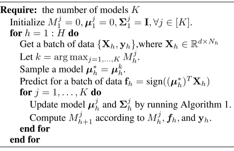
Algorithm 2Multiple Cost-Sensitive Learning.

Require: the number of modelsK

InitializeM₁j= 0,µj₁= 0,Σj₁=I,∀j∈[K]. forh= 1 :Hdo

Get a batch of data{Xh,yh},whereXh∈Rd×Nh

Letk= arg maxj=1,...,KM_hj. Sample a modelµ∗_h=µk_h.

Predict for a batch of datafh=sign((µ∗h)TXh)

forj= 1, . . . , Kdo

Update modelµj_handΣj_hby running Algorithm 1. ComputeM_hj₊₁according toM_hj,fh,andyh.

end for end for

5 Multiple Cost-Sensitive Learning

In section 3 and section 4, we propose the cost-sensitive sparse CW algorithm. However, how to decide the value of c+ andc− remains an issue. Some previous works use

ad-hoc approaches to set up the values (Wang, Zhao, and Hoi 2014; Sahoo, Hoi, and Zhao 2016; Zhao and Hoi 2013). However, there is no guarantee that these approaches can achieve optimal performance for various imbalanced mea-sures such as F-measure, AUPRC, and AUROC.

To solve this problem, we propose a strategy which main-tains multiple cost-sensitive vectors. The motivation is that if multiple cost vectorsc = (c+, c−)is tracked and

main-tained simultaneously, there must exist one setting that can best fit the data. For convenience, we assumec++c− = 1

to eliminate one parameter and thusc+ ∈ (0,1). In order

to maintain the multiplec+, we divide(0,1)intoKevenly

distributed valuesθ1, . . . , θK, i.e.,θj =j/(K+ 1)and set

cj₊ = 1−θj/2, then the cost-sensitive loss is denoted as:

`j_c(µj; (xi, yi)) = (1−θj/2)I(yi= 1)`(µj; (xi, yi))

+ (θj/2)I(yi =−1)`(µj; (xi, yi)). (19)

With this strategy, we can maintain and track K

learners with the corresponding costs simultaneously:

(θ1,µ1), . . . ,(θK,µK). At the h-th online-batch, we up-date the current target measure of thej-th learner, denoted by M_hj. Different from (Yan et al. 2017), we apply the greedy criterion to select the best performer according to

{M_h1, ..., M_hK}fromKcandidates for prediction at theh-th online-batch. With this criterion, we do not need to introduce extra hyper-parameter, and we can analyze the performance guarantee in a different way.

We update the target measures (e.g., F-measure, AUROC, and AUPRC) only using the current measure M_hj, current predictionsfh, and labelsyh, which is efficient without stor-ing allfhandyh. Due to the space limitation, we put the detailed updating formulations in Appendix A.5. We sum-marize the multiple cost-sensitive algorithm in Algorithm 2.

5.1 Theoretical Analysis in F-measure

we define the following notations for binary classification:

a(θ) = [1−θ

2, θ

2]and∆ =

θj−θj+1

2 =

1 2K, P1:the marginal probability of the positive instances,

E(h) = [fn,fp] :false negative and false positive,

F∗= max

e F(e) : the maximum F-measure, F(µ) : the F-measure achieved byµ.

Proposition 1. Assume that {µ1

h, ...,µKh} minimizes the cost-sensitive loss to a certain degree, then the F-measure achieved by Algorithm 2 has the following lower bound as long ashincreases:

max

j=1,...,KF(µ j h)≥F

∗₋_∆₋ 0

P1 ,

wherek= arg maxj=1,...,KF(µ j

h)andha(θk),E(µkh)i ≤

minµha(θk),E(µ)i+0. The full proof is in Appendix A.6.

6 Experiments

In this section, we evaluate the proposed ASCW algorithm on three imbalanced measures, i.e., F-measure, AUROC, and AUPRC and compare with various online learning and feature selection methods.

6.1 Experimental Testbed

We conduct experiments on three widely-used high-dimensional benchmarks and sample with different ratios to construct nine imbalance configurations, as shown in Ta-ble 1. In order to construct imbalanced configurations from the original datasets, we adopt two strategies. Firstly, for bi-nary datasets (real-sim and rcv1), we fix the negative class and sample from the positive class to satisfy specific ratios (1:5, 1:10 and 1:20). Secondly, for the multi-class dataset (news20), we set class1 as positive class and select class2-6, class2-11 and class2-20 as negative class respectively.

Table 1: Datasets Statistics

Datasets d Ntrain

# nonzeros

per example #Pos:#Neg real-sim 20,958 32,309 52 1:5, 1:10, 1:20

rcv1 47,236 20,242 74 1:5, 1:10, 1:20 news20 62,061 15,935 80 1:5, 1:10, 1:19

6.2 Comparison Algorithms

We compare the following algorithms:

• OFS (Wang et al. 2014): The state-of-the-art first-order online feature selection via sparse projection.

• MBPA (Han et al. 2016): Margin-based passive aggres-sive method for online feature selection.

(6)

0 1 2 3

Number of samples ₁₀4 0

0.2 0.4 0.6

Online F-measure

F-measure

0 1 2 3

0.5 1

Online AUROC

AUROC

0 1 2 3

0.2 0.4 0.6

Online AUPRC

AUPRC

OFS MBPA CSOAL SBCW1 SBCW2 ASCW1 ASCW2

(a) real-sim

0 5000 10000 15000 Number of samples 0

0.2 0.4 0.6

Online F-measure

F-measure

0.5 1

Online AUROC

AUROC

0.2 0.4 0.6

Online AUPRC

AUPRC

(b) rcv1

0 5000 10000 Number of samples 0.1

0.2 0.3 0.4

Online F-measure

F-measure

0 5000 10000 Number of samples 0

0.2 0.4 0.6 0.8

Online AUROC

AUROC

0 5000 10000 Number of samples 0

0.1 0.2 0.3 0.4

Online AUPRC

AUPRC

(c) news20

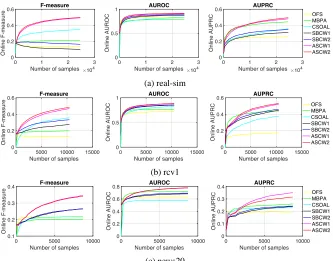
Figure 1: Online performance with imbalance ration 1:10 (other ratios in Appendix A.7) for different performance measures

• SBCW1 and SBCW2 (Tan et al. 2016): Two variations of the sparse online-batch feature selection method.

• FGM (Tan, Tsang, and Wang 2014): The full-batch high-dimensional feature selection method which generates a pool of violated sparse feature subsets and combines them via efficient Multiple Kernel Learning (MKL) algorithm.

• L1SVM (Yuan et al. 2010):`1-norm SVM by Liblinear.

• ASCW1 and ASCW2: The proposed algorithm with hinge (q= 1) and squared hinge (q= 2) loss.

SBCW and ASCW consider second-order structure while others only optimize first-order information.

6.3 Experimental Results

As shown in Table 1, the number of nonzeros per exam-ple varies from 52 to 80 in different datasets, so in the ex-periments we set the selected feature dimension to 50 for all algorithms except that for CSOAL we set query ratio to be 1%.2 _{Following (Hoi, Wang, and Zhao 2014), we}

re-peat all online learning experiments 20 times with random permutation of training data. For full batch methods (FGM, L1SVM), we follow the default settings.

Batch Size.In Algorithm 1, µis updated in a pure on-line manner andΣis updated in an online-batch manner. To explain the necessity of the online-batch update and explore proper batch size, we perform experiments on news20 with various batch sizes, as shown in Table 2. The best perfor-mance is achieved with batch size=1 (the strict online case).

2

Actually, 1% of all examples contain more information than 50 features of entire features for all datasets.

Table 2: Test performance on news20 with various batch sizes

Ratio Batch news20

F AUROC AUPRC Time (s)

1:5

256 0.5614 0.8474 0.6011 0.71 64 0.5640 0.8536 0.6163 2.40 1 0.9125 0.9922 0.9769 913.86

1:10

256 0.4239 0.8114 0.4306 1.39 64 0.4275 0.8096 0.4309 4.53 1 0.8549 0.9872 0.9479 3034.95

1:19

256 0.3349 0.8223 0.3126 2.86 64 0.3031 0.7952 0.2867 9.63 1 0.8080 0.9796 0.9068 13950.78

However, the time cost is unbearable. The performance of batch size=256 is close to that of 64, but 256 is 3∼4 times faster. We thus set batch size=256 in remaining experiments. Online Performance. To compare the online perfor-mances, we evaluate three measures on all datasets. The re-sults of ratio 1:10 are shown in Figure 1. It can be seen that ASCW outperforms all other methods when the number of samples increases. Moreover, the F-measure of ASCW out-performs all other methods with a large margin.

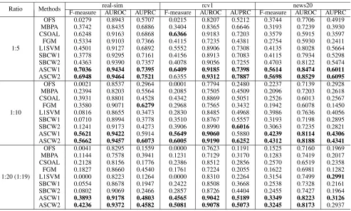
Test Performance.We report the test performances of all algorithms under different imbalance ratios in Table 3. It is observed that ASCW outperforms all other algorithms on most settings for the three performance measures. Also, the improvements of ASCW on F-measure are higher than that on AUROC and AUPRC.

(7)

Table 3: Average test performance over models trained on 20 random data permutations

Ratio Methods real-sim rcv1 news20

F-measure AUROC AUPRC F-measure AUROC AUPRC F-measure AUROC AUPRC

1:5

OFS 0.0279 0.8943 0.5707 0.0215 0.8207 0.5212 0.3744 0.7706 0.4919 MBPA 0.3742 0.8435 0.6886 0.3404 0.8365 0.6646 0.3193 0.7239 0.3930 CSOAL 0.6248 0.9163 0.6868 0.6366 0.9183 0.7203 0.3579 0.5915 0.3597 FGM 0.5334 0.9103 0.7366 0.4115 0.7235 0.4381 0.2754 0.5930 0.2411 L1SVM 0.4501 0.9127 0.6892 0.5552 0.8906 0.7308 0.4135 0.8028 0.5664 SBCW1 0.3778 0.9295 0.7161 0.4156 0.8913 0.7083 0.4115 0.7934 0.5298 SBCW2 0.4363 0.9390 0.7357 0.4078 0.9056 0.7255 0.4703 0.8122 0.5474 ASCW1 0.7036 0.9434 0.7395 0.6409 0.9185 0.7398 0.5614 0.8474 0.6011

ASCW2 0.6948 0.9464 0.7521 0.6355 0.9312 0.7887 0.5698 0.8529 0.6095

1:10

OFS 0.0021 0.8537 0.2964 0.0001 0.7794 0.2480 0.2237 0.7139 0.2928 MBPA 0.2394 0.8203 0.5564 0.2085 0.7505 0.4509 0.2096 0.7203 0.2618 CSOAL 0.3931 0.8801 0.4528 0.4342 0.8869 0.5051 0.2526 0.6013 0.2567 FGM 0.3580 0.9071 0.6279 0.2968 0.7565 0.3432 0.1942 0.6078 0.1450 L1SVM 0.0816 0.8655 0.3473 0.2830 0.8485 0.4968 0.3986 0.7636 0.4056 SBCW1 0.0710 0.8994 0.3778 0.3510 0.8767 0.5557 0.3193 0.7198 0.2895 SBCW2 0.1241 0.9173 0.4273 0.3906 0.8990 0.6016 0.3063 0.7235 0.2821 ASCW1 0.5621 0.9422 0.5914 0.5649 0.9060 0.5880 0.4239 0.8114 0.4306

ASCW2 0.5662 0.9457 0.6073 0.6005 0.9190 0.6252 0.4312 0.8188 0.4341

1:20 (1:19)

OFS 0.0041 0.8295 0.1559 0.0000 0.7623 0.1191 0.1525 0.7160 0.1969 MBPA 0.1144 0.7578 0.3941 0.1231 0.7129 0.3170 0.1283 0.7419 0.2017 CSOAL 0.2128 0.8156 0.1776 0.2386 0.8512 0.2856 0.2570 0.6519 0.2358 FGM 0.1827 0.8660 0.4540 0.1761 0.7224 0.2055 0.1622 0.6981 0.1282 L1SVM 0.0000 0.8223 0.1264 0.0000 0.8310 0.2264 0.3154 0.7499 0.2991

SBCW1 0.0554 0.8678 0.1947 0.2422 0.8508 0.3668 0.2538 0.7328 0.2161 SBCW2 0.0802 0.9069 0.2466 0.2857 0.8726 0.4404 0.2455 0.7427 0.1964 ASCW1 0.3893 0.9178 0.4803 0.4565 0.9042 0.5189 0.3349 0.8223 0.3126

ASCW2 0.4236 0.9372 0.4582 0.5081 0.9078 0.5073 0.3245 0.8173 0.2937

Table 4: Average estimated error of costˆc+by Algorithm 2 and optimal costc∗+.

Ratio Methods real-sim rcv1 news20

F-measure AUROC AUPRC F-measure AUROC AUPRC F-measure AUROC AUPRC

1:5 ASCW1 0.0008 0.0000 0.0000 0.0090 0.0032 0.0021 0.0073 0.0058 0.0140 ASCW2 0.0056 0.0031 0.0078 0.0082 0.0208 0.0345 0.0198 0.0020 0.0103

1:10 ASCW1 0.0000 0.0006 0.0014 0.0014 0.0084 0.0201 0.0006 0.0017 0.0119 ASCW2 0.0071 0.0006 0.0040 0.0111 0.0235 0.0117 0.0033 0.0069 0.0233

1:20 (1:19) ASCW1 0.0000 0.0000 0.0000 0.0542 0.0076 0.0354 0.0069 0.0024 0.0089 ASCW2 0.0000 0.0023 0.0011 0.0357 0.0345 0.0501 0.0107 0.0019 0.0148

ASCW to two main reasons. First, our algorithm is capable of selecting a close-to-optimal cost vector[c+, c−], which

makes it perform better on imbalanced measures. Moreover, there is a theoretical guarantee on the lower bound of F-measure. It explains the higher improvements of F-measure compared with AURROC and AUPRC. Second, our algo-rithm employs covariance structure that can better capture the interplays among features to find more effective features.

6.4 Optimal Cost Vector

In preposition 1, we theoretically analyze the lower-bound of the F-measure achieved by Algorithm 2. In order to quan-titatively verify that our algorithm can choose near to op-timal cost vector [c+, c−], we perform cost-sensitive

fea-ture selection by Algorithm 1 with costs vary amongc+ =

{0.55,0.60, . . . ,0.95} and choose the best cost according to overall online performance, denoted byc∗₊. To compare our selected cost with the best performance cost, we average

c+sampled in Algorithm 2 in the last 20 iterations (>5000

examples) as an estimation of the best cost, denoted asˆc+.

Then we compute the estimated errors as: |c∗₊−ˆc+| and

present the results on Table 4. We can observe that the es-timated errors of our algorithm and the optimal one is very close with the search length of0.05, thus verifying the accu-rate estimation of our algorithm for the optimal cost.

7 Conclusion

(8)

the best performance for prediction. We theoretically en-hance the theory of the existing sparse CW feature selection algorithm and analyze the performance behavior regarding F-measure. Experimental results show the superior perfor-mance of ASCW and its ability for selecting the satisfactory cost vector.

Acknowledgments

Yanbin Liu, Yan Yan, Ling Chen and Yi Yang are in part sup-ported by Data to Decisions CRC (D2D CRC). Yahong Han is in part supported by the NSFC (under Grant U1509206, 61472276, 61876130).

References

Crammer, K.; Dekel, O.; Keshet, J.; Shalev-Shwartz, S.; and Singer, Y. 2006. Online passive-aggressive algorithms. Journal of Machine Learning Research7(Mar):551–585.

Crammer, K.; Dredze, M.; and Pereira, F. 2009. Exact convex confidence-weighted learning. InAdvances in Neural Information Processing Systems, 345–352.

Crammer, K.; Kulesza, A.; and Dredze, M. 2009. Adaptive reg-ularization of weight vectors. InAdvances in neural information processing systems, 414–422.

Dong, X.; Yan, Y.; Tan, M.; Yang, Y.; and Tsang, I. W. 2019. Late fusion via subspace search with consistency preservation. IEEE Transactions on Image Processing28(1):518–528.

Han, C.; Tan, Y.-K.; Zhu, J.-H.; Guo, Y.; Chen, J.; and Wu, Q.-Y. 2016. Online feature selection of class imbalance via pa algorithm.

Journal of Computer Science and Technology31(4):673–682. Hoi, S. C.; Wang, J.; and Zhao, P. 2014. Libol: A library for online learning algorithms. The Journal of Machine Learning Research

15(1):495–499.

Kortanek, K. O., and No, H. 1993. A central cutting plane al-gorithm for convex semi-infinite programming problems. SIAM Journal on optimization3(4):901–918.

Ma, J.; Saul, L. K.; Savage, S.; and Voelker, G. M. 2009. Identi-fying suspicious urls: an application of large-scale online learning. InProceedings of the 26th annual international conference on ma-chine learning, 681–688. ACM.

Ma, J.; Kulesza, A.; Dredze, M.; Crammer, K.; Saul, L.; and Pereira, F. 2010. Exploiting feature covariance in high-dimensional online learning. InProceedings of the Thirteenth International Conference on Artificial Intelligence and Statistics, 493–500. Martins, A. F. T.; Smith, N.; Xing, E.; Aguiar, P.; and Figueiredo, M. 2011. Online learning of structured predictors with multiple kernels. InProceedings of the Fourteenth International Conference on Artificial Intelligence and Statistics, 507–515.

Rosenblatt, F. 1958. The perceptron: a probabilistic model for information storage and organization in the brain. Psychological review65(6):386.

Sahoo, D.; Hoi, S.; and Zhao, P. 2016. Cost sensitive online multi-ple kernel classification. InAsian Conference on Machine Learn-ing, 65–80.

Shalev-Shwartz, S., and Zhang, T. 2014. Accelerated proximal stochastic dual coordinate ascent for regularized loss minimization. InInternational Conference on Machine Learning, 64–72. Sumita, H.; Kawase, Y.; Fujita, S.; Fukunaga, T.; and Center, R. A. 2017. Online optimization of video-ad allocation. In Proceed-ings of the 26th International Joint Conference on Artificial Intel-ligence, 423–429. AAAI Press.

Tan, M.; Yan, Y.; Wang, L.; Van Den Hengel, A.; Tsang, I. W.; and Shi, Q. J. 2016. Learning sparse confidence-weighted classifier on very high dimensional data. InAAAI, 2080–2086.

Tan, M.; Tsang, I. W.; and Wang, L. 2014. Towards ultrahigh dimensional feature selection for big data.The Journal of Machine Learning Research15(1):1371–1429.

Tan, M.; Wang, L.; and Tsang, I. W. 2010. Learning sparse svm for feature selection on very high dimensional datasets. InProceedings of the 27th international conference on machine learning (ICML-10), 1047–1054.

Wang, J.; Zhao, P.; Hoi, S. C.; and Jin, R. 2014. Online feature selection and its applications. IEEE Transactions on Knowledge and Data Engineering26(3):698–710.

Wang, J.; Zhao, P.; and Hoi, S. C. 2012. Exact soft confidence-weighted learning. InProceedings of the 29th International Cofer-ence on International ConferCofer-ence on Machine Learning, 107–114. Omnipress.

Wang, J.; Zhao, P.; and Hoi, S. C. 2014. Cost-sensitive online clas-sification.IEEE Transactions on Knowledge and Data Engineering

26(10):2425–2438.

Wu, X.; Yu, K.; Ding, W.; Wang, H.; and Zhu, X. 2013. Online feature selection with streaming features. IEEE transactions on pattern analysis and machine intelligence35(5):1178–1192. Wu, Y.; Hoi, S. C.; Mei, T.; and Yu, N. 2017. Large-scale online feature selection for ultra-high dimensional sparse data.

ACM Transactions on Knowledge Discovery from Data (TKDD)

11(4):48.

Yan, Y.; Yang, T.; Yang, Y.; and Chen, J. 2017. A framework of online learning with imbalanced streaming data. InAAAI, 2817– 2823.

Yu, K.; Wu, X.; Ding, W.; and Pei, J. 2014. Towards scalable and accurate online feature selection for big data. InData Mining (ICDM), 2014 IEEE International Conference on, 660–669. IEEE. Yuan, G.-X.; Chang, K.-W.; Hsieh, C.-J.; and Lin, C.-J. 2010. A comparison of optimization methods and software for large-scale l1-regularized linear classification. Journal of Machine Learning Research11(Nov):3183–3234.

Zhao, P., and Hoi, S. C. 2013. Cost-sensitive online active learning with application to malicious url detection. InProceedings of the 19th ACM SIGKDD international conference on Knowledge dis-covery and data mining, 919–927. ACM.

Zhao, P.; Zhang, Y.; Wu, M.; Hoi, S. C.; Tan, M.; and Huang, J. 2018. Adaptive cost-sensitive online classification.IEEE Transac-tions on Knowledge and Data Engineering.

Zhou, P.; Hu, X.; Li, P.; and Wu, X. 2017. Online feature se-lection for high-dimensional class-imbalanced data. Knowledge-Based Systems136:187–199.