Efficient Data Dependence Profiling.

(1)

Abstract

VANKA, RAJESHWAR. Efficient Data Dependence Profiling. (Under the direction of James Tuck.)

With processor frequencies leveling off and core designs remaining relatively static, optimiz-ing existoptimiz-ing software to achieve higher performance is increasoptimiz-ingly important. Prior works have shown that speculating on conservative data dependence constraints can unlock performance potential within existing codes. Techniques such as thread-level speculation and speculative optimizations leverage this property to perform risky transformations to boost performance. In order to maximize the potential of these techniques, accurate knowledge of the data depen-dences in question is necessary. Data dependence profilers (DDPs) provide this information by tracking dependences during execution using representative inputs.

In this thesis, I’ll first describe and evaluate a conventional data dependence profiler, and expose its shortcomings. Traditional profilers use a centralized structure to track dependences. This leads to slow and inaccurate profiling. Subsequently, I’ll introduce a novel set-based profil-ing scheme which uses sets to provide decentralized storage and operations. The scheme utilizes static analysis to precisely identify the dependences that need to be tracked, and performs a greedy set allocation to group the instructions (and hence dependences) across sets.

Software signatures (simple bloom filters) are used to realize the sets at runtime. The signa-tures are highly tunable, and provide quick, albeit imprecise, operations. Using these operations, we are able to track dependences at runtime. With the help of smart optimizations, the scheme can profile large programs quickly and accurately. Significantly, tests show that the performance (slowdown versus uninstrumented code) of the profiler can be significantly improved without necessarily sacrificing accuracy.

The profiler is evaluated using queries from a Speculative Code Motion pass. The pass identifies scheduling opportunities involving loads and prior stores which might share the same address. These queries cover (on average) >80% of the memory operations in the SPEC2000 suite of programs. The profiler is able to collect the necessary information with an overhead of 100%, with an accuracy of 0.19 NAED (Normalized Average Euclidean Distance). This compares with an accuracy of 0.40 NAED achieved by a traditional DDP with larger overheads. The profiler achieves this accuracy with ¡ 100% overhead versus an aggressively optimized uninstrumented baseline.

(2)

profile data, and its effect on these optimizations are analyzed. We show that there is untapped performance within existing programs that can realized through speculative optimizations, and that data dependence profiling can deliver performance improvements. Using the set-based profiler scheme, a 4.4% improvement in dynamic instruction count is realized, leading to a 5% improvement in execution time. In equake, we see a 20% improvement in instruction count, leading to a>10% improvement in cycles across all configurations. Further experiments showed that these results closely match the opportunity found using an ideal profiler. This shows that the set-based profiler is accurate enough to realize almost all of the opportunity available.

(3)

(4)

Efficient Data Dependence Profiling

by

Rajeshwar Vanka

A dissertation submitted to the Graduate Faculty of North Carolina State University

in partial fulfillment of the requirements for the Degree of

Doctor of Philosophy

Computer Engineering

Raleigh, North Carolina 2013

APPROVED BY:

Xiaosong Ma Eric Rotenberg

Huiyang Zhou James Tuck

(5)

Dedication

(6)

Biography

The author was born in Hyderabad, the capital of the state of Andhra Pradesh situated on the Deccan Plateau in south India. His parents, Dr. V. S. S. Sastry and Dr. N. Satyavathi, are natives of Andhra Pradesh as well. Dr. Sastry works as a physics professor in University of Hyderabad, whereas his mom, Dr. Satyavathi, worked as a physics professor in Osmania University. His brother, Dr. Sundaram Vanka, works in field of wireless networks and recently completed his PhD from the University of Notre Dame.

(7)

Acknowledgements

I come from an academic family, with both my parents working as physics professors. My brother recently completed a PhD in wireless networks. This background provided an excellent foundation for pursuing graduate studies and proceeding towards research. I’m very grateful to my family for providing me with the analytical skills and nurturing interest in the field of my choice. I was inspired to pursue this degree after witnessing their understanding and excitement with their respective areas.

Upon completion of my bachelors degree, I traveled to the US and was met by Sridhar Kudumala and his wife, Kavita. They helped me make the transition and set myself up in Raleigh. I would like to thank them for their help and hospitality.

I met with Dr. James Tuck prior to the first day of classes, and have been interacting with him ever since. He has been the single biggest influence in my career over the past few years, and I’m very much grateful to him for his advise, patience and resolve to ensure that I understood the ins and outs of research, and to place knowledge of the subject above all other considerations. My background in compilers was weak, at best, when I started out at NCSU. I’m deeply grateful for his mentoring, and for showing how to understand and navigate the field. Besides my family, he has been the single biggest influence on my career, and I’m pleased to continue working with him after the completion of the degree.

I would like to thank the thesis committee for their insight comments and suggestions. I have interacted with Dr. Huiyang Zhou and Dr. Xiaosong Ma when I took their courses on GPUs and distributed systems. I believe that understanding a field requires breadth. Their courses, and more importantly, their presence on the thesis committee has been very helpful in this regard. My association with Dr. Rotenberg goes back to Fall 2008, when I was assigned as a teaching assistant for his course on computer architecture. Subsequently, I took his course on advanced microarchitecture, and worked as a teaching assistant for that course. During these times, I have had the chance to interact with him and his group. I admire the clarity in his arguments, and his attention to detail which often exposes interesting observations. It was a pleasure working with him, as my understanding of the subject matter got better each time.

(8)

stay at the lab memorable.

Finally, I would like to thank the friends that have made my time at NC State memorable. I would like to thank my roommates and good friends, Sankararaman Janakiraman, Rajeev Patwari, Rajsekhar Santhapoor and Salil Wadhavkar, with whom I shared many good times. The chilly winter vacations, and the deserted summers were more fun thanks to all the hangouts and potlucks.

The CESR lab was a vibrant place, and I made many good friends over the course of my stay. In alphabetical order, they are Siddhartha Chhabra, Niket Choudhry, Sabina Grover, Saurabh Gupta, Sandeep Navada, Poulomi Pal, Salil Pant and Devesh Tiwari. Devesh’s name comes at the end of the list, but he was the first person I met in the lab, and has been a very good friend ever since. I’m very happy that I had the opportunity to share fruitful discussions, and late night chats with them.

My intenship at Dr. Quinlan’s group was memorable, and part of the credit goes to the other interns and my relatives in California who made me feel at home. My uncle, Satya Nish-tala and his wife, Seetha are my second family now. Their son, Rajesh NishNish-tala and his wife, Rakhee provided the support necessary to enjoy the time. At the lab itself, I made quite a few friends, and I cherish them even today. In alphabetical order, they are Sriram Ananthakrish-nan, Akshatha Bhat, Pei-Hung Lin, Hongyi Ma, Steena Monteiro and Tristan Vanderbruggen. Interestingly, Akshatha and myself joined the same company, and share many stories from the internship times.

Finally, there are a few friends whom I met informally, and the friendships have blossomed over the years. I would like to thank Santosh Navada and Shivam Priyadarshi for their support and encouragement when the times were tough. Halley Tej, Arjun Bangre and Karteek Peri were the first few friends I made at NC State, and I owe them a great deal for helping me settle down in this place. I cherish their friendship, and would like to acknowledge their role in achieving this milestone.

Finally, I would like to especially thank Aishwarya Ramaswamy who has been a friend for more than a decade now, and has been a constant source of humor, laughter and a dose of reality. She is a constant reminder of the life outside the world of engineering.

(9)

Table of Contents

List of Tables . . . ix

List of Figures . . . x

Chapter 1 Introduction . . . 1

1.1 Data Dependence Profiling . . . 1

1.2 Traditional Data Dependence Profilers . . . 2

1.2.1 Operation . . . 2

1.3 Set-based Profiling using Software Signatures . . . 3

1.3.1 Signatures . . . 4

1.4 Feedback Directed Optimizations . . . 4

Chapter 2 Background. . . 5

2.1 Alias analysis - data dependences . . . 5

2.2 Bloom filters and Software Signatures . . . 9

2.3 Signature Operations . . . 10

Chapter 3 Methodology . . . 13

3.1 Host System and Benchmarks . . . 13

3.2 Compiler . . . 13

3.2.1 Data Dependence Profilers . . . 15

3.2.2 Feedback Directed Optimization . . . 15

3.3 Speculative Code Motion . . . 18

3.4 Sampling . . . 19

3.5 Performance and Accuracy Metrics . . . 19

Chapter 4 Traditional Data Dependence Profilers . . . 21

4.1 Design . . . 21

4.1.1 Original Design . . . 21

4.1.2 Streamlined Design . . . 22

4.1.3 Improved Original Design . . . 23

4.2 Evaluation . . . 23

4.3 Drawbacks . . . 31

4.3.1 Original Design . . . 31

Chapter 5 Set-based Profiling using Software Signatures . . . 33

5.1 Main Idea . . . 33

5.2 Set-Based Profiler Design . . . 34

(10)

5.2.2 Set Allocation . . . 38

5.2.3 Instrumentation . . . 39

5.2.4 Root Sets with Membership . . . 40

5.3.1 Experimental Setup . . . 43

5.3.2 Performance and Accuracy . . . 43

5.3.3 Quality of Accuracy . . . 44

5.3.4 Set Operations Counts . . . 45

5.3.5 Signature Sizing . . . 49

5.3.6 Effect of Sampling . . . 51

5.3.7 Single Array Signatures . . . 53

5.3.8 Hardware Signatures . . . 55

5.4 Summary . . . 57

Chapter 6 Optimizations to Set-based Profiling . . . 59

6.1 Motivation . . . 59

6.2 Early Termination . . . 60

6.2.1 Set Profiler . . . 60

6.2.2 Results . . . 61

6.2.3 Summary . . . 63

6.3 Set Customization Using Edge Profiling . . . 64

6.3.1 Estimating Population Using Edge Profiling . . . 64

6.3.2 Set Customization . . . 65

6.3.3 Results . . . 66

6.4 Improving Accuracy Using Better Set Allocation . . . 66

6.4.1 Static Insertion Counting . . . 68

6.4.2 Characterization . . . 71

6.5.1 Comparison with Prior Set Profiler Configurations . . . 74

6.5.2 Improving Traditional Profilers using Sets . . . 78

6.6 Summary . . . 82

Chapter 7 Feeding back Data Dependence Profile Information . . . 83

7.1 Feeding back profile information . . . 83

7.1.1 Running Example . . . 84

7.1.2 Edge Profile Feedback . . . 85

7.1.3 Data Dependence Profile . . . 88

7.2.1 Setup . . . 91

7.2.2 Edge Profile . . . 94

7.2.3 Edge and Data Dependence Profile . . . 96

7.2.4 Comparison with Traditional Profilers . . . 99

7.2.5 Comparison with Ideal Profiler . . . 103

(11)

Chapter 8 Related Work . . . .107

8.2 Speculative Optimizations . . . 108

Chapter 9 Conclusion . . . .110

9.2 Feedback Directed Optimization . . . 111

References. . . .113

Appendix . . . .117

Appendix A Tool Description . . . 118

A.1 Profiler . . . 119

(12)

List of Tables

Table 3.1 Processor Configurations . . . 14

Table 3.2 Profile Coverage - Loads and Stores profiled . . . 18

Table 4.1 Changes in design to streamline the profiler . . . 23

Table 5.1 Profiler Configurations . . . 42

Table 5.2 Accuracy and its impact . . . 45

Table 6.1 Characterization of Baseline Profiler. . . 60

Table 6.2 System Configurations for Early Termination (ET). . . 61

Table 6.3 Effect of Early Termination on Conflict Checks . . . 63

Table 6.4 Population Distribution Percentage . . . 65

Table 6.5 Set Customization Types . . . 65

Table 6.6 System Configurations for Set Customization. . . 66

Table 6.7 Percentage Increase in Sets of Each Type . . . 68

Table 6.8 System Configurations for new Population-Based Set Allocation. . . 69

Table 6.9 Original Set Distribution . . . 71

Table 6.10 AllocS Set Distribution . . . 72

Table 6.11 Percentage change in Set Distribution . . . 72

Table 7.1 Processor Configurations . . . 91

(13)

List of Figures

Figure 1.1 An example of data dependence profiling. . . 3

Figure 2.1 An example CFG for a function. . . 6

Figure 2.2 Responses from Alias Analysis . . . 7

Figure 2.3 Runtime information gathered by a data dependence profiler . . . 7

Figure 2.4 Profile Data classification and transformation . . . 8

Figure 3.1 Typical workflow in LLVM . . . 14

Figure 3.2 Workflow with Data Dependence Profile . . . 14

Figure 3.3 Workflow with Edge Profile feedback . . . 15

Figure 3.4 Workflow with DDP and Edge Profile feedback to FDO . . . 16

Figure 3.5 Examples of dependence checks for speculative optimizations. . . 17

Figure 3.6 Figure showing variation of NAED in different scenarios . . . 20

Figure 4.1 Impact of size on Streamlined Hash Tables . . . 24

Figure 4.2 Impact of sampling on Streamlined Hash Tables with 50000 entries . . . . 26

Figure 4.3 Impact of sampling on Streamlined Hash Tables with 100000 entries . . . 27

Figure 4.4 Impact of sampling on Streamlined Hash Tables with 200000 entries . . . 28

Figure 4.5 Tagged Hash Tables with 20 Tags per entry . . . 29

Figure 4.6 Tagged Hash Tables with 10 Tags per entry . . . 30

Figure 5.1 Examples of dependence checks for speculative optimizations. . . 34

Figure 5.2 Stages in Set-based Profiler . . . 35

Figure 5.3 Interference Graph using proposed set allocation schemes. . . 37

Figure 5.4 Allocating QSets to PSets using Interference Graph . . . 39

Figure 5.5 Instrumentation using Disambiguation . . . 41

Figure 5.6 Instrumentation using Membership . . . 41

Figure 5.7 Performance and accuracy comparison of best signature and best hash table designs. . . 43

Figure 5.8 Set Characterization Part 1 . . . 46

Figure 5.9 Set Characterization Part 2 . . . 47

Figure 5.10 Performance and accuracy comparison of signature designs . . . 50

Figure 5.11 Performance and accuracy variation for S RM 2K using different sample rates . . . 52

Figure 5.12 Performance and accuracy comparison of single array signature designs . . 54

Figure 5.13 Impact on SpecLICM - Percent of Insts and Loads Moved . . . 56

Figure 5.14 HW Cache Hit Percentage . . . 57

Figure 6.1 Early Termination . . . 62

Figure 6.2 Early Termination + Set Customization . . . 67

Figure 6.3 Early Termination + Set Allocation Using Static Insertion Counting . . . 70

(14)

Figure 6.5 Early Termination + Set Customization + Set Allocation Using Static

Insertion Counting . . . 73

Figure 6.6 Fractional changes in Membership Counts . . . 74

Figure 6.7 Fractional Decreases in Insertion and Membership Counts With Sampling 75 Figure 6.8 Fractional Decreases in Insertion and Membership Counts With Sampling 76 Figure 6.9 Comparison with Prior Configurations . . . 77

Figure 6.10 Effect on Speculative LICM . . . 78

Figure 6.11 Traditional Profilers using Sets . . . 79

Figure 6.12 Traditional Profilers using Sets with Sample Rate 10 . . . 80

Figure 6.13 Traditional Profilers using Sets with Sample Rate 100 . . . 81

Figure 7.1 An example code . . . 84

Figure 7.2 An example code . . . 86

Figure 7.3 Impact on code . . . 86

Figure 7.4 Applying basic block straightening impacted code . . . 86

Figure 7.5 No Aliases . . . 89

Figure 7.7 Must Aliases . . . 90

Figure 7.9 Workflow with DDP and Edge Profile feedback to FDO . . . 92

Figure 7.10 Speedup in IPC using Config E . . . 94

Figure 7.11 Percentage Improvement using Config E . . . 95

Figure 7.12 Speedup in IPC using Config EN-S . . . 97

Figure 7.13 Percentage Improvement using Config EN-S . . . 98

Figure 7.14 IPC improvement using Config ENM-S instead of E . . . 99

Figure 7.15 Percentage improvement using Config ENM-S instead of E . . . 100

Figure 7.16 Performance improvement using Config ENM-S over B . . . 101

Figure 7.17 Performance improvement when using Config ENM-S instead of ENM-T . 102 Figure 7.18 Performance improvement using Config EN-I over EN-S . . . 104

Figure A.1 Code Layout for Profiling . . . 119

(15)

Chapter 1

Introduction

1.1 Data Dependence Profiling

Programs are written such that they can handle a multitude of inputs, that exercise a large number of control and data flow paths within the code. Studies have shown that certain paths (control and data) are exercised far more than others. These paths are commonly called hot

paths. Compilers which translate these programs into efficient, semantically correct machine

code have to account for all the paths within the code, and hence generate code that is frequently sub-optimal in the common case. Speculative optimizations aggressively transform the code by performing risky transformations which are only valid under certain inputs. By optimizing the code for the common case, the resulting code runs faster, most of the time. Monitoring and recovery support ensures that the semantics of the program are never violated. These optimizations can work better if they are provided with runtime information regarding the behavior of the code. In order to continue delivering performance improvements in static and dynamic compilation environments, gathering runtime information quickly and accurately is becoming increasingly important. Profiling is a way of gathering such information.

Edge profiling determines the probability that a given control flow edge (an edge connecting two basic blocks in a program) is taken. This information helps the compiler bias its decisions towards the more frequently taken path. Data dependence profiling determines the probability that a given data flow edge (an edge connecting two memory operations) occurs. This allows the compiler to optimize the code surrounding the instructions better. As an example, an invariant load that doesn’t have a data flow edge to any other stores in a loop, can be hoisted from the loop. In addition to the load, its slice is now eligible for hoisting as well.

(16)

on VLIW processors and speculative loop parallelization techniques have shown that data de-pendence profiling can help unlock performance hidden within existing codes. Therefore, in this thesis, we describe a new set-based data dependence profiling technique that is both faster and more accurate than prior works.

The need for data dependence profiling arises from the transformations that optimizations try to perform, but are unable to, due to conservative alias analyses. Prior works have designed data dependence profilers that can collect runtime information for entire programs. However, in our studies, we show that these profilers are either too slow, inaccurate or cannot capture certain relationships within the program at all. We describe the design of these profilers in the next section. The reader may find a more detailed study of these profilers in Chapter 4.

1.2 Traditional Data Dependence Profilers

As mentioned previously, prior works [9, 12, 24] have proposed data dependence profilers. These profilers have many similarities, hence we refer to them astraditional data dependence profilers. We base our discussion here on [9], which best describes their design.

These profilers use a centralized structure, typically with functionality similar to that of a hash table, to record the dependence information for a given region. In most cases, the region refers to the entire program, however it can be tailored to work with functions or loops. The structure(s) is(are) designed such that instructions accessing the same location are recorded as dependence chains. In a typical design, consecutive entries in the dependence chain refer to consecutive instructions that access the same location in memory. In order to form these dependence chains at runtime, all instructions refering to a given memory location share an entry in the structure. Each time an instruction needs to access the structure, it uses the address (its accessing in memory) to lookup the entry in the table. Hence, in order to form the dependence chains accurately, the size of the structure should be equal to number of unique addresses accessed by the program. This is an exorbitant cost, and clearly not scalable to large programs. For this reason, most techniques restrict the size of the table, which paves the way for false dependences to creep into the chains.

1.2.1 Operation

(17)

(1) store A (2) store B

(8) load X (9) load Y

(1) store A profSt(A,1) (2) store B profSt(B,2)

(8) load X profLd(X,8) (9) load Y profLd(Y,9)

(a) (b)

X

B

A 1

8

2

(9) Y

(c)

13

X 8

B 2 A 1

(9) Y

Hash Table Fixed Table Annotated Code

Code

(d)

Dep. Edge 2->9 Dep. Edge 2->9

Figure 1.1: An example of data dependence profiling.

Such structures may be fixed-size tables or large and virtually unlimited hash tables. In most medium-to-large programs, a fixed-size table is necessary as infinite size hash tables quickly consume all available memory. Parts (c) and (d) show an insertion operation. At load Y, the table is indexed using the address (Y), which clashes with an entry for address B (entered at store B) in the table. A dependence between 9 (current instruction) and 2 (prior instruction) is recorded. Instruction 9 then replaces 2 as the most recent instruction to that index.

Given a fixed-size table design, like Part(d), it is possible that B and A share the same entry in the hash table. In this case, a false dependence between instructions 9 and 1 would be recorded. Even with proper calculation of the dependence chains, this design does not provide accurate answers required by optimizations, to speculatively transform the code. This profiler design is described in greater detail, and evaluated in Chapter 4.

1.3 Set-based Profiling using Software Signatures

In order to overcome the problems with existing DDPs, we took a fundamentally different ap-proach to calculating dependences. Instead of using a single structure, and tracking dependences in chains, we use a decentralized/distributed storage to track runtime dependences. We call this distributed storage, sets. Using static analysis, we are able to figure out which instructions are likely to conflict (i.e. have the same address). Hence, we can use the sets as runtime storage of

theaddresses of these instructionsand use set operationsto figure out if there are any conflicts

(18)

we can design storage for each group of instructions that are likely to conflict with one another. We find such group of instructions using set formation, and subsequently allocate sets using novel set allocation techniques. Briefly, we record relevant queries either through heuristics or from optimizations. The relationships between these queries are analyzed, and a greedy set allocation scheme quickly assigns storage in the form of sets. Based on this set allocation, set operations are chosen.

1.3.1 Signatures

The set operations that we use here include insertion, disambiguation and membership check. These operations can be quickly performed at runtime using software/hardware signatures. We evaluate our profiler using software signatures (simplified bloom filters) and a hardware signature cache. Signatures provide concise and imprecise storage for the sets. We show that through smart allocation schemes, the imprecision can be limited without necessarily sacrificing performance.

1.4 Feedback Directed Optimizations

(19)

Chapter 2

Background

This chapter provides background information which is helpful in understanding the later chap-ters. An basic introduction to alias analyses and their relation to data dependence profiling is provided. Subsequently, bloom filters and signatures are discussed. The set-based profiler relies on software signatures to realize set operations at runtime.

2.1 Alias analysis - data dependences

Alias analysis tries to determine if two or more memory operations can ever access the same address at runtime. In other words, alias analysis tries to determine if the address operands in each of the instructions are always equal, i.e. aliases. Using static analysis, alias analyses typically provide one of the three following answers.

• The instructions in question do not alias, refered to asno-alias

(20)

1. LD BR B2, B3

2. ST BR B4

3. ST BR B4

4. LD BR B5, B6

5. LD BR B6

6. ST RET

ENTRY

B2 B3

B4

B5

B6

EXAMPLE CFG WITH MEM OPS

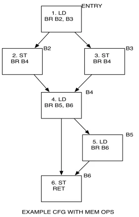
Figure 2.1: An example CFG for a function.

The may-alias response means that the alias analysis is not able to ascertain a definite

relationship between the instructions in question. A data dependence profile can quantify the relationship between the two instructions, by calculating the probability that the instructions in question share a dependence. This information is valuable to optimizations which can now optimize the code, albeit with speculative information. The profiling information is speculative since it is only valid for the given inputs, and even on other correlated inputs, the behavior might be vary on occasion. Hence, any transformations using data dependence profiling are speculative. In case of SpeculativePRE [33], this speculation may not result in loss of semantics, but a loss of performance.

(21)

1. LD

2. ST 3. ST

4. LD

5. LD

6. ST

MAY ALIAS REL ALIAS ANALYSIS RESULTS

Figure 2.2: Responses from Alias Analysis

1. LD

2. ST 3. ST

4. LD

5. LD

6. ST

A 0xFD

B 0xDF

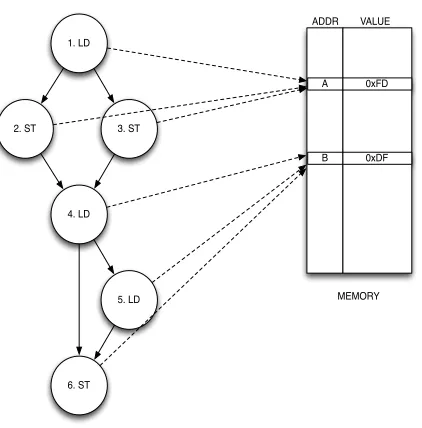
DDP DATA REPRESENTATION

MEMORY ADDR VALUE

(22)

1. LD

2. ST 3. ST

4. LD

5. LD

6. ST

1. LD 8. LD

2. ST 3. ST

7. ST 4. LD

5. LD

6. ST

(a) (b)

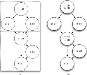
Figure 2.4: Profile Data classification and transformation

8

(23)

the stores 2 and 3. Since load 4 and load 5 access the same address without an intervening store, load 5 is redundant and hence removed. Therefore, in this example, DDP information was able to remove 3 memory operations.

Since the number of data dependences within even medium-sized programs are often quite large, smart strategies are required to quickly and accurately gather this runtime information. In Chapter4, we discuss how hash-table profilers try to solve this problem, and in Chapters 5 and 6, we describe how a novel set-based profiler efficiently profiles large programs.

2.2 Bloom filters and Software Signatures

We employ software signatures to perform the insertion, disambiguation and membership op-erations on the sets of instructions. Here, we describe the design of the software signatures, and their roots in hardware signatures and bloom filters.

Bloom filters [4] provide concise storage of data in a bit-vector while providing high accuracy for disambiguation and membership operations on the recorded data. Unlike other compression techniques, the inserted data cannot actually be retrieved, but rather can only be queried for existence. On such queries (intersection or membership), Bloom filters are able to answer with high accuracy whether that input was ever inserted in the filter. The answer is always conservative by design—it must answer yes if the data was ever inserted. If it answers no, then the data was never inserted. However, it may answer yes due to collisions even when the data is not present. Hence, Bloom filters suffer from false positives but not false negatives.

Bloom filters consist of one or more hash functions which are linked to a single/partitioned memory for storing data. The hash function(s) set bit(s) in the memory provided. Multiple hash functions provide resilience against false positives. Previous studies [15] have shown that using partitioned memory results in better performance versus accuracy tradeoffs in bloom filters.

Signatures are simplified bloom filters. They are essentially Bloom filters employing simpler hash functions and are tied to dedicated registers. In order to adapt them to hardware, the hash functions needed to be simplified, and the number of bits used were limited by the size of registers that can be feasibly implemented. These hardware derivations of bloom filters have been used in implementing memory consistency [6], memoization [29] and load-store queue disambiguation [27]. We found that these hardware signatures provide high accuracy on large sets of addresses, and since they were intended for hardware implementation, their runtime costs were low. For these reasons, we decided to implement them in software for the set-based profiler that we propose here. As our studies show, the software signatures provide a better tradeoff between accuracy and performance when compared to the current state-of-the-art hash table implementations.

(24)

Algorithms 1 through 3.

Algorithm 1:Insertion

Input: S: Signature is an{array of integer[M]}

Input: Addr: Data address

Result: Updated signature containing Addr.

1 h = Hash(Addr);

2 index = h/32;

3 bitpos = h mod 32;

4 S[index] = S[index]|(1bitpos);

5 returnS

Algorithm 2:Disambiguation

Input:S1: Signature{array of integer[M]} Input:S2: Signature{array of integer[M]}

Result: Boolean value indicating presence of conflict.

1 conflict=false;

2 fori=0; i<M; i++do

3 conflict = conflictk(S1[i]|S2[i] );

4 end

5 returnconflict

Algorithm 3:Membership Check

Input: S: Signature{array of integer[M]}

Input: Addr: Data address

Result: Boolean value indicating presence in S.

1 h = Hash(Addr);

2 index = h/32;

3 bitpos = h mod 32;

4 returnS[index] & (1bitpos)

2.3 Signature Operations

(25)

two sets. The membership operation checks if a single element is part of a set.

The accuracy and performance of signatures are important for the overall success of our set-based profiler. Since signature operations are imprecise, they may result in false positives. It is well known that keeping signatures relatively underpopulated for their size is important for attaining good accuracy, as shown in the following formula:

PN oConf lict∝

1− 1

# of bits in S kn

(2.1)

where n is the total size and k is a constant determined by the hashing function. We can understand the runtime costs by the following formula:

Overhead(S) = falloc(S)∗Nalloc

+finsert(S)∗Ninsert

+fdisamb(S)∗Ndisamb

+fmember(S)∗Nmember

+Nbloat (2.2)

wherefalloc(S),finsert(S),fdisambandfmemberare the costs of allocation, insertion, disambigua-tion and membership operadisambigua-tions on the signature, andNalloc,Ninsert,Ndisamband Nmember are their dynamic counts. Nbloat accounts for the deterioration in performance of the surrounding code due to optimization hurdles created by the signature. For signatures allocated on the stack,

falloc accounts for initialization costs.finsert and fmember are roughly equal in magnitude, and

vary depending on the size of the signature and hash functions used. fdisamb increases as the size of the signature increases. All dynamic counts are based on actual program behavior.

Membership vs. Disambiguation.

(26)

Signature Configuration

(27)

Chapter 3

Methodology

3.1 Host System and Benchmarks

The profilers were tested natively on an Intel Xeon two-way hyper-threaded quad-core machine with 6GB of RAM, and running RHEL 5. Eleven benchmarks from the SPEC2000 benchmark suite were used to evaluate the profilers. The fortran benchmarks in the suite were converted to C using f2c.

For the FDO framework, we simulated representative regions of the benchmarks (obtained through SESC [25] simulation marks), using PTLSim [35], a cycle-accurate x86 simulator. The

triggermechanism in PTLSim is used to select the regions identified by SESC simulation marks.

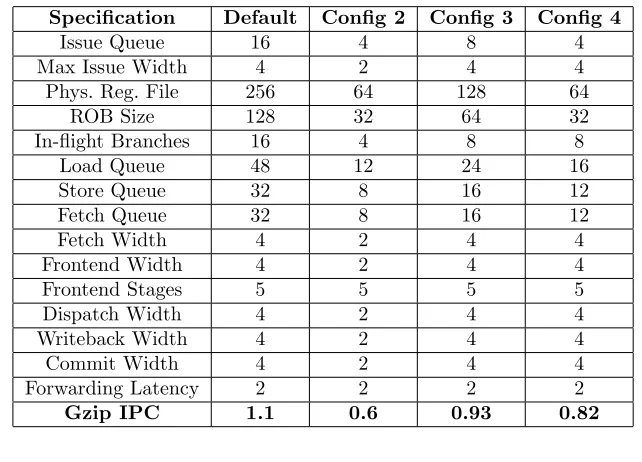
The processor configurations used for the PTLSim runs are listed in Table 7.1. The four config-urations listed are meant to represent various design points, with different levels of aggressive-ness in terms of structures and out-of-order behavior. The IPCs for the SPEC2000 benchmark, 164.gzip, are listed in the last row, as a reference. TheDefaultconfiguration is the most aggres-sive configuration, whereas Config 2 is the least aggressive. These configurations are used to understand the sensitivity of the feedback directed optimizations to the underlying hardware.

3.2 Compiler

The data dependence profilers are implemented as IR-level passes in LLVM 2.4 [19].

(28)

Table 3.1: Processor Configurations

Specification Default Config 2 Config 3 Config 4

Issue Queue 16 4 8 4

Max Issue Width 4 2 4 4

Phys. Reg. File 256 64 128 64

ROB Size 128 32 64 32

In-flight Branches 16 4 8 8

Load Queue 48 12 24 16

Store Queue 32 8 16 12

Fetch Queue 32 8 16 12

Fetch Width 4 2 4 4

Frontend Width 4 2 4 4

Frontend Stages 5 5 5 5

Dispatch Width 4 2 4 4

Writeback Width 4 2 4 4

Commit Width 4 2 4 4

Forwarding Latency 2 2 2 2

Gzip IPC 1.1 0.6 0.93 0.82

Alias Analysis LLVM

Bytecode

Optimizations (GVN, LICM,

PRE)

Optimized LLVM

Bytecode _Backend Optimized

Binary

Figure 3.1: Typical workflow in LLVM

Analysis (Speculative

Code Motion)

Interference Graph Generation

Set Allocation

Instrumen -tation LLVM

Bytecode

Queries Instrumented

LLVM Bytecode Set-based Profiler

(29)

LLVM Bytecode

Dead Block Elimination

Edge Profile Optimized

Bytecode

EDGE PROFILE DATA

Backend Optimized

Binary

Figure 3.3: Workflow with Edge Profile feedback

3.2.1 Data Dependence Profilers

The workflow for the data dependence profiler is described in Figure 3.2. The set-based profiler is implemented as a sequence of passes within LLVM, which operate at the IR-level. The output of these passes is instrumented bytecode. The passes provide a wide variety of instrumentation options which can be configured on the command line. The passes were invoked using the opt tool in LLVM.

The set-based profiler and the traditional (hash table) profiler are implemented as separate passes. We evaluate the impact of using the set allocation schemes on the hash table profiler as well. Each of the profilers uses the same bookkeeping code, to update counters to track aliases at runtime. Both the profilers output files in the same format, so a single feedback pass at the IR-level can understand the output of both the profilers.

Ideal Profiler This profiler calculates perfectly accurate profiles. Unlike the set-based or traditional profiler, this profiler does not lose precision. However, as a tradeoff, this profiler runs orders of magnitude slower than either of the two profilers evaluated here. This profiler was implemented as a gold standard for accuracy. It uses a large amount of memory to track runtime information, and couldn’t scale to some of the larger benchmarks, like gcc, and hence they were omitted from the results.

3.2.2 Feedback Directed Optimization

(30)

An a lysi s (Sp e cu la ti ve

Code _Moti

o n ) In te rf e re n ce G ra p h G e n e ra tio n Se t Al lo ca ti o n In st ru me n -tation Ed g e Pro fil e O p ti mi ze d Byt e co d e Q u e ri e s In st ru me n te d L LVM Byt e co d e Se t-b a se d Pro fil e r Ba cke n d In st ru me n te d Bi n a ry D A T A D EPEN D EN C E PR O F IL E D A T A EXEC U T E O N T R AI N I N PU T An a lysi s (Sp e cu la ti ve

Code _Moti

(31)

st A st B

ld X st C

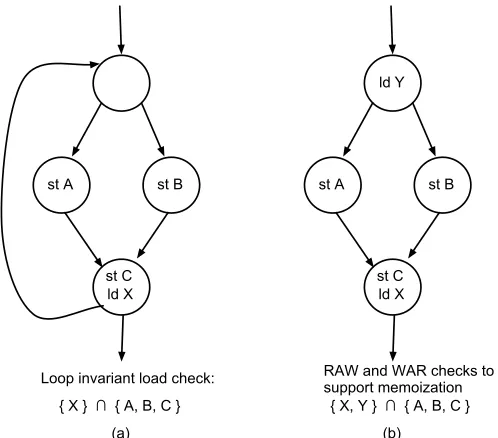
{ X } ∩ { A, B, C } (a)

Loop invariant load check:

st A st B

ld X st C ld Y

{ X, Y } ∩ { A, B, C } (b)

RAW and WAR checks to support memoization

Figure 3.6: Examples of dependence checks for speculative optimizations.

18

Figure 3.5: Examples of dependence checks for speculative optimizations.

version of LLVM uses the same techniques as the one in LLVM 2.4. In addition to the data dependence profiler, the edge profiler is incorporated in the tool, to provide runtime control-flow information. This information is used by the Dead Block Elimination pass to straighten the code, and remove unused blocks. This pass cleans up the code significantly. The workflow for the edge profile feedback is shown in Figure 3.3.

(32)

Table 3.2: Profile Coverage - Loads and Stores profiled Benchmarks %of Loads %of Stores %of F ns

gzip 79 80 62

swim 78 78 100

mgrid 79 60 100

applu 47 64 75

vpr 82 87 77

mesa 63 79 78

art 83 81 80

ammp 78 86 88

parser 84 90 77

bzip2 97 86 100

twolf 80 93 89

Average 77 80 84

3.3 Speculative Code Motion

Prior works on data dependence speculation have relied on Speculative Code Motion (SCM) to deliver performance improvements. SCM is an important optimization, since it can directly impact the execution time, as well as enable other optimizations to find more opportunity. Load re-ordering is an important part of SCM since increasing the scheduling freedom of loads allows slice instructions to enjoy the benefits as well. Figure 3.5 shows two examples where determining the relationship between a load and other stores within the function can enable LICM and memoization passes to find additional opportunity. In part(a), moving ld X out of the loop decreases its dynamic instruction count, and consequently allow LICM to find other invariant instructions. In part(b), if ld X doesn’t alias the other stores within the function, the function could be declared pure, and hence, memoizable. Performing these optimizations requires runtime information showing the likelihood of the relationships.

Algorithm 4:GenQueries

Input: P: Program being analyzed

Result: Relevant queries

1 foreach function∈Pdo

2 foreach load∈functiondo

3 foreach store that precedes load on some path do

4 if load may-aliases with storethen

5 Relevant query found. Mark for profiling.

6 end

7 end

8 end

(33)

We try to collect this information using a profiler, for every load in the program, at the function level. We use the analysis shown in Algorithm 4 to collect the relevant queries. Every load in the program is checked against prior stores (on any path) for a may-alias. Using the alias analysis to choose the queries reduces the profiling waste by removing useless queries. The queries cover more than 80% of the loads and stores in the benchmarks, as shown in Table 3.2 . Such high coverage not only highlights the importance of this optimization, but also shows that tests the profiler’s scalability to large inputs.

3.4 Sampling

We add sampling support for all the profilers evaluated here. Sampling is provided by generating two versions of every function: one with profiling support, and one without profiling support. The sampling rate determines how frequently the instrumented function is executed. In order to provide fair comparisons across different profilers, we enforce policies that guarantee equivalent work is always done. For a sampling rate of M, we always profile the first execution of a function; then we skip the next M-1 invocations. Since some functions dominate execution on their first invocation, we cannot use down sampling to make profiling arbitrarily cheap, but we can evaluate its impact on accuracy and execution time. Two rate-identical sample runs execute the same sections of the code, in this technique.

3.5 Performance and Accuracy Metrics

Performance Performance is measured as the slowdown compared to the native runtime of an 03-optimized, uninstrumented code.

AccuracyWe use Normalized Average Euclidean Distance (NAED) for our accuracy mea-surement. The metric was used in [28]. Here, we describe how NAED is calculated.

The data dependences detected during the profile run are placed in a vector. A position in the vector identifies a unique static data dependence, and the value of the vector at that position is the probability of occurrence. This probability is calculated by dividing the frequency of occurrence of the data dependence in the sample by the frequency of execution of the relevant program edge computed using edge profiling.

(34)

0.164& 0.253&

0.354& 0.465&

0" 0.1" 0.2" 0.3" 0.4" 0.5" 0.6" 0.7" 0.8" 0.9" 1"

10"by"10" 20"by"20" 30"by"30" 40"by"40" 50"by"50" 60"by"60" 70"by"70" 80"by"80" 90"by"90" 100"by"100"

N

AE

D

&

Diﬀerent&Scenarios&(%&of&Elements&oﬀ&by&%&from&Reference)&

Figure 3.6: Figure showing variation of NAED in different scenarios

vectors under comparison:

NAED = r Pn

i=1(pi−bi)2

n ;range= [0,1] (3.1)

The best accuracy using this measure is 0 and the worst is 1. Here are some examples to help think about our accuracy measure. If every dimension were off by 50% and there were 100 dimensions, then the accuracy is worsened by a distance of 0.5. If 10% of the dimensions were completely wrong (100% off) but the rest were perfect, this has a distance, or accuracy, of only 0.316.

Figure 3.6 shows the variation of NAED under different inputs. The x-axis shows the inputs, and the y-axis represents the NAED calculated using Equation 3.1. The inputs are represented

as i by j, where i is the percentage of elements which are away from the reference probability

byjpercent. For example,10 by 10implies that 10 percent of the elements in the profile vector generated, vary by 10 percent from the ideal profile generated. Hence, in a profile vector of 10 elements, which contains all zeroes (0s), one element of the current profile contains 0.1, and the rest of the elements are 0s. The NAED calculated for between the two vectors is 0.032, as seen by the first point in the figure.

(35)

Chapter 4

Traditional Data Dependence

Profilers

This chapter details the design of traditional data dependence profilers(DDPs), and evaluates their performance on the SPEC2000 benchmark suite. Subsequently, the chapter explores the drawbacks with the design and implementation of profilers. The chapter serves as a motivation for the novel set-based profiler which is described in the following chapters.

Since the traditional DDPs typically use a hash-table for storing runtime information, this class of profilers are also referred to as hash-table profilers. Let us discuss the design of tradi-tional DDPs.

4.1 Design

4.1.1 Original Design

To recap, the goal of a data dependence profiler is to gather accurate information regarding data dependences at runtime, and feed it back to the compiler. The profiler design described here was discussed in [9].

Static analyses in compilers are unable to ascertain all the memory-carried dependences within a given program. Hence, DDPs are used to provide information regarding these depen-dences. Traditional DDPs track multiple instructions communicating through a given memory location, by maintaining a list (chain) of instructions that access the memory location. For ex-ample, if in a given program, instructions 1, 3 and 4 access the same memory location, in that order, then a traditional DDP would form a chain consisting of 1 → 3 → 4 for that memory location.

(36)

access the storage structure is added. This instrumentation call looks up the entry in the hash table (storage) using the accessed address as the key. Subsequently, a unique identifier associated with the instruction (referred to as Reference ID, RefID for short) is added to the list at the given entry in the table. At the end of the profile run, the entire storage is dumped to memory, and fed back to the compiler.

Since each address needs a dedicated entry in the structure, in order to accurately form the dependence chains, the size of the structure can be computed as follows:

Size(inbytes) = ( X M emoryOps

DynamicInstrCounti)∗(sizeof(Ref ID))

Given that the number of memory locations accessed by the program are large, this structure is not scalable. This was the key reason for limiting the size of the structure. However, this restriction introduces false dependences, as instructions referring to multiple locations shared the same entry.

This original design was proposed by Chen et al. in [9].

4.1.2 Streamlined Design

The design of this DDP profiler is streamlined using static analysis and smart table manage-ment. Using static analysis, the precise memory operations that need to be instrumented are identified. As was explained in Chapter 2, alias analyses can ascertain that certain memory operations definitely point to the same location, or that they never point to the same location. These relationships are discarded. Further, only those relationships relevant to optimizations are profiled. This is a novel approach called optimization-driven data dependence profiling. Since the profiler is being given speculative code motion(SCM) queries, it is re-designed to collect precisely this information.

The major design change here is the removal of the dependence chains. SCM queries require the profiler to determine the probability that a load can be hoisted above prior stores. To find this probability, the profiler only needs to track if a load and any prior store in the same region (function) share the same location. To accomodate this, the instrumentation is modified such that each store sets a bit in the table, using its access address. Each load monitors the structure, at each access, to check if a prior store has accessed the memory location. A seperate structure is used for tracking the number of times each load conflicted with a prior store. The load accesses this structure using its RefID. The size of the structure in this design can be computed as follows.

Size(inbytes) =M emLocationsAccessed/8

(37)

Table 4.1: Changes in design to streamline the profiler

Original Design Streamlined Design

Structure records dependence chains Structure records prior store access Each instruction enters RefID in structure Stores set a bit. Loads check for a bit Dependences between consecutive instructions

ac-cessing the same address, are recorded in struc-ture.

Dependences provided by static analysis are pro-filed. Precise dependence tracking possible.

Deducing other relationships (beyond nearest in-struction) requires costly (and imprecise) static analysis in the feedback pass.

Feedback does not require further analysis as rel-evant queries are instrumented by profiling pass

prior design, each entry only occupied a single bit. Hence, the division by 8 to convert bits to bytes.

We find that when allocating a hash table at a function granularity (a hash table allocated on the stack, on each function invocation), the streamlined design is able to scale to larger programs when compared to the original design. However, the cost of clearing the table increases as the size of the table increases. Hence, the performance of the profiler severely degrades with increase in the size of the table.

4.1.3 Improved Original Design

In our tests, we found that the original design orders of magnitude slower, and far more inaccu-rate than the streamlined design. Hence, we decided to improve the original design using static analyses to determine the queries to be profiled. These improvements bring the original design on a level footing with the streamlined design.

As in the streamlined design, we use the SCM queries along with static analysis to narrow down the number, and type of queries to be profiled. The size of the table is restricted, in order to scale to larger programs. The table stores tags of previous instructions that accessed this location, as opposed to bits that are used in the streamlined design.

We evaluate the improved original design and the streamlined design in the next section. In the subsequent chapters, we evaluate the impact of set-allocation schemes on these designs.

4.2 Evaluation

Table Sizing

(38)

6.26$ 21.18$ 1$ 10$ 100$ 1000$ 164.g zip$ 171.swi m$ 172. mgri d$ 173.ap plu$ 175.vp r$ 177.m esa$ 179.ar t$ 188.am mp$ 197.p arser$ 256.b zip2$ 300.tw olf$ G.$Me an$ Slowdown(Log)+

SIZE:$10K$ SIZE:$20K$ SIZE:$30K$ SIZE:$40K$ SIZE:$50K$ SIZE:$75K$ SIZE:$100K$

(a) Performance 0.5$ 0.46$ 0$ 0.1$ 0.2$ 0.3$ 0.4$ 0.5$ 0.6$ 0.7$ 0.8$ 0.9$ 164.g zip$ 171.swi m$ 172. mgri d$ 173.ap plu$ 175.vp r$ 177.m esa$ 179.ar t$ 188.am mp$ 197.p arser$ 256.b zip2$ 300.tw olf$ A.Me an$ Ac cu ra cy '

SIZE:$10K$ SIZE:$20K$ SIZE:$30K$ SIZE:$40K$ SIZE:$50K$ SIZE:$75K$ SIZE:$100K$

(b) Accuracy

Figure 4.1: Impact of size on Streamlined Hash Tables

(39)

caused due to the higher memory footprint of the larger hash tables, which results in higher clearing costs and lesser locality. The accuracy improves, but at a much smaller rate than the degradation in performance.

Table Sampling

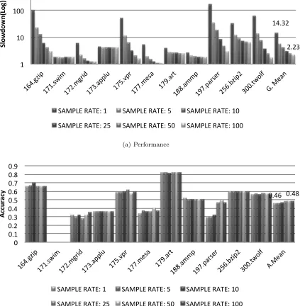
Figure 4.2 shows the performance and accuracy plots for a hash-table profiler which uses the Knuth hash function [18]. This is a function level hash table profiler, where each function has a stack allocated hash table on each invocation. The table contains 50,000 entries. The figure shows the variation in performance and accuracy when the sample rate is increased from 1 (no sampling) to 100. The performance improves by 3x - from 6x to 2x - while the accuracy doesn’t change. There are two observations that can be made from these numbers.

• The accuracy of the profiler does not appear to degrade with increased sampling. In fact, sampling appears to have little effect on accuracy.

• In the sampling technique adopted here, the performance improvement from higher sam-pling rates appears to taper off around sample rate of 100.

This is similar in design to the profiler proposed by Chen et al. in [9]. The profiler has been tailored, as described in Section 4.1.2.

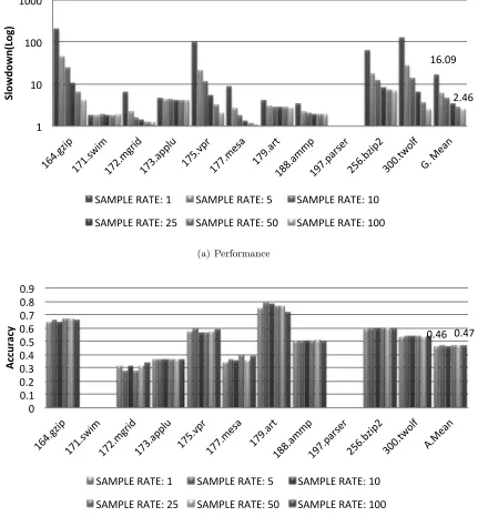
Figure 4.3 shows the performance and accuracy variation through sampling, for hash tables of size 105_{. The larger size of the table leads to higher operations costs, but the pattern seen} in the previous figure is reinforced here. The accuracy improves negligibly while performance improves significantly.

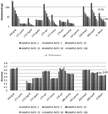
Figure 4.4 shows the performance and accuracy variation through sampling, for a hash table of size 2∗105_{. The performance and accuracy for parser are zeroes because it runs out} of memory when using a hash table of this size. The fact that sampling doesn’t improve or deteriorate accuracy leads to two important observations.

• The sampling technique shown here does in fact retain coverage, and provide a represen-tative picture even at higher sampling rates.

• The loss of accuracy in the hash tables occurs uniformly accross function calls, rather than on a small subset of the calling contexts for a given function.

(40)

14.32& 2.23& 1& 10& 100& 1000& 164.g zip& 171.swi m& 172. mgri d& 173.ap plu& 175. vpr& 177.m esa& 179.ar t& 188.am mp& 197.p arser& 256.b zip2& 300.tw olf& G.&Me an& Slowdown(Log)+

SAMPLE&RATE:&1& SAMPLE&RATE:&5& SAMPLE&RATE:&10& SAMPLE&RATE:&25& SAMPLE&RATE:&50& SAMPLE&RATE:&100&

(a) Performance 0.46% 0.48% 0% 0.1% 0.2% 0.3% 0.4% 0.5% 0.6% 0.7% 0.8% 0.9% 164.g zip% 171.swi m% 172.mgri d% 173.ap plu% 175.vp r% 177.m esa% 179.ar t% 188.am mp% 197.p arser% 256.b zip2% 300.tw olf% A.Me an% Ac cu ra cy '

SAMPLE%RATE:%1% SAMPLE%RATE:%5% SAMPLE%RATE:%10% SAMPLE%RATE:%25% SAMPLE%RATE:%50% SAMPLE%RATE:%100%

(b) Accuracy

Figure 4.2: Impact of sampling on Streamlined Hash Tables with 50000 entries

(41)

16.09& 2.46& 1& 10& 100& 1000& 164.g zip& 171.swi m& 172. mgri d& 173.ap plu& 175. vpr& 177.m esa& 179.ar t& 188.am mp& 197.p arser& 256.b zip2& 300.tw olf& G.&Me an& Slowdown(Log)+

SAMPLE&RATE:&1& SAMPLE&RATE:&5& SAMPLE&RATE:&10& SAMPLE&RATE:&25& SAMPLE&RATE:&50& SAMPLE&RATE:&100&

(a) Performance 0.46% 0.47% 0% 0.1% 0.2% 0.3% 0.4%0.5% 0.6%0.7% 0.8% 0.9% 164.g zip% 171.swi m% 172. mgri d% 173.ap plu% 175. vpr% 177.m esa% 179.ar t% 188.am mp% 197.p arser% 256.b zip2% 300.tw olf% A.Me an% Ac cu ra cy '

SAMPLE%RATE:%1% SAMPLE%RATE:%5% SAMPLE%RATE:%10%

(b) Accuracy

(42)

23.92% 2.89% 1% 10% 100% 1000% 164.g zip% 171. swim% 172.mgri d% 173.ap plu% 175.vp r% 177.m esa% 179.ar t% 188.am mp% 197.p arser% 256.b zip2% 300.tw olf% G.%Me an% Slowdown(Log)+

SAMPLE%RATE:%1% SAMPLE%RATE:%5% SAMPLE%RATE:%10% SAMPLE%RATE:%25% SAMPLE%RATE:%50% SAMPLE%RATE:%100%

(a) Performance 0.43% 0.45% 0% 0.1% 0.2% 0.3% 0.4% 0.5% 0.6% 0.7% 0.8% 164.g zip% 171.swi m% 172.mgri d% 173.ap plu% 175.vp r% 177.m esa% 179.ar t% 188.am mp% 197.p arser% 256.b zip2% 300.tw olf% A.Me an% Ac cu ra cy '

(b) Accuracy

(43)

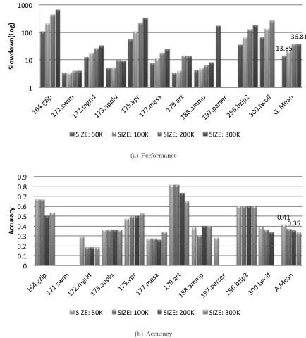
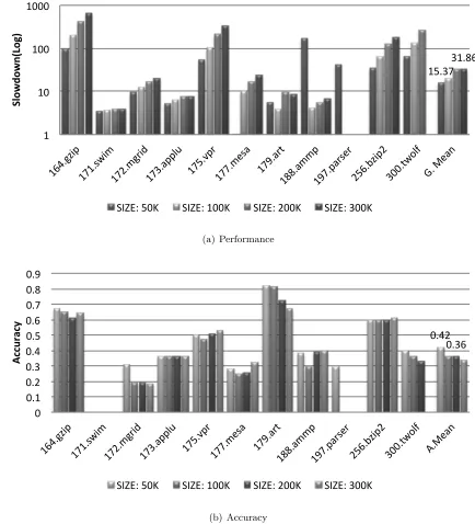
behavior ensures that this design is atleast as accurate as the streamlined design, in every case. Figures 4.6 and 4.5 show the results when using 10 and 20 tags per entry respectively. The bars represent the total memory used by the hash table (including tags). Therefore, the

13.85& 36.81& 1& 10& 100& 1000& 164.g zip& 171.swi m& 172. mgri d& 173.ap plu& 175.vp r& 177.m esa& 179.ar t& 188.am mp& 197.p arser& 256.b zip2& 300.tw olf& G.&Me an& Slowdown(Log)+

SIZE:&50K& SIZE:&100K& SIZE:&200K& SIZE:&300K&

(a) Performance 0.41% 0.35% 0% 0.1% 0.2% 0.3% 0.4% 0.5% 0.6% 0.7% 0.8% 0.9% 164.g zip% 171. swim% 172.mgri d% 173.ap plu% 175. vpr% 177.m esa% 179.ar t% 188.am mp% 197.p arser% 256.b zip2% 300.tw olf% A.Me an% Ac cu ra cy '

SIZE:%50K% SIZE:%100K% SIZE:%200K% SIZE:%300K%

(b) Accuracy

(44)

number of entries for the hash table can be calculated from the Sizeand Num Tags Per Entry as follows.

N umEntries=Size/N umT agsP erEntry

15.37&31.86& 1& 10& 100& 1000& 164.g zip& 171.swi m& 172. mgri d& 173.ap plu& 175. vpr& 177.m esa& 179.ar t& 188.am mp& 197.p arser& 256.b zip2& 300.tw olf& G.&Me an& Slowdown(Log)+

SIZE:&50K& SIZE:&100K& SIZE:&200K& SIZE:&300K&

(a) Performance 0.42% 0.36% 0% 0.1% 0.2% 0.3% 0.4% 0.5% 0.6% 0.7% 0.8% 0.9% 164.g zip% 171.swi m% 172. mgri d% 173.ap plu% 175. vpr% 177.m esa% 179.ar t% 188.am mp% 197.p arser% 256.b zip2% 300.tw olf% A.Me an% Ac cu ra cy '

SIZE:%50K% SIZE:%100K% SIZE:%200K% SIZE:%300K%

(b) Accuracy

(45)

In both the runs, 197.parser runs out of memory at 100K run itself, hence the results show zeroes for this benchmark. 300.twolf runs of memory in the 300K configuration (300,000 entries in the hash table). These results show that the performance of the hash table profiler degrades by about 1.5x at the top end (300K), while the accuracy improves from 0.46 to 0.35. The degradation in performance can be linked to the cost of inserting and checking the tags. These operations necessarily introduce a loop over the number of tags in both the insertion and membership operation.

4.3 Drawbacks

The design of hash table profiler is simple to understand, and requires simple instrumentation in the pre-profile run phase. However, the profiler has quite a few drawbacks which make it un-suitable for profiling code with complex memory access patterns, and large memory footprints.

4.3.1 Original Design

In the original design of the profiler, the memory costs increases dramatically as the number of instructions executed increases. The operations costs increase as well, since neither the hash table, nor the extendable lists provide high locality in caches. Since a virtually unlimited size structure is not feasible, in terms of memory and operations costs, most implementations restrict the amount of memory used through a fixed size table. This affects accuracy in unpredictable ways, and due to the lack of any other safety hooks in the design, this deterioration cannot be controlled. Since dependence chains are the sole source of data dependence information in this system, inaccuracy in their calculation decreases the usefulness of this data to optimizations.

Even assuming the correct calculation of dependence chains, the design only records the or-der of accesses to a given memory location. Performing relevant queries like those in Speculative Code Motion is very tough or impossible in this design. For example, given a loop, checking a load against other stores within the loop requires precise answers from the profile. In this case, that is complicated by the presence of loads and instructions from other functions which may be accessing the same memory location. This situation is made worse if the dependence chains are not calculated accurately.

(46)

since unlimited size tables are infeasible. This leads to inaccuracies which are unpredictable, as they are a product of the memory accesses and conflicts caused due to hash function.

This design improves on the original design by introducing static analyses to enable precise profiling of queries. It differs from the streamlined design, in that it uses tags to store prior addresses, rather than a single bit. This improvement allows this design to outperform the prior designs in accuracy, while suffering from performance losses due to increased operations costs. These designs show that it is tough to design a profiler than can quickly and accurately profile a large program. The root of the problem with the design of these profilers is the degree of freedom that they provide to each instruction. It is assumed that each instruction can access any given memory location, at runtime. This assumption needs to be made since there is no static analyses to provide more precise information. Arising out of this assumption, a central structure is the only way to support data dependence collection. To make lookups quick, the address of the instruction is used to index into the structure. This leads to a host of problems that were described above.

(47)

Chapter 5

Set-based Profiling using Software

Signatures

5.1 Main Idea

There are several motivating factors behind the set-based approach. First, tracking related dependences as a single set may be cheaper in terms of resources and operations performed on them. Second, by explicitly grouping related dependences together, it may be possible to improve the accuracy of profiling. Sharing resources across related dependences, which are likely to share same behavior, leads to better allocation of resources to sets, hence improving accuracy. Finally, aggressive transformations by speculative optimizations require dependence infor-mation beyond their immediate predecessors in the dependence graph. Sets allow tracking of relationships along multiple paths starting from or leading up to the candidate instruction(s).

Our set-based profiler draws inspiration from the way code optimizers work. Often, an optimizer wants to prove the absence of a dependence between one reference and a set of other references (e.g. moving a load above some stores). For convenience, let us call the instruction that is a candidate for optimization the protagonist and the other references that must be checked antagonists. If any of the antagonists inhibit optimization, then it is not possible. Hence, tracking them jointly may be sufficient since their joint answer is all that matters.

(48)

the same set since they must be disambiguated. But, we can clump protagonists with other protagonists and antagonists with other antagonists arbitrarily.

5.2 Set-Based Profiler Design

Figure 5.2 shows the key stages of our profiler. The profiler takes as input a set of queries from an analysis or optimization. These queries are interpreted as Query Sets (QSets). Each QSet consists of two groups of instructions, namely, the LHS and the RHS, and a region over which the two groups should be compared. In this work, we always consider the region to be the parent function body.

The QSets are analyzed and used to build an Interference Graph (IG) in the Interference

Graph Generation stage. Each node in the interference graph represents a set of expressions

derived from a load or store in a QSet. Edges (a.k.a interference edges) between nodes indicate that a disambiguation must be performed between the two sets; hence, they cannot be allocated to the same Profile Set (PSet). Such a lowering from QSet to IG is useful because relationships are often repeated in several QSets since individual instructions (e.g. for SCM, a store) often

st A

st B

ld X st C

ld Y

SCM Queries {ld X} ∩ {st A, st B} {ld Y} ∩ {st B, st C}

QSets qSet: LHS, RHS, Loc

1: {X}, {A, B}, {ld X} 2. {Y}, {B, C}, {ld Y}

Figure 5.1: Example showing queries and QSets.

(49)

Analysis (Speculative

Code Motion)

Interference Graph Generation

Set Allocation

Instrumen -tation LLVM

Bytecode

Queries Instrumented

LLVM Bytecode Set-based Profiler

Figure 5.2: Stages in Set-based Profiler

impact the potential to optimize other instructions (e.g. for SCM, multiple di↵erent loads). The IG is analyzed and grouped into Profile Sets (PSets) duringPSet Allocation. An expres-sion contained in a given PSet will be inserted into that set at runtime. Any interference edge in the graph indicates a membership or intersection operation that must be scheduled at runtime. Finally, the IG and PSets are input toInstrumentation which generates the instrumentation for profiling in the LLVM bitcode.

Throughout this section, we will use the example shown in Figure 5.1 to explain the process of instrumentation using sets. Figure 5.1 shows a set of example queries from SCM, which are interpreted by the profiler in terms of QSets. In this case, there are two queries. Loads X and Y are to be compared against stores A and B, and stores B and C, respectively. These queries are interpreted as two QSets, with the LHS and RHS representing the corresponding values to the compared, and the Loc specifying where the comparison operation needs to be scheduled. Given these QSets, the profiler analyses and instruments over three stages, namely, Interference Graph Generation, Set Allocation and Instrumentation. We will describe these three stages using the given example next.

5.2.1 Interference Graph Generation

Interference Graph Generation (IGG) is the stage where QSets are changed into an interference graph based representation. Interference graphs (IGs) have been used extensively as the basis for graph coloring for register allocation. We use them for a similar purpose here. They will help use map QSets into PSets. Each node in the interference graph represents a set of addresses. Edges (a.k.a interference edges) between nodes indicate that a disambiguation must be performed between the two sets; hence, they cannot be allocated to the same PSet. We have discovered two di↵erent approaches for IGG,Basic SetsandRoot Sets.

35

Figure 5.2: Stages in Set-based Profiler

impact the potential to optimize other instructions (e.g. for SCM, multiple different loads). The IG is analyzed and grouped into Profile Sets (PSets) duringPSet Allocation. An expres-sion contained in a given PSet will be inserted into that set at runtime. Any interference edge in the graph indicates a membership or intersection operation that must be scheduled at runtime. Finally, the IG and PSets are input to Instrumentation which generates the instrumentation for profiling in the LLVM bitcode.

Throughout this section, we will use the example shown in Figure 5.1 to explain the process of instrumentation using sets. Figure 5.1 shows a set of example queries from SCM, which are interpreted by the profiler in terms of QSets. In this case, there are two queries. Loads X and Y are to be compared against stores A and B, and stores B and C, respectively. These queries are interpreted as two QSets, with the LHS and RHS representing the corresponding values to the compared, and the Loc specifying where the comparison operation needs to be scheduled. Given these QSets, the profiler analyses and instruments over three stages, namely, Interference Graph Generation, Set Allocation and Instrumentation. We will describe these three stages using the given example next.

5.2.1 Interference Graph Generation

(50)

Algorithm 5:Generating interference graph for basic set allocation

Input: S: Set of Queries

Result: interf degree: Interference Graph for Queries

Result: interf: Interferences for each instruction

1 whilenot S.empty()do

2 q = S.pop();

3 foreachle∈ q.LHSdo

4 foreachre∈q.RHS do

5 insert re in interf[le];

6 insert le in interf[re];

7 insert re in interf degree[interf[re].size()];

8 end

9 insert le in interf degree[interf[le].size()];

10 end

11 end

Basic Sets

This scheme is a simple set allocation scheme which directly maps the QSets relations to the IG. Given a set of queries S, the algorithm creates a unique IG node for each SSA-name, global memory location, or stack location in the program that is present in a QSet. Then, interference edges are created between the nodes of the RHS and LHS of each QSet. This algorithm splits QSets into many different IG nodes. This creates an IG with a large number of nodes and at least one interference edge per node. The hope is that Set Allocation can merge the large number of QSets into a small number of PSets.

There are many reasons to do it this way. First, since a given memory reference is usually involved in multiple QSets, it ensures a low insertion cost since the address is only placed in one PSet globally rather than a PSet for each QSet. Second, it allows Set Allocation to keep the number PSets low (Nalloc is kept low) because it can group nodes together that have no adjoining interference edge.

The algorithm is shown in the Algorithm 5. In the algorithm, the interference degree (interf -degree) is used to track the number of interferences for each instruction. It is important to note here that each interference edge counts as a degree, even if the edge occurs multiple times in various QSets.

(51)

X

A

B

C

Y X

A

B

C

Y

Interference Edge from LHS to RHS Interference Edge between RHS members

Interference Graph for Root Sets (b)