Adaptive intelligence applied to numerical optimisation

!∀ # ∃∀%&∋(∋&

)∗)) &+∀,−)∗.∗∋(∗)(∋/∗,

01 2!33 3//.3

Adaptive intelligence applied to numerical

optimisation

Kalin Penev1 and Anton Ruzhekov2

1

Southampton Solent University, UK, [email protected] 2

Technical University of Sofia, Bulgaria, [email protected]

Abstract. The article presents modification strategies theoretical comparison and experimental results achieved by adaptive heuristics applied to numerical optimisation of several non-constraint test functions. The aims of the study are to identify and compare how adaptive search heuristics behave within heterogeneous search space without retuning of the search parameters. The achieved results are summarised and analysed, which could be used for comparison to other methods and further investigation.

Keywords: Free Search, optimisation, adaptive search heuristics, Genetic Algorithm, Particle Swarm Optimisation, Differential Evolution

1 Introduction

A previous study [10] compares Free Search (FS) [11] Particle Swarm Optimisation (PSO) [4], and Differential Evolution (DE) [14] on several heterogeneous numerical problems. This article presents another investigation, which compares modification strategies of real-value coded Genetic Algorithm BLX-α (GA BLX-α) [6], PSO [4],

DE [14] and FS [11]. In order to assess their ability for adaptation these algorithms are applied without changes of their parameters to several test problems. The aim is to compare how these algorithms behave within heterogeneous search space without retuning of the search parameters.

2

Genetic Algorithm

population of points, not from a single point; (3) GAs use payoff (objective function) information, not derivates or other auxiliary knowledge; (4) GAs use probabilistic transition rules, not deterministic rules [7]. A GAs major event is modification. It involves selection of parents, recombination between them, mutation and evaluation. For this study a Blend crossover modification strategy called BLX-α [6] is selected. For BLX-α modification strategy, the offspring is a random location within the area determined by selected parents and extended with a blend interval α. The

mathematical description of BLX-α modification strategy is presented at equation (1):

Xoffspring = Xp1 – α+ (Xp2 – Xp1 + 2α)*random(0,1). (1)

where Xp2 and Xp1 are selected parents, Xp2 > Xp1, α is a blend around the selected

parents, random(0,1) generates a random value between 0 and 1.

An extension of the space, between selected parents, increases the chances of the algorithm to reach an appropriate solution if it is near to the area determined by the parents. Variation of the blend α can be used for tuning of the search process convergence and divergence. Therefore, the concept for extension of the space for modification by a blend α is considered as valuable for improvement of the

performance of the search process. For the purposes of the investigation the GA

BLX-α is modified and implemented with a variable blend α. A low level of blend

α, benefits convergence to the optimal solution and improves effectiveness of the

search process by decreasing the number of generations necessary to attain the optimum. However, it takes a risk of being trapped in local sub-optima. A high level of blend α benefits diversification of the population and decreases the probability for

trapping in non-optimal areas, which improves the algorithm robustness. The optimisation process trapping, in a non-optimal area, cannot be resolved by variation of the blend value, due to a lack of knowledge how to tune the blend, abstracted from the current population. This problem can be a subject of further research. In summary real value GA BLX-α implicitly determines search space, as promising, with non-zero probability for generation of an offspring, and non-promising, with non-zero probability for generation of an offspring. For uni-modal problems with one optimal solution this determinism is excellent and leads to quick convergence to the appropriate solution.

However, for multi-modal problems with many, local, sub-optimal solutions this determination restricts the chances of the search process to reach an appropriate solution if it is outside of the area considered as promising from the current population. It often leads to trapping in a non-optimal solution.

3

Particle Swarm Optimisation

Xi = (xi1, xi2, ... xid). (2)

where i ∈ (1, n), n is population size (number of individuals), d is number of dimensions of the search space. Each particle maintains a memory of its previous best position:

Pi = (pi1,. pi2, ..., pid). (3)

The Particle Swarm Optimisation consists a concept for particle velocity. The velocity along each dimension is represented as:

Vi = (vi1,. vi2, ..., vid). (4)

At each iteration, the best fitness vector is memorised and denoted as g.

) (

1 i n

i P

Max g

=

= . (5)

The particles’ best achievement is denoted as vector Pi. The best achievement for

all population is denoted as vector g. The current position of the particle Xi, the best

particles’ achievement Pi and the best achievement for all population g are used for

generation of the velocity vector v for each particle (equation 6). That velocity v is then used to compute a new position for the particle (equation 7). The portion of the adjustments to the velocity influenced by the individual's previous best position Pi is

considered as an individual cognition component. The portion influenced by the best of the population is a social component [4]. With the addition of the inertia factor, w

[13] the particles are manipulated according to the following equations:

vid = w* vid + n1*random(0,1)*(Pid - xid) + n2*random(0,1)*(gd - xid). (6)

xid = xid + vid. (7)

Where the constants n1 and n2 determine the relative influence of the social and

cognitive components, and are usually both set the same to give each component equal weight as the cognitive and social learning rate. n1 is defined as the individual

learning factor and n2 is defined as the social learning factor. One of the advantages of

PSO is that there are few parameters to adjust. One version, with slight variations, works well in a wide variety of applications.

The inertia factor influences PSO positively. Large inertia factor facilitates global exploration and searching new areas, while small inertia factor tends to facilitate local exploration and fine-tunes the current search area [5].

4

Differential Evolution

generation-by-generation, into a solution vector. DE selects for manipulation target, donor and differential vectors. Therefore the minimal number of vectors in one population has to be more than four. For modification strategies, which use four differential vectors the minimal population size is seven. The current target and the corresponding new trial vector (individual) in each generation are subject of competitions to determine the composition of the next generation. The new trail vector is generated in several steps as follows: (1) selection of a randomly chosen donor vector from the population different from the current target vector; (2) selection of other (two or four) randomly chosen vectors (so called differential vectors), different from the donor, different from the current target vector and different from each other; (3) calculation of a difference between differential vectors and scaling it by multiplication with a constant called differential factor; (4) adding the difference to the donor vector, which produces a new vector; (5) crossover between the current target vector and the new vector so that the trial vector inherits parameters from both of them. If the trial vector is better than the current target vector, then the trial vector replaces the target vector in the next generation. In all, three factors control evolution under DE: the population size; the scaling weight applied to the random differential (noted as F); and the constant that mediates the number of parameters in the crossover operation. They describe DE as a heuristic approach for optimising non-linear and non-differentiable functions within continuous space [14]. Let us denote the target vector - Xk, the differential vectors - Xi

and Xj, and the differential factor (weight) - F. Every pair of vectors (Xi, Xj) in the

primary array defines a differential vector Xi - Xj.

When these two vectors are chosen randomly, their weighted difference is used to perturb another vector in the primary array, Xk':

Xk' = Xk + F(Xi - Xj). (8)

F scales the difference achieved from Xi -Xj. An effective variation of this scheme

involves keeping track of the best vector noted as X*. This can be combined with Xk

and then perturbed, producing:

Xk' = Xk + F(X* - Xk) + F(Xi - Xj). (9)

Storn proposes several modification strategies for calculation of a new individual as follows:

(1) Xk' = Xk + F(Xi - Xj). (10)

(2) Xk' = X* + F(Xi - Xj). (11)

(3) Xk' = Xk + F(X* - Xk) + F(Xi - Xj). (12)

(4) Xk' = X* + F(Xi - Xj + Xn - Xm). (23)

(5) Xk' = Xk + F(X* - Xk + Xn - Xm). (14)

where Xk is a donor vector, Xk' is mutated donor, X* is the best vector for current

population, Xi, Xj, Xn and Xm are differential vectors, F is differential factor. These

suggests that they are very similar. However, these strategies are grounded on different concepts therefore the algorithms behaviour and their results are different.

From another point of view mutation in DE is, in fact, a calculation of the sum between the donor vector and the differential of two other or four other vectors [14]. Comparison of this operation with the BLX-α real-coded crossover [6] can identify similarity between them. In the next step each primary array vector Xk is targeted for

recombination with Xk' to produce a trial vector Xt. Thus the trial vector is the child of

two parents, a noisy random vector and the primary array vector against which it must compete. Once a new trial solution has been generated, selection determines which among them will survive into the next generation. Each child Xt is pitted against its

parent Xk in the primary array. Only the fitter of the two is then allowed to advance

into the next generation.

5 Free

Search

Free Search is real value adaptive heuristic method inspired by animals behaviour in nature. The search process is organised in exploration walks, which differs from classical iterations [11]. FS modification strategy is described as follow: Xmini and

Xmaxi denote the search space borders, m is a population size, j = 1,..,m, k = 1,..,m, n

is a number of dimensions, i = 1,..,n. T is step limit per walk. t is current step. Rji is a

variable neighbouring space Rji∈ [Rmin, Rmax]. The algorithm requires definition of

search space borders [Xmini , Xmaxi ], population size m, limit for number of

explorations G, limit for number of steps per exploration T, minimal and maximal values for the neighbour space [Rmin, Rmax]. The maximal neighbour space guarantee coverage of the whole search space from one animal. The minimal neighbour space guarantee desired granularity of the coverage from one animal. Rmin

and Rmax are absolute values. An appropriate definition of these values supports successful performance across variety of problems without additional external adjustments [11]. A determination of the neighbour space to concrete value for particular problem can lead to slightly better performance on this problem but aggravates the performance on other problems, which is in line with the existing general assessment of the performance of the optimisation algorithms [15].

The exploration walk in FS generates coordinates of a new location xtji as:

xtji= x0ji - Δxtji + 2*Δxtji*randomtji(0,1). (15)

The modification strategy is:

Δxtji = Rji * ( Xmaxi – Xmini ) * randomtji(0,1). (16)

Where i = l for uni-dimensional step, i = 1,..,n for multi-dimensional step. T is step limit per walk. t is current step, t = 1,..,T. Rji indicates a neighbour space size for

animal j within dimension i. randomtji(0,1) randomises the steps within defined

6 Test

problems

For all experiments the aim is to find the maximum therefore the test functions are transformed in relevant manner. All test problems are in 2 dimensional variant. Step test function - This test function is proposed by De Jung [3]. It introduces plateaus to the topology. Maximal are all locations, which belong to the plateau x_i∈

[2.0, 2.5) and the maximum for 2 dimensions is f max =4. Maximise:

⎣ ⎦

∑

( , where xi∈ [-2.5, 2.5]. (17)

Step sphere test function - It introduces also plateaus to the topology, and also excludes a local correlation of the space. [2] Maximal are all locations, which belong to the plateau x_i∈ [-0.5, 0.5). The maximum is f max =10. Maximise:

⎣

∑

(

⎦

(18)

Michalewics test function - The Michalewics test function is described in the domain of Kyoto University [8]

m i i i ix x x x f 2 2 1 2 2

1, ) sin( )(sin( / ))

(

∑

=

= . (19)

whre i=2, m=10, xi∈ [0.0, 3.0]. For two dimension maximum is f(x1, x2) = 1.8013

Five hills test function - The Five hills test function is designed for this investigation based on the equation 20 below, where x_i∈ [-10.0, 10.0] and i=2.

f(x1, x2) = 9.4/(1+0.05*((-x1)2+ (-x2)2)) + 9.5/(1+1.7*((7-x1)2+ (7-x2)2))+

9.6/(1+1.7*((7+x1)2+ (7+x2)2)) + 9.7/(1+1.7*((7-x1)2+ (7+x2)2))+

10.0/(1+1.7*((7+x1)2+ (7-x2)2)).

(20)

7 Experimental

results

GA, PSO, DE and FS are applied to the above-mentioned functions as follows – Each algorithm is evaluated four times per test function – (1) start from stochastic initial population with limit 100 iterations, (2) start from stochastic initial population with limit 2000 iterations, (3) start from one initial location with limit 100 iterations, (4) start from one initial location with limit 2000 iterations. The single initial location is defined as: x0 = xmin + 0.9(xmax - xmin). Each evaluation is 320 experiments. Population

size is 10 (ten) individuals for all algorithms for all experiments. For GA the bled α

Table 1. Experimental results

Heading level F1 F2 F3 F4 Overall

FS R*-100 320 320 224 67 931

FS R-2000 320 320 320 218 1174

FS OL*-100 320 320 227 74 941

FS OL-2000 320 320 320 214 1178

DE R-100 320 320 318 53 1011

DE R-2000 320 320 319 59 1018

DE OL-100 - - -

DE OL-2000 - - -

PSO R-100 320 320 130 10 780

PSO R-2000 320 320 169 54 863

PSO OL-100 - - -

PSO OL-2000 - - -

GA R-100 226 244 0 0 470

GA R-2000 320 320 8 6 654

GA OL-100 270 314 0 0 584

GA OL-2000 320 320 16 2 658

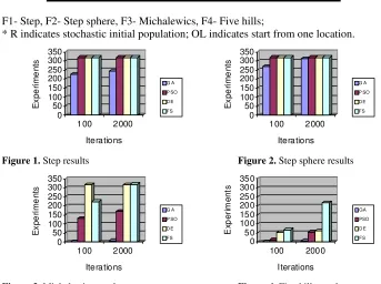
F1- Step, F2- Step sphere, F3- Michalewics, F4- Five hills;

* R indicates stochastic initial population; OL indicates start from one location.

0 50 100 150 200 250 300 350 Ex p e ri m e n ts 100 2000 Iterations G A P SO D E FS 0 50 100 150 200 250 300 350 E x pe ri m e nts 100 2000 Iterations G A P SO D E FS

Figure 1.Step results Figure 2. Step sphere results

0 50 100 150 200 250 300 350 Ex p e ri m e n ts 100 2000 Iterations GA PSO D E FS 0 50 100 150 200 250 300 350 E x pe ri m e nts 100 2000 Iterations G A P SO D E FS

Figure 3. Michalewics results Figure 4. Five hills results

The results presented on Table and Figures suggest that PSO, FS and DE can solve these four tests within 100 iterations, and within 2000 iterations almost any run leads to successful result. DE and PSO due to their modification strategise cannot start form one location. GA begins effective search after the first mutation and has less success.

demonstrates the highest convergence speed. However on global optimization such as Five hills test the experimental results show that the high convergence speed aggravates adaptation and leads to trapping in local sub optima.

8 Conclusion

The article compares modification strategies of GA BLX-α, PSO, DE and FS and their ability to adapt to four non-constrained tests. Explored algorithms show good capabilities for adaptation to different problems without supervisor’s control and without additional adjustment to the concrete problem. This study demonstrates that FS has higher overall performance on explored test. It confirms also Free Search can advance a wide range of disciplines in the efforts to cope with complex problems. Further investigations can focus on replacement strategies comparison and evaluation. A pragmatic area for further research is application to communication tasks such as optimisation of MIMO (multiple inputs multiple outputs) communication systems.

References

1. Angeline P., 1998, Evolutionary Optimisation versus Particle Swarm Optimisation: Philosophy and Performance Difference, The 7-th Annual Conference EP, San Diego, USA. 2. Bäck T., and Schwefel H.-P., 1993, An overview of evolutionary algorithms for parameter

optimisation, Evolutionary Computation, 1:1, pages (1-23).

3. De Jong K., 1975, An Analysis of the Behaviour of a Class of Genetic Adaptive Systems, PhD Thesis, University of Michigan.

4. Eberhart R. and J. Kennedy, 1995, Particle Swarm Optimisation, Proceedings of the 1995 IEEE International Conference on Neural Networks., vol. 4, 1942-1948.

5. Eberhart R., and Shi Y., 1998, Comparison between Genetic Algorithms and Particle Swarm Optimisation, The 7-th Annual Conference on Evolutionary Programming, San Diego, USA. 6. Eshelman L. J., and Schaffer J. D., 1993, Real-coded genetic algorithms and interval-schemata, Foundations of GA 2, Morgan Kaufman Publishers, San Mateo, pages (187-202). 7. Goldberg D.E., 1989, Genetic Algorithms in Search, Optimisation, and Machine Learning,

Addison Wesley Longman Inc. ISBN 0-201-15767-5.

8. Hedar A.R., 2010, Global Optimisation, Kyoto University, http://www-optima.amp.i.kyoto-u.ac.jp/member/student/hedar/Hedar_files/TestGO_files/Page2376.htm, last visited 02.06.10 9. Holland J., 1975, Adaptation In Natural and Artificial Systems, Uni. of Michigan Press. 10. Penev K., and Littlefair G., 2005, Free Search – A Comparative Analysis, Information

Sciences Journal, Elsevier, Volume 172, Issues 1-2, pp 173-193

11. Penev K., 2008, Free Search of Real Value or How to Make Computers Think, Alexander Gegov (Editor), St. Qu publisher, April 2008, ISBN 978-0955894800, UK.

12. Price K., and R. Storn, 1997, "Differential Evolution", Dr, Dobb's Journal 22 (4), 18-24. 13. Shi Y. and Eberhart R. C., 1998, Parameter Selection in Particle Swarm Optimisation,

Evolutionary Programming VII (1998), LNCS 1447, pages (591-600), Springer.

14. Storn R. and Price K., 1995, Differential Evolution – A simple and efficient adaptive scheme for global optimisation over continuous spaces, TR-95-012, International Computer Science Institute, 1947 Center Street, Berkeley, CA 94704-1198, Suite 600.