Network-meta analysis made easy: detection of inconsistency using factorial analysis-of-variance models

R E S E A R C H A R T I C L E

Open Access

Network-meta analysis made easy: detection of

inconsistency using factorial analysis-of-variance

models

Hans-Peter Piepho

Abstract

Background:Network meta-analysis can be used to combine results from several randomized trials involving more than two treatments. Potential inconsistency among different types of trial (designs) differing in the set of treatments tested is a major challenge, and application of procedures for detecting and locating inconsistency in trial networks is a key step in the conduct of such analyses.

Methods:Network meta-analysis can be very conveniently performed using factorial analysis-of-variance methods. Inconsistency can be scrutinized by inspecting the design × treatment interaction. This approach is in many ways simpler to implement than the more common approach of using treatment-versus-control contrasts.

Results:We show that standard regression diagnostics available in common linear mixed model packages can be used to detect and locate inconsistency in trial networks. Moreover, a suitable definition of factors and effects allows devising significance tests for inconsistency.

Conclusion:Factorial analysis of variance provides a convenient framework for conducting network meta-analysis, including diagnostic checks for inconsistency.

Keywords:Analysis of variance, Baseline contrast, Heterogeneity, Inconsistency, Linear mixed model, Network meta-analysis, Pairwise treatment contrast, PRESS residual, Studentized residual

Background

Results from several randomized trials can be combined by meta-analysis methods. In the simplest case, all trials comprise the same set of treatments, typically only two, i.e., a new treatment and a control or baseline treatment. When trials differ in design, i.e., in the sets of treatments tested, joint analysis may be done by what has come to be called network meta-analysis (NMA). Such analyses combine different sources of pairwise treatment compa-risons across trials, i.e., direct compacompa-risons from trials that jointly test both treatments of interest and indirect comparisons from trials that only test one of the two treatments, but are connected through other treat-ments via the trial network. A key assumption of many methods for NMA is consistency of treatment effect esti-mates across designs, defined by the set of treatments

tested. In particular, consistency implies agreement be-tween direct and indirect evidence on a treatment con-trast. Several methods have been proposed for detecting inconsistency in trial networks [1-4].

Most methods for analysis of NMA operate on pair-wise contrasts of treatments with a baseline treatment or control, henceforth denoted as baseline contrasts. Some methods for detecting inconsistency in meta-analysis networks based on baseline contrasts are relatively complex on account of the fact that baseline treatments may vary among trials and sources of inconsistency have to be traced through loops of the network [3-5]. It has been shown by Piepho et al. [6] that NMA can be greatly simpli-fied by modelling treatment means rather than treatment contrasts using factorial analysis-of-variance (ANOVA) models, and that such analyses can produce identical or essentially the same results as analyses using baseline contrasts. The present paper will therefore focus on the ANOVA approach and illustrate its versatility. Specifically,

Correspondence:[email protected]

Bioinformatics Unit, Institute of Crop Science, University of Hohenheim, Fruwirthstrasse 23, 70599 Stuttgart, Germany

we will explore ways to detect inconsistency using standard procedures for linear models available in most statistical packages. The methods will be illustrated using the dia-betes example published by Senn et al. [7]. This example has also been used by Krahn et al. [1] to illustrate their pro-posed methods for detection of inconsistency using a base-line contrast parameterization, so our results can be compared directly to that paper in order to appreciate the degree of agreement between both model formulations and the resulting tests and diagnostic checks for inconsist-ency. The presentation assumes that the reader has access to a mixed model package using restricted maximum likeli-hood (REML) to estimate variance components and is fa-miliar with the essentials of the underlying theory [8]. Program code in SAS for all analyses presented is given in Additional file 1.

Methods

In this section, we describe the basic models we are using. In the Results section, minor extensions and asso-ciated statistics derived from the various models, such as influence diagnostics, are introduced as needed.

A two-way ANOVA model for meta-analysis can be written as

ηij¼βiþγjþuij ð1aÞ

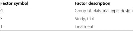
where η_ij is the expected value of the j-th treatment in the i-th trial, β_i is the main effect of the i-th trial, γ_j is the main effect of the j-th treatment, and u_ij is a trial × treatment interaction effect, which models hetero-geneity between trials. For implementation it is convenient to represent the linear model (1a) in symbolic notation that is akin to model syntax used in linear model packages. We here use a notation originally proposed by Wilkinson and Rogers [9], which has hence been used by many authors [10,11] and has also been implemented in some linear model packages. The factors used for representing the model are given in Table1.

The two-way ANOVA model (1) can be represented as [9]

ST¼SþTþS:T ð1bÞ

where × is an operator for crossing two factors or model terms, S is a factor identifying the individual trial, and T denotes the treatment factor. Effects in (1b) can be

equated with those in (1a) as follows: S ≡ βi, T ≡ γj,

and S.T ≡uij.

In NMA, trials can be classified into groups of trials according to the set of treatments tested. These categories will henceforth be denoted as designs (Table 1). Procedures for detecting inconsistency can be easily implemented by expanding the ANOVA model (1) to reflect the nesting of trials within designs. The extended model is

ηhij¼αhþβhiþγjþvhjþuhij ð2aÞ

whereαhis a main effect for theh-th design,βhiis an

ef-fect for the i-th trial nested within theh-th design,γjis

the main effect of thej-th treatment,vhjis an interaction

effect for theh-th design and thej-th treatment, anduhij

is an interaction effect for the i-th trial (nested within the h-th design) and the j-th treatment. The interaction effect vhj represents inconsistency, whereas uhij

repre-sents heterogeneity as in model (1) [6,12]. Using the fac-tor G to represent the design (Table 1), the symbolic version of the extended model (2a) is

G=S

ð Þ T¼GþG:SþTþG:TþG:S:T ð2bÞ

where / is a nesting operator [9]. Note that the nesting relation G/S in (2b) is resolved as G/S = G + G.S. This structure is then fully crossed with T, as indicated by the crossing operator × on the left-hand side of eq. (2b). Ef-fects in (2a) and (2b) can be equated as follows: G≡αh,

G.S≡βhi, T≡γj, G.T≡vhj, and G.S.T≡uhij.

Linear predictors (1) and (2) can be used either in models for individual patient data or in models for treatment summaries per trial (e.g., empirical logits or treatment means) [6]. When individual patient data are modelled, then depending on the outcome variable it may be appropriate to use the linear predictor in a generalized linear (mixed) model [GL(M)M], e.g., when the response is binomial so that a logit or probit link is required. When summary measures are available, it is customary to model the response by a linear (mixed) model assuming normal-ity and accounting for possible heterogenenormal-ity in precision by weighting. In the diabetes example by Senn et al. [7], we have at our disposal mean responses per treatment and trial as well as the associated sample standard deviations and sample sizes, from which the variance of a mean can be computed. Thus, the models used for our analyses are of the form

y¼ηþe ð3Þ

where y is the observed treatment mean in a trial, ηis the linear predictor, modelled, e.g., using (1) or (2), ande is the random normal error associated with the observed mean. The errors are modelled to have zero mean and variance var(e) equal to the observed squared standard error of a mean, assumed to be a known constant when Table 1 Description of factors used for representing

factorial ANOVA models for NMA

Factor symbol Factor description

G Group of trials, trial type, design

S Study, trial

fitting (3). This analysis is easily performed using linear mixed model software with weighting facility by defining the inverse of var(e) as weight and fixing the residual variance at unity [13]. The approach is fully efficient, be-cause the variance-covariance matrix of the vector of meansyis diagonal with elements equal to var(e) [14].

Following Krahn et al. [1], we will initially consider analyses by models (1) and (2) when all effects in the linear predictor (eq. 1b or 2b) are taken as fixed. Subse-quently, we will consider analyses that model heterogen-eity [i.e., the interaction effects S.T and G.S.T in eqs. (1b) and (2b), respectively] as random, which is common practice (see, e.g., [6] and [15]). One may argue that if heterogeneity is detected, then the effect for heterogen-eity may be used as an error term for testing inconsist-ency because heterogeneity effects are nested within the effects for inconsistency. This leads to an analysis with random interaction effects S.T or G.S.T. Conversely, one may insist that heterogeneity be modelled as a fixed effect. Then if heterogeneity is detected, it may be con-cluded that there is no further basis for testing inconsist-ency because of the nested structure of effects for heterogeneity in relation to inconsistency. In this situ-ation, one may try to find subsets of trials that do not dis-play heterogeneity and analyse these subsets separately [2]. This philosophy is in agreement with that put for-ward by Nelder [16], who argued that testing main effects in a two-way fixed-effects ANOVA is justified only when the interaction is deemed to be absent and the model is reduced accordingly. Here, we will present results for both approaches (interactions for heterogeneity fixed or random) and compare the results. Our favoured ap-proach is to model heterogeneity as random when per-forming checks and tests for inconsistency as well as when comparing treatment means.

Results

The diabetes data comprise a total of 26 trials, most of which involve a glucose lowering agent added to a base-line sulfonylurea therapy. The continuous outcome vari-able is blood glucose change as measured by the marker HbA1c in patients with type two diabetes. There were fifteen different designs, including one three-armed trial and fourteen trials involving only two treatments. The network provides direct evidence for fifteen out of 45 possible pairwise contrasts. Eight of these contrasts in-volve the placebo. The ten different treatments are given in Table 2.

Fitting models (1) and (2)

We start by fitting models (1) and (2) as purely fixed ef-fects models, which is equivalent to the models used by Krahn et al. [1]. Generally, throughout the example, we adhere to the order of effects as stated in models (1) and

(2) and use sequential (incremental) fitting of terms, cor-responding to Type I hypotheses in linear model proce-dures of the SAS system, which is used for all analyses presented in this paper. There are five designs that have more than one trial and so allow testing for heterogen-eity. Thus, we first fit model (1) separately to each of these designs. The resulting Wald-type chi-squared sta-tistics for significance of the trial × treatment interaction (u_ij), along with the associated p-values, are shown in Table 3. There is significant heterogeneity for four out of five designs.

An overall test for heterogeneity is obtained by fitting model (2). The trial × treatment interaction (G.S.T) yields a chi-squared statistic of 74.45 on 11 d.f. (p< 0.0001). This chi-squared statistic for overall heterogeneity is equal to the sum of the chi-squared statistics for heterogeneity for the five designs in Table 3. When dropping the effect G.T from the model, the Wald-test for the effect G.S.T be-comes a joint test for inconsistency and heterogeneity. The chi-squared statistic for this test equals 96.98 on 18 d.f. (p< 0.0001), and it is equal to Generalized Cochran’s Q [1]. Further note that the model T + S + T.S produces the same overall Q of 96.98. At this point, we can con-clude that there is significant heterogeneity.

All chi-squared statistics presented so far are identical to those in Table 3 of Krahn et al. [1], who used a model

Table 2 Ten treatment groups of the diabetes example of Senn et al. [7]

Four-letter abbreviation of treatment Treatment

acar Acarbose

benf Benfluorex

metf Metformin

migl Miglitol

piog Pioglitazone

plac Placebo

rosi Rosiglitazone

sita Sitagliptin

SUal Sulfonylurea alone

vild Vildagliptin

Table 3 Wald-type chi-squared tests for heterogeneity (u_ij) Design Wald

statistic

Number of studies

Degrees of freedom p

-value

benf:plac 4.38 2 1 0.0363

metf:plac 42.16 3 2 <0.0001

migl:plac 6.45 3 2 0.0398

rosi:plac 21.27 6 5 0.0007

rosi:metf 0.19 2 1 0.6655

based on baseline contrasts. We also obtain their chi-squared statistic for inconsistency, when we fit G.S.T as fixed and test the effect G.T (chi-squared = 22.53, d.f. = 7,p= 0.0021). But we favor a mixed model analysis with random trial × treatment interaction (G.S.T), be-cause we consider it the major error term for testing the design × treatment interaction (G.T), which assesses in-consistency. At the same time, the trial effect needs to be modelled as fixed in order to maintain equivalence with the baseline contrast approach [6,7]. When we take the interaction effect for heterogeneity (G.S.T) as random, assuming a constant variance for this effect, the chi-squared statistic for inconsistency (G.T) drops to 2.27. The REML estimate of the variance for heterogeneity is

^ σ2

u¼0:06932. Note that this estimate corresponds to half the variance for heterogeneity with the baseline contrast approach [6,15] (usually denoted asτ2). Since the test for inconsistency now involves an estimated variance com-ponent, we use the Kenward-Roger method for approxi-mating the denominator d.f. of a Wald-type F-statistic [17]. We findF= 0.32 on 7 numerator and 11 denomin-ator d.f. and p= 0.9268. By this analysis, there is no sig-nificant inconsistency, which is in contrast to the analysis with fixed effects for G.S.T. Note that this analysis treats the residual variances of the individual trials as known constants, although they are, in fact, estimated when ana-lysing individual trials. The added uncertainty associated with these variance estimates could be accounted for by using the Kenward-Roger method in a single-stage ana-lysis modelling individual patient data [14], but differ-ences compared to the two-stage analysis employed here are expected to be small so long as the sample sizes per treatment and trial are large enough, as is usually the case.

A very simple further check for inconsistency is to fit both G.T and G.S.T as random. The best linear unbiased predictors (BLUPs) of the G.T effects give a direct indi-cation which treatment × design combinations contribute most to the inconsistency. With the diabetes example, the variance component for G.T is estimated to be zero, so the BLUPs for all G.T effects are zero, which is in agreement with the non-significant Wald-test for inconsistency.

Locating inconsistency by detachment of individual designs

Locating inconsistency in the network may be based on a detachment of an individual design from the others by a suitable model formulation that allows testing the con-tribution of that individual design to inconsistency in the network as well as the inconsistency that remains after detaching that design. Krahn et al. [1] showed how to code a detachment model for baseline contrasts. Here, we show how to implement this approach based on a straight-forward extension of the factorial model (2).

To illustrate, consider the first design in the diabetes example, which has fifteen designs, coded by a factor G. We may define a new factor D1 for the first design, which has two levels, one for the first design and an-other common level for the remaining fourteen designs (Table 4). Obviously, factors D1 and G have a hierarch-ical relationship, with G nested in D1. Thus, the inter-action effect G.T, which assesses inconsistency, may be partitioned as

D1=G

ð Þ:T¼D1:TþD1:G:T ð4Þ

Fitting both effects on the right-hand side of (4) simul-taneously, the effect D1.T captures the contribution of the first design to the overall design × treatment inter-action, i.e., to overall inconsistency, while the remainder of the interaction/inconsistency after detachment of the first design is captured by the effect D1.G.T. Using the syntax of Wilkinson and Payne [9] and observing the nesting of factors D1, G and S, the full model can be de-veloped as follows:

D1=G=S

ð ÞT¼D1þD1:GþD1:G:SþT

þD1:TþD1:G:TþD1:G:S:T ð5Þ

The same partitioning can be done, in turn, for each of the other fourteen designs. The coding for factors Dk [k∈(1,…,15)], where kindexes the designs, is shown in Table 4. Table 5 shows the results of analysis by model (5) for the eleven out of fifteen designs which contribute to the design × treatment interaction of the network. The analysis was done taking the interaction for hetero-geneity (D1.G.S.T) either as fixed or random. Note that in case of a fixed effect for heterogeneity the Wald-type chi-squared statistics for D1.T and D1.G.T in (5) (see Table 5) add up to the chi-squared statistic for overall inconsistency (G.T) in (2) (chi-squared = 22.53), but not when heterogeneity is modelled as random. When the heterogeneity effect is modelled as fixed, there are five designs with a significant contribution to the inconsist-ency (Table 5). The strongest contribution comes from the design rosi:SUal, which was also detected by Krahn et al. [1] as being the major source of inconsistency. For this design, as well as for the design metf:SUal, the test of the remainder of the inconsistency (Dk.G.T) is non-significant, suggesting that one of these designs could be removed to instate consistency. When heterogeneity is modelled as random, however, there is no indication of inconsistency for any of the designs.

model (2). In the second stage, we fit an additive two-way model of the form G + T to the design × treatment means. From this analysis, we can obtain residual and influence diagnostics [18,19] by standard procedures with most linear mixed model packages. The key idea is that observa-tions contributing substantially to inconsistency will dis-play strong G.T interaction effects, which in turn will be captured by the residuals of the additive model G + T.

Three different options are considered for handling the effect for heterogeneity (G.S.T) in the first-stage ana-lysis based on model (2): (i) taking it fixed, (ii) taking it random and (iii) dropping it. It turns out that with op-tions (ii) and (iii), the treatment means of designs 3, 4, 7, 11 and 12 are correlated, meaning that weighting by the inverse of the squared standard errors is only an approximate method (note that the designs in question

Table 4 Definition of detachment factors for testing inconsistency [Dk.T;k∈(1,…,15)]

Design (factor G)

Design no. (_k)

Factor for detachment

Level of factor for the fifteen designs

1 2 3 4 5 6 7 8 9 10 11 12 13 14 15

acar:plac 1 D1 1 0 0 0 0 0 0 0 0 0 0 0 0 0 0

acar:SUal 2 D2 0 1 0 0 0 0 0 0 0 0 0 0 0 0 0

benf:plac§ _{3 - - - - - - - - - - - - - - -}

-metf:plac 4 D4 0 0 0 1 0 0 0 0 0 0 0 0 0 0 0

metf:acar:plac 5 D5 0 0 0 0 1 0 0 0 0 0 0 0 0 0 0

metf:SUal 6 D6 0 0 0 0 0 1 0 0 0 0 0 0 0 0 0

migl:plac§ _{7 - - - - - - - - - - - - - - -}

-piog:plac 8 D8 0 0 0 0 0 0 0 1 0 0 0 0 0 0 0

piog:metf 9 D9 0 0 0 0 0 0 0 0 1 0 0 0 0 0 0

piog:rosi 10 D10 0 0 0 0 0 0 0 0 0 1 0 0 0 0 0

rosi:plac 11 D11 0 0 0 0 0 0 0 0 0 0 1 0 0 0 0

rosi:metf 12 D12 0 0 0 0 0 0 0 0 0 0 0 1 0 0 0

rosi:SUal 13 D13 0 0 0 0 0 0 0 0 0 0 0 0 1 0 0

sita:plac§ _{14 - - - - - - - - - - - - - - -}

-vild:plac§ _{15 - - - - - - - - - - - - - - -}

-Factors are defined for eleven designs in the diabetes example of Senn et al. [7] (due to the network structure, the other four designs do not contribute to the inconsistency).

§

These designs do not contribute to the overall inconsistency interaction design × treatment (G.T).

Table 5 Wald-type chi-squared tests for inconsistency using detachment factors [Dk.T;k∈(1,…,15)]

Design Design no. (k)

Number of studies

Degrees of freedom for Dk.T

Effect Dk.G.S.T fixed Effect Dk.G.S.T random

D_k.T D_k.G.T D_k.T D_k.G.T

Wald statistic

p-value Wald statistic

p-value Wald statistic

p-value§ _Wald

statistic

p-value§

acar:plac 1 1 1 0.09 0.7699 22.45 0.0010 0.02 0.8889 2.25 0.8782

acar:SUal 2 1 1 0.01 0.9091 22.52 0.0010 0.01 0.9430 2.26 0.8765

metf:plac 4 3 1 0.46 0.4976 22.07 0.0012 0.04 0.8379 2.22 0.8814

metf:acar:plac 5 1 2 0.15 0.9297 22.39 0.0004 0.07 0.9634 2.18 0.8129

metf:SUal 6 1 1 15.02 0.0001 7.52 0.2758 1.63 0.2343 0.92 0.9835

piog:plac 8 1 1 5.28 0.0215 17.25 0.0084 0.43 0.5299 1.96 0.9062

piog:metf 9 1 1 5.40 0.0201 17.13 0.0088 0.43 0.5318 1.94 0.9081

piog:rosi 10 1 1 0.05 0.8280 22.49 0.0010 0.01 0.9065 2.27 0.8751

rosi:plac 11 6 1 6.24 0.0125 16.30 0.0122 0.74 0.4112 1.87 0.9168

rosi:metf 12 2 1 0.01 0.9199 22.52 0.0010 0.01 0.9276 2.25 0.8795

rosi:SUal 13 1 1 15.76 <0.0001 6.77 0.3424 1.79 0.2146 0.66 0.9930

Tests are reported for eleven detached designs in the diabetes example of Senn et al. [7] (due to the network structure, the other four designs did not contribute to the inconsistency). The effect Dk.G.S.T was taken either as fixed or as random. Tests significant at the 5% level are boldfaced.

§

are precisely the ones represented by several trials). An exact analysis requires carrying the full variance-covariance matrix of design × treatment means forward and specifying this as the residual variance-covariance matrix of the model fitted at the second stage [14]. This is easily done in SAS using the REPEATED state-ment with the option TYPE = LIN(1). Note that option (iii) is in line with common practice when the baseline contrast formulation is used [1] and heterogeneity is

deemed absent. But heterogeneity was found to be sig-nificant for the diabetes data, so one may argue that this effect should be in the model for checking consistency. If the effect is in the model and taken as fixed (option i), effectively all trials are given the same weight, whereas when the effect is dropped (option iii), each trial is weighted according to the variances of the means, which explains the differences in results. Both analyses are not fully satisfactory because heterogeneity is not

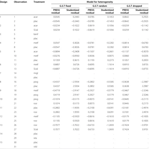
Table 6 Studentized residuals and PRESS residuals

Design Observation Treatment Model for heterogeneity

G.S.T fixed G.S.T random G.S.T dropped

PRESS residual

Studentized residual

PRESS residual

Studentized residual

PRESS residual

Studentized residual

1 1 acar 0.0545 0.2443 0.0785 0.1453 0.0642 0.2925

2 plac −0.0545 −0.2443 −0.0785 −0.1453 −0.0642 −0.2925

2 3 acar −0.0234 −0.1022 0.0619 0.1056 −0.0259 −0.1142

4 SUal 0.0234 0.1022 −0.0619 −0.1056 0.0259 0.1142

3 5 benf

6 plac . . . .

4 7 metf 0.0547 0.3026 −0.0781 −0.2282 −0.0814 −0.6783

8 plac −0.0547 −0.3026 0.0781 0.2282 0.0814 0.6783

5 9 acar −0.0894 −0.2408 −0.1507 −0.2601 −0.1137 −0.3070

10 metf −0.0276 −0.0930 0.0036 0.0075 0.0060 0.0205

11 plac 0.1359 0.3615 0.1193 0.2273 0.1057 0.2833

6 12 metf 0.6807 3.6726 0.6095 1.1614 0.6910 3.8755

13 SUal −0.6807 −3.6726 −0.6095 −1.1614 −0.6910 −3.8755

7 14 migl . . . .

15 plac . . . .

8 16 piog −0.4337 −2.5934 −0.2802 −0.5585 −0.3638 −2.2987

17 plac 0.4337 2.5934 0.2802 0.5585 0.3638 2.2987

9 18 metf −0.4719 −2.9147 −0.2927 −0.5779 −0.3467 −2.3246

19 piog 0.4719 2.9147 0.2927 0.5779 0.3467 2.3246

10 20 piog −0.1074 −0.5173 −0.0073 −0.0141 −0.0445 −0.2173

21 rosi 0.1074 0.5173 0.0073 0.0141 0.0445 0.2173

11 22 plac −0.2802 −1.9593 −0.2100 −0.6391 −0.3181 −2.4974

23 rosi 0.2802 1.9593 0.2100 0.6391 0.3181 2.4974

12 24 metf −0.1105 −0.5920 −0.0616 −0.1610 −0.0179 −0.1005

25 rosi 0.1105 0.5920 0.0616 0.1610 0.0179 0.1005

13 26 rosi −0.7077 −3.7022 −0.6733 −1.2693 −0.7424 −3.9701

27 SUal 0.7077 3.7022 0.6733 1.2693 0.7424 3.9701

14 28 plac . . . .

29 sita . . . .

15 30 plac . . . .

31 vild . . . .

appropriately taken into account. Taking heterogeneity as random (option ii) is common practice in meta-analysis [6,15], and this is also our preferred approach over option (i) for the reasons stated at the end of the Methods section.

To compute influence diagnostics in stage two, we here use the output generated by the INFLUENCE op-tion to the MODEL statement of the MIXED procedure of SAS (Version 9.4). The PRESS residuals and studen-tized residuals are shown in Table 6. The PRESS residual for the m-th observation is the raw residual when the

m-th observation has been deleted for estimating the fitted value. Large residuals indicate design × treatment combinations contributing substantially to the overall in-consistency. When in the first stage the effect for hetero-geneity in model (2) (G.S.T) is modelled as fixed, or when the effect for heterogeneity is dropped, then de-signs 6 and 13 stand out as having conspicuously large studentized residuals relative to the standard normal dis-tribution and relatively large PRESS residuals, which is in agreement with the tests in Table 5 and also with the results by Krahn et al. [1]. When heterogeneity is mod-elled as random, however, the studentized residuals of all designs are inconspicuous, which also agrees with our results in Table 5. The agreement of results based on PRESS residuals with the tests in Table 5 is expected be-cause the Dkfactor essentially invokes a deletion oper-ation that separates the effect of the k-th design from the rest, which is exactly the effect of PRESS residuals computed here (Table 6). It is noted that the residuals of two-treatment designs are equal in absolute value and of opposite sign, as expected. Observations with no resid-uals correspond to designs that do not contribute to the design × treatment interaction in the network.

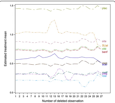
A further set of useful diagnostic statistics are the case-deletion estimates of treatment means. Figure 1 shows a case-deletion plot for all treatment means against observations that contribute to the design × treatment interaction. The analysis is based on design × treatment means computed with random effects G.S.T in (2). The plot identifies the same observations as influential that also showed up by relatively large studentized and PRESS resid-uals in Table 6. For example, the treatment mean for SUal is largely driven by observations 12 and 13 from design 6 (metf:SUal) and observations 26 and 27 from design 13 (rosi:SUal). Also, the mean of treatment piog is mostly gov-erned by observations 16 to 19 from designs 8 (piog:plac) and 9 (piog:metf).

Presenting multiple comparisons of treatment means Since the inconsistency has been found to be non-significant when modelling heterogeneity as a random effect, we drop the inconsistency interaction (design × treatment) from model (2) and then compute adjusted

treatment means. We perform all pairwise comparisons using the simulation-based method of Edwards and Berry [20] at a family-wise significance level of 5%. Results are shown in Table 7. For ease of interpretation, we also compute a letter display using the algorithm de-scribed in Piepho [21]. According to the letter display, means sharing a common letter are not significantly dif-ferent. It is seen that treatments acar, metf, migl, piog and rosi are significantly different from the placebo. Among these superior treatments, rosi has the smallest

Figure 1Case-deletion plot of treatment means.Case-deletion means based on a fit of the model G + T using design × treatment mean estimates obtained from fitting model (2) taking heterogeneity G.S.T as random. To obtain diagnostics for treatment means (factor T), we prevented an intercept from being fitted and imposed a sum-to-zero restriction on the design effects G.

Table 7 Adjusted means for the ten treatments Treatment Adjusted mean Letter grouping

rosi 0.212 c

piog 0.317 b c

metf 0.318 b c

migl 0.496 b c

acar 0.605 b c

benf 0.709 a c

vild 0.746 a c

sita 0.876 a c

SUal 1.029 a b

plac 1.446 a

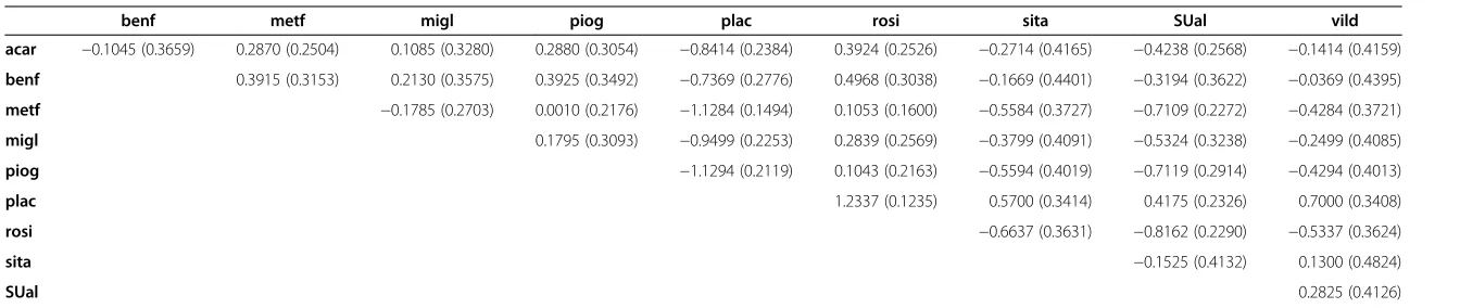
Table 8 Pairwise differences of the ten treatment means

benf metf migl piog plac rosi sita SUal vild

acar −0.1045 (0.3659) 0.2870 (0.2504) 0.1085 (0.3280) 0.2880 (0.3054) −0.8414 (0.2384) 0.3924 (0.2526) −0.2714 (0.4165) −0.4238 (0.2568) −0.1414 (0.4159)

benf 0.3915 (0.3153) 0.2130 (0.3575) 0.3925 (0.3492) −0.7369 (0.2776) 0.4968 (0.3038) −0.1669 (0.4401) −0.3194 (0.3622) −0.0369 (0.4395)

metf −0.1785 (0.2703) 0.0010 (0.2176) −1.1284 (0.1494) 0.1053 (0.1600) −0.5584 (0.3727) −0.7109 (0.2272) −0.4284 (0.3721)

migl 0.1795 (0.3093) −0.9499 (0.2253) 0.2839 (0.2569) −0.3799 (0.4091) −0.5324 (0.3238) −0.2499 (0.4085)

piog −1.1294 (0.2119) 0.1043 (0.2163) −0.5594 (0.4019) −0.7119 (0.2914) −0.4294 (0.4013)

plac 1.2337 (0.1235) 0.5700 (0.3414) 0.4175 (0.2326) 0.7000 (0.3408)

rosi −0.6637 (0.3631) −0.8162 (0.2290) −0.5337 (0.3624)

sita −0.1525 (0.4132) 0.1300 (0.4824)

SUal 0.2825 (0.4126)

Means for the diabetes example of Senn et al. [7] computed from model (2), dropping the design × treatment interaction (G.T) and modelling heterogeneity (G.S.T) as random. Table reports pairwise mean differences (and associated standard errors).

Medical

Research

Method

ology

2014,

14

:61

Page

8

o

f

9

ntral.com/1

estimated mean, but this is not significantly different from the other treatments outperforming the placebo.

In order to emphasize that the ANOVA implementa-tion also yields estimates of pairwise treatment contrasts and the associated standard errors, as does the baseline contrast implementation, we report these statistics in Table 8. This information is part of the standard output of mixed model packages, but is not convenient for rou-tine reporting in case of a larger number of treatments. The table of treatment means and the associated letter display provide a more compact summary of the net-work meta-analysis.

Discussion and conclusions

This paper has illustrated how a factorial ANOVA ap-proach can be used to perform NMA and to locate in-consistency in a given network. It was shown in Piepho et al. [6] that this analysis is either fully equivalent (summary measures, normal response in case of individual patient data) or very similar (individual patient data with non-normal responses and non-identity link functions in a GL(M)M framework) to the more commonly used ap-proach to meta-analysis based on baseline contrasts. We think that the ANOVA approach has some practical advantages. Interpretation of results is facilitated by the focus onttreatment means rather than ont(t−1)/2 pair-wise contrasts. Standard procedures for multiple compari-son of treatment means further aid the communication of results. Also, the approach may be appealing to those fa-miliar with ANOVA of factorial experiments. It has been demonstrated that standard diagnostic procedures for lin-ear models can be used to identify influential designs in the network and to detect sources of inconsistency. The results obtained for the diabetes example agree very closely with those obtained using recently proposed proce-dures based on a baseline-contrast approach [1]. We hope that this paper will help to popularize the ANOVA ap-proach as a viable and easy-to-use apap-proach to NMA.

Additional file

Additional file 1:Contains all SAS code that was used to obtain the results presented in this paper.

Competing interests

The author declares that there are no competing interests.

Received: 8 February 2014 Accepted: 9 April 2014 Published: 10 May 2014

References

1. Krahn U, Binder H, König J:A graphical tool for locating inconsistency in network meta-analysis.BMC Med Res Methodol2013,13:35.

2. Donegan S, Williamson P, D’Allesandro U, Smith CT:Assessing key assumptions of network meta-analysis: a review of methods.Res Synth Meth2013,4(4):291–323.

3. Lu G, Ades AE:Combining direct and indirect evidence in mixed treatment comparisons.Stat Med2004,23:3105-3124.

4. Higgins JPT, Jackson D, Barrett JK, Lu G, Ades AE, White IR:Consistency and inconsistency in network meta-analysis: concepts and models for multi-arm studies.Res Synth Meth2012,3:98–110.

5. White IR, Barrett JK, Jackson D, Higgins JPT:Consistency and inconsistency in network meta-analysis: model estimation using multivariate meta-regression.Res Synth Meth2012,3:111–125.

6. Piepho HP, Williams ER, Madden LV:The use of two-way mixed models in multi-treatment meta-analysis.Biometrics2012,68:1269–1277.

7. Senn S, Gavini F, Magrez D, Scheen A:Issues in performing network meta-analysis.Stat Methods Med Res2013,22(2):169–189.

8. Searle SR, Casella G, McCulloch CE:Variance Components. New York: John Wiley & Sons; 1992.

9. Wilkinson GN, Rogers CE:Symbolic description of factorial models for analysis of variance.Appl Stat1973,22:392–399.

10. McCullagh P, Nelder JA:Generalized Linear Models.2nd edition. London: Chapman & Hall; 1989.

11. Piepho HP, Büchse A, Richter C:A mixed modelling approach to randomized experiments with repeated measures.J Agron Crop Sci 2004,190:230–247.

12. Lu G, Welton NJ, Higgins JPT, White IR, Ades AE:Linear inference for mixed treatment comparison meta-analysis: A two-stage approach.Res Synth Meth2011,2:43–60.

13. Möhring J, Piepho HP:Comparison of weighting in two-stage analyses of series of experiments.Crop Sci2009,49:1977–1988.

14. Piepho HP, Möhring J, Schulz-Streeck T, Ogutu JO:A stage-wise approach for analysis of multi-environment trials.Biom J2012,54:844–860. 15. Whitehead A:Meta-Analysis of Controlled Clinical Trials.New York: Wiley &

Sons; 2002.

16. Nelder JA:Linear models: back to basics.Stat Comput1994,4:221–234. 17. Kenward MG, Roger JH:Small sample inference for fixed effects from

restricted maximum likelihood.Biometrics1997,53:983–997. 18. Belsley DA, Kuh E, Welsch RE:Regression Diagnostics; Identifying Influential

Data and Sources of Collinearity.New York: John Wiley & Sons; 1980. 19. Cook RD, Weisberg S:Residuals and Influence in Regression.New York:

Chapman and Hall; 1982.

20. Edwards D, Berry JJ:The efficiency of simulation-based multiple comparisons.Biometrics1987,43:913–928.

21. Piepho HP:A SAS macro for generating letter displays of pairwise mean comparisons.Commun Biometry Crop Sci2012,7:4–13.

doi:10.1186/1471-2288-14-61

Cite this article as:Piepho:Network-meta analysis made easy: detection of inconsistency using factorial analysis-of-variance models.BMC Medical Research Methodology201414:61.

Submit your next manuscript to BioMed Central and take full advantage of:

• Convenient online submission

• Thorough peer review

• No space constraints or color figure charges

• Immediate publication on acceptance

• Inclusion in PubMed, CAS, Scopus and Google Scholar

• Research which is freely available for redistribution