Max Planck Institute for Demographic Research Konrad-Zuse Str. 1, D-18057 Rostock·GERMANY www.demographic-research.org
DEMOGRAPHIC RESEARCH
VOLUME 24, ARTICLE 19, PAGES 455-468
PUBLISHED 15 MARCH 2011
http://www.demographic-research.org/Volumes/Vol24/19/ DOI: 10.4054/DemRes.2011.24.19
Formal Relationships 13
Linking period and cohort life-expectancy
lin-ear increases in Gompertz proportional
haz-ards models
Trifon I. Missov
Adam Lenart
This article is part of the Special Collection “Formal Relationships”. Guest Editors are Joshua R. Goldstein and James W. Vaupel.
c
°2011 Trifon I. Missov & Adam Lenart.
2 Proof of the relationship 456
3 History and related results 458
4 Applications 464
5 Acknowledgements 466
Linking period and cohort life-expectancy linear increases in
Gompertz proportional hazards models
Trifon I. Missov1
Adam Lenart2
Abstract
In a Gompertz mortality model with constant yearly improvements at all ages, linear increases in period life expectancy correspond to linear increases in the respective cohort life expectancy. The link between the two measures can be given by a simple approximate relationship.
1. Relationship
Suppose the mortality schedule of a population is described by
(1) µ(x, y) =e−ρya0ebx
on a period basis, which corresponds to
(2) µC(x, y) =e−ρya
0e(b−ρ)x
on a cohort basis, i.e., by a Gompertz hazard that decreases with timeyat a relative rate
ρat all agesxsimultaneously. Denote byeP
0(y)andeC0(y)the period and cohort life
expectancy iny. Vaupel (1986) proved that (1) results in a linearly increasingeP
0(y)with
an approximate slopeρ/b. We will prove that (2) implies linear increase ineC
0(y), too.
Moreover, fory→ ∞
(3) e
C 0(y)
eP 0(y)
−→ 1
1−e˙P 0(y)
and
(4) e˙C
0(y)−→ ˙
eP 0(y) 1−e˙P
0(y)
,
wheree˙P
0(y) =deP0(y)/dyande˙C0(y) =deC0(y)/dy.
2. Proof of the relationship
The number of years lived in the nextnby those who have survived to agexin yearyis
(5) L(x, n, y) = x+nZ
x
`(v, y)dv,
where
(6) `(x, y) = exp
− x Z 0
µ(v, y)dv
Substituting (1) and (6) into (5), assuming`(0, y) = 1, setting x = 0and letting
n→+∞, we get the following expression for period life expectancy at birth:
(7) eP
0(y) = 1
b exp
na
0
b e −ρyoE
1
³a
0
b e −ρy´,
where
(8) E1(z) =
∞
Z
z
e−t
t dt
is the exponential integral. A relationship, based on (2) and similar to (7), holds foreC 0(y),
as well:
(9) eC0(y) =
1
b−ρ exp
½
a0
b−ρe −ρy
¾
E1
µ
a0
b−ρe −ρy
.
The limit ofeC
0(y)/eP0(y)fory → ∞can be represented as
(10) lim
y→∞ eC
0(y)
eP 0(y)
= b
b−ρ·ylim→∞exp
½
−a0ρ
b(b−ρ)e
−ρy ¾ · lim y→∞ E1 ¡a 0
b e−ρy
¢
E1
³
a0
b−ρe−ρy
´.
The first limit on the right-hand side of (10) is equal to 1. The arguments of both ex-ponential integrals in the second limit tend to0fory → ∞. This implies that both the numerator and the denominator will tend to+∞as
(11) E1(z) =−γ−lnz−
∞
X
n=1
zn
n·n!
(see, for example, Abramowitz and Stegun 1964, 229), whereγ ≈ 0.577is the Euler-Mascheroni constant. Applying L’Hôpital’s rule yields
(12) lim
y→∞ E1
¡a 0
b e−ρy
¢
E1
³
a0
b−ρe−ρy
´ = lim y→∞exp
½
a0ρ
b(b−ρ)e
−ρy
¾
= 1
As a result, fory→ ∞
(13) e
C 0(y)
eP 0(y)
−→ b
b−ρ =
1 1−ρb =
1 1−e˙P
0(y)
Finally, differentiating (9) with respect toy, we get
˙
eC 0(y) =
ρ b−ρ
µ
exp
½
− 2a0
b−ρe −ρy
¾
+e−ρya 0ec0(y)
,
(14)
which implies fory→ ∞
˙
eC0(y)−→
ρ b−ρ =
ρ/b
1−ρ/b =
˙
eP 0(y) 1−e˙P
0(y)
(15)
Q.E.D.
3. History and related results
Linearly increasing record period life expectancy from 1840 to present was detected by Oeppen and Vaupel (2002). One of the possible models that yields constant increase per time unit is (1), introduced by Vaupel (1986). Goldstein and Wachter (2006) discussed the latter as a special case of Linear Shift Models (ρ/b = r), under which the hazard rate at every agexin yearyis given by the hazard rate at a younger agex−ry,r >0,
y years earlier: µ(x, y) = µ(x−ry,0). Wilmoth (2005) discussed the relationship between period and cohort mortality by comparing different mean life span measures in general model settings. Without specifying any functional interrelationship, Schoen and Canudas-Romo (2005) compare period and cohort life expectancy in the Gompertz proportional hazards framework with different shapesexp{−f(y)}of mortality progress over timey, includingf(y) = exp{−ry}, specified in (1). Canudas-Romo and Schoen (2005) study a Siler model with two different (constant) rates of mortality decline: one for infant and one for non-infant mortality. This model converges with time to (1) as levels of and improvements in infant mortality become negligibly small. Canudas-Romo and Schoen (2005) quantify the gaps and lags between period and cohort life expectancy over time in terms of the model parameters.
In this paper, within the framework of Gompertz proportional hazards (1), we express in a simple functional form the relationship between period and cohort life expectancy as well as between their (constant) rates of change. The two relationships are approx-imateanddo not depend on model parameters as it is the case in Canudas-Romo and Schoen (2005). Eq. (13) suggests that we can link period to cohort life expectancy by the following approximation
(16) eC
0(y)≈
eP 0(y) 1−e˙P
0(y)
whereas (15) implies that
(17) e˙C0(y)≈
˙
eP 0(y) 1−e˙P
0(y)
.
Note that fory→ ∞
exp
½
−a0ρ
b(b−ρ)e
−ρy
¾
= 1− a0ρ
b(b−ρ)e
−ρy+o(e−ρy)
and, following (11),
E1
¡a 0
b e−ρy
¢
E1
³
a0
b−ρe−ρy
´ = 1 +E1
¡a 0
b e−ρy
¢
−E1
³
a0
b−ρe−ρy
´
E1
³
a0
b−ρe−ρy
´
= 1 + lnb−ln(b−ρ) + a0ρ
b(b−ρ)e−ρy+o(e−ρy)
−γ−lna+ lnb+ρy− a0
b−ρe−ρy+o(e−ρy)
,
which implies that fora0 = 0.00001,b = 0.14, andρ= 0.027, formula (16)
overesti-mateseC
0(y)by2.12%-2.39%fory = 1,2, . . . ,100. Relationship (16) is sensitive with
respect to mortality progress. For instance, if ρ = 0.01, keeping all other parameters as before, we get an overestimate by0.7%-0.8%. Lowera0 and higherb increase the
accuracy in (16).
Relationship (17), though underestimating cohort life-expectancy increase, is much more accurate that (16). Note that fory→ ∞
˙
eC0 =
ρ b−ρ
µ
1 +a0e−ρy
µ
− 2
b−ρ−γ−lna+ lnb+ρy
+o(e−ρy)
Fora0 = 0.00001,b = 0.14, andρ= 0.027, the error in formula (17) is only between 4.05×10⁻⁶and8.47×10−5fory= 1,2, . . . ,100.
Formulae (16) and (17) provide a simple approximate relationship between eP 0(y)
andeC
0(y), as well as their rates of change. The two major assumptions under which this
result has been derived are: 1) the same yearly mortality improvement at all ages, 2) the Gompertz assumption about the baseline hazard.
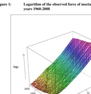
Figure 1: Logarithm of the observed force of mortality in Japan, ages 30-95, years 1960-2008
Fig. 1 shows clearly the significance of age-invariant period effects, especially at older ages where the force of mortality is increasingly Gompertz-like. Only one significant cohort effect can be seen for the cohorts born during the Second World War.
the observed rate of mortality change as
ρ(x, y+ 1) =−logµ(x, y+ 1)
µ(x, y) ,
and plotting it in Fig. 2, using again the Japanese data, we do not observe any particular age or period dependent pattern. The rate of mortality change appears rather to be a cloud centered around the mean value0.027. Life-expectancy increase in Japan has obviously not been exactly the same each year: there have been years of decrease followed by years of fast increase (negative and very highρvalues, respectively). Nevertheless a constantρ
is a good approximation to the observed mortality processes. The orange points on Fig. 2 show the interval of one standard deviation distance from the mean. It encompasses72%
of the data. The purple points (two standard deviations distance from the mean) and the orange points constitute together95%of the observed mortality changes.
Figure 2: Observed rate of mortality change in Japan, ages 30-95, years 1960-2008
Notes:Orange band designates theρvalues that fall into the mean±standard deviation. Theρvalues in the purple band are in the mean±two standard deviations interval.
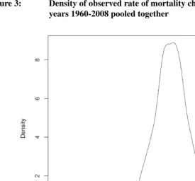
Fig. 3 shows the density estimate for the observed mortality change in Japan. As the rates are tightly packed around the mean, they corroborate the notion of age and time-invariant mortality change.
Figure 3: Density of observed rate of mortality change in Japan, ages 30-95, years 1960-2008 pooled together
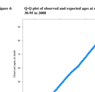
Figure 4: Q-Q plot of observed and expected ages at death for Japanese ages 30-95 in 2008
We derived (16) by using (7). The latter can be used to calculate life expectancy gains
GLE(x, y)at every agexin each yeary:
GLE(x, y) = de0(y)
dy = a0ρ
b e
−ρy(ebx−1) expn−a0
b e
−ρy(ebx−1)o.
(18)
Moreover, the age at which the maximal gains ineP
0(y)occur can be easily calculated as
x∗(y) = dGLE(x, y)
dx =
ln(b+e−ρya0) +ρy−lna 0
b .
Note that the agex∗(y)at maximal gains in life expectancy shifts almost uniformly
(y→ ∞) over time at a pace of
dx∗(y) dy =
ρ b.
(20)
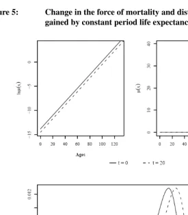
Thus the shift ofx∗(y)by periods (see Fig. 5) asymptotically (y→ ∞) equals the rate of
change in life expectancy at birth.
4. Applications
A proportionally changing force of mortality leads to a linearly shifting distribution of person-years gained by periods. In case of cohorts, this linear shift expands over time. Based on this relationship, cohort life expectancy at birth can be represented in terms of period life expectancy at birth and its derivative. A similar representation applies to the rate of change in cohort life expectancy at birth.
Relationships (16) and (17) provide an approximate estimate of how period gains in life expectancy are transformed on a cohort basis. Consider individuals that were born in
2010in a country with a period life expectancy at birth equal to80years. In this country, assume that (i) there is a constant2.5-year increase in life expectancy per decade (as in Oeppen and Vaupel 2002) and (ii) the force of mortality follows a Gompertz curve with constant yearly deceleration rateρ. In a period perspective, this would mean that during their childhood and young adulthood these individuals gain additional six hours of life every day (Vaupel 2009, 352). Throughout the life course this gain shrinks because there are less remaining years, in which mortality can improve. In order to claim that individu-als gain six hours a day in their infancy, one has to assume that they will experience the same probability of death, when they turn ten in2020, as the one for a10-year-old child in2010. Similarly, when they turn80in2090, they would have the same probability to die as a80-year-old person in2010. This assumption should hold on every day (or birth-day, depending on the measurement units) of their life. However, within our assumptions, mortality improves in such a way that individuals aged80in2090would have the same probability to die as a60-year-old person in2010.
In a cohort view, when we account for the ever changing mortality regime, we can see that these life expectancy gains are not negligible. Individuals in this country will have a (cohort) life expectancy of103.92years. If we do not correct for overestimation, our result will be 80
1−0.25 = 106.67years. Individuals born ten years later will have life
expectancy, which will be higher by 2.5
1−0.25 = 3.33years. Thus2.5-year life expectancy
Fig. 6 shows an example of changes in person-years lived in an age interval between two consecutive periods. Using the data from the Human Mortality Database, we chose Japanese females for demonstration. As life expectancy at birth augmentation over time is not constant even in Japan, we drew person-years-lived changes from one period to another to the same scale and removed six years when life expectancy at birth was lower than in the previous year. The resulting age distribution of person-years gained and the movement of the curve resembles the one predicted by the model (see Fig. 5).
Figure 6: Distribution by ages of person-years gained
Life expectancy gains result from the continuous linear shift to older ages in the distri-bution of person-years gained. Gompertz proportional hazards models stipulate reduction in the late middle-age and old-age mortality. Mortality of oldest-old, though, stays un-modified. However, as time advances, older and older ages benefit more from mortality reduction.
5. Acknowledgements
References
Abramowitz, M. and Stegun, I. (1964). Handbook of Mathematical Functions with For-mulas, Graphs, and Mathematical Tables. New York: Dover.
Bongaarts, J. and Feeney, G. (2003). Estimating mean lifetime. Proceedings of the Na-tional Academy of Sciences100(23): 13127–13133.doi:10.1073/pnas.2035060100. Canudas-Romo, V. and Schoen, R. (2005). Age-specific contributions to changes
in the period and cohort life exectancy. Demographic Research 13(3): 63–82. doi:10.4054/DemRes.2005.13.3.
Goldstein, J. and Wachter, K. (2006). Relationships between period and co-hort life expectancy: Gaps and lags. Population Studies 60(3): 257–269. doi:10.1080/00324720600895876.
Kannisto, V. (1994). Development of Oldest-Old Mortality, 1950-1990. Odense Mono-graphs on Population Aging, 1. Odense: Odense University Press.
Keyfitz, N. and Caswell, H. (2005). Applied Mathematical Demography. Statistics for Biology and Health. Springer.
Oeppen, J. and Vaupel, J. (2002). Broken limits to life expectancy. Science296(5570): 1029–1031.doi:10.1126/science.1069675.
Schoen, R. and Canudas-Romo, V. (2005). Changing mortality and average cohort life expectancy.Demographic Research13(5): 117–142. doi:10.4054/DemRes.2005.13.5. Tuljapurkar, S., Li, N., and Boe, C. (2000). A universal pattern of mortality decline in the
G7 countries.Nature405(6788): 789–792.doi:10.1038/35015561.
Vaupel, J. (1986). How change in age-specific mortality affects life expectancy. Popula-tion Studies40(1): 147–157.doi:10.1080/0032472031000141896.
Vaupel, J. (2009). Lively questions for demographers about death at older ages. Population and Development Review 35(2): 347–356. doi:10.1111/j.1728-4457.2009.00281.x.