in the population sciences published by the Max Planck Institute for Demographic Research Konrad-Zuse Str. 1, D-18057 Rostock · GERMANY www.demographic-research.org
DEMOGRAPHIC RESEARCH
VOLUME 14, ARTICLE 2, PAGES 27-46
PUBLISHED 25 JANUARY 2006
http://www.demographic-research.org/Volumes/Vol14/2/ DOI: 10.4054/DemRes.2006.14.2
Research Article
Increments to life and mortality tempo
2 Empirical results: Swedish females, 1751-2002 31
3 Time-continuous cohort-indexed increments to life 34
4 Time-continuous period-indexed increments to life 35
5 Relation between cohort and period increments to life 36
6 Robustness of the Bongaarts-Feeney Tempo Adjustment Formula 41
7 Increments to life and mortality tempo: mixed models 43
8 Conclusion 44
9 Acknowledgements 44
Increments to life and mortality tempo
Griffith Feeney 1
Abstract
This paper introduces and develops the idea of “increments to life.” Increments to life are roughly analogous to forces of mortality: they are quantities specified for each age and time by a mathematical function of two variables that may be used to describe, analyze and model changing length of life in populations.
The rationale is three-fold. First, I wanted a general mathematical representation of Bongaart’s “life extension” pill (Bongaarts and Feeney 2003) allowing for continuous variation in age and time. This is accomplished in sections 3-5, to which sections 1-2 are preliminaries. It turned out to be a good deal more difficult than I expected, partly on account of the mathematics, but mostly because it requires thinking in very unaccustomed ways.
Second, I wanted a means of assessing the robustness of the Bongaarts-Feeney mortality tempo adjustment formula (Bongaarts and Feeney 2003) against variations in increments to life by age. Section 6 shows how the increments to life mathematics accomplishes this with an application to the Swedish data used in Bongaarts and Feeney (2003). In this application, at least, the Bongaarts-Feeney adjustment is robust.
1. Time-discrete increments to life
Figure 1 shows cohort survival for two birth cohorts of Swedish females. In the usual way of thinking, the survival curve for the later cohort has moved up because risks of death have declined, but we might equally well think of the curve for the later cohort as having moved to the right as a result of the prolongation of life.
To quantify this idea, consider the earlier cohort, choose a particular age (x = 50 years, say) and consider the horizontal distance between the two survival curves at the corresponding survival proportion, c(50, )t1 =0.6666(Figure 1), t denoting the time 1
of birth of the earlier cohort. To calculate this distance we need to know the age to which this proportion of persons survive in the later cohort. Interpolating on the values for the later cohort we find this age to be 60.65 years, i.e.,c(60.65, )t2 =0.6666. The
horizontal distance between the two curves at the ordinate value
1 2
(50, ) (60.65, ) 0.6666
c t = c t =
is thus t t1,2(50) 10.65 c
λ = years.
The difference between any two survival curves may be described as the collection of all such horizontal distances. These “increments to life” are plotted in Figure 2. The increment for any given age represents “how much longer” persons in the second cohort live in a rather special and formal sense. The persons in the second cohort who survive to age t t1,2( )
c
x+λ x live ,
( )
t n c x
λ years longer than the persons in the first cohort who survive to age x. Their advantage is retrospective, however, not prospective. The increment to life for older ages may be smaller, zero or negative.
The area under the increments to life curve is the difference between the areas under the survival curves. Since the area under the survival curves gives the expectation of life at birth for the two cohorts, we have the following decomposition of the difference between the expectations of life at birth in the two cohorts in terms of the increments to life values,
1,2
0 2 0 1 1
0
( ) ( ) t t ( ) ( , )
c c
c c
e t −e t = −
∫
∞λ x d x t (1)Figure 1: Survivorship for Swedish Female Cohorts of 1890 and 1900
0 20 40 60 80 100
0
.0
0
.2
0
.4
0
.6
0
.8
1
.0
Age
P
rop
or
tio
n
S
u
rv
iv
in
g
Age = 50 Prop = 0.6666
Figure 2: Time Discrete Increments to Life for Swedish Female Cohorts of 1890 and 1900
0 20 40 60 80 100
0
2468
1
0
1
2
1
4
Age
In
c
rem
ent
t
o
Li
fe
Age = 50
2. Empirical results: Swedish females, 1751-2002
Increments to life by single years of age may be calculated for successive pairs of annual birth cohorts for Swedish females using the data provided in the Human Mortality Database (http://www.mortality.org). The database provides period life tables by single years of age to age 110 years for Sweden for (as of September 2004) 252 years, from 1751 through 2002. The q values from these tables may be used to x
compute cumulative cohort survival for the birth cohorts of persons born at the beginning of each calendar year. Applying the calculation of the preceding section to each successive pair of cohorts gives increments to life by single years of age for successive pairs of cohorts. These values may be arranged in a table in which rows correspond to single years of age and columns to pairs of adjacent birth cohorts and therefore to calendar years.
Figure 3: Time-Continuous Cohort Increments to Life, Swedish Females, Average over Cohorts of 1751-1760
0 20 40 60 80 100
-0
.8
-0
.6
-0
.4
-0
.2
0
.0
0
.2
0
.4
Age
In
c
re
m
en
t t
o
Li
Figure 4: Time-Continuous Cohort Increments to Life, Swedish Females, Average over Cohorts of 1891-1900
0 20 40 60 80 100
0.
0
0
.5
1.
0
1
.5
Age
In
c
re
m
e
n
t to
L
if
3. Time-continuous cohort-indexed increments to life
Let c( , )x t denote the proportion of persons surviving to age x in the cohort of persons born at time t . These values define a two-dimensional surface over the age-time plane of the Lexis diagram. This surface may be described by its contour lines, the lines on the age-time plane along which proportions surviving are constant. If length of life is constant, these contour lines will be straight lines parallel to the time axis. If length of life is increasing (decreasing), they will move to higher (lower) ages. The assumption that the population age distribution defined by c( , )x t shifts to uniformly to higher ages (Bongaarts and Feeney 2002:16) is equivalent to the assumption that the rate of change of the contour lines with respect to age at any given time is invariant with respect to age.
Let the rate of change with respect to age of the contour line passing through the point ( , )x t be ( , )λ x t . The directional derivative of the surface defined by c( , )x t in the direction ( ( , ),1)λ x t equals zero because the value of c( , )x t does not change on the contour line. We therefore have
( , ) ( , )
( , ) 0
c c
c
x t x t
x t
x λ t
∂ +∂ =
∂ ∂
, (2)
where the constant factor in the definition of the directional derivative may be ignored since the value is zero. Formula (2) is equivalent to
( , ) ( , ) ( , ) c c c x t t x t
x t x
λ = −∂ ∂
∂ ∂
, (3)
which may be taken as the formal definition of the time-continuous cohort-indexed increment to life λc( , )x t at age x and time t . The partial derivative in the denominator shows that empirical increments to life values will tend to be unstable over age intervals over which few deaths occur, since for these intervals ∂c( , )x t ∂x will be close to zero.
Dividing both sides of (2) by c( , )x t and rearranging terms gives
( , ) ( , ) ( , )
c x t x t r x t x
where µ( , )x t denotes the force of mortality at age x and time t and ( , )r x t denotes
the age-specific growth rate at age x and time t of the normalized population i ic( , ). This shows that values of the increments to life function vary inversely with the values of the force of mortality function for any given age and time.
The definition of increments to life by formula (3) supposes that the values ( , )
c x t
are given. If we assume instead that values λc( , )x t are given, formula (2) defines a partial differential equation that may be solved for the values c( , )x t given the boundary condition c( , 0)x forx>0.
4. Time-continuous period-indexed increments to life
Let p( , )x t denote the proportion of persons born at time t−x who survive to age
x
.From this definition and that of c( , )x t it follows immediately that
( , ) ( , )
p x t = c x t−x
and (5a)
( , ) ( , )
c x t = p x t+x
. (5b)
Compare Appendix 1 of Bongaarts and Feeney (1998), which states the same relation using slightly different notation. The subscripts refer to the cohort indexing of the preceding section and the period indexing of this section. Note that both p( , )x t and
( , )
c x t
are survival proportions for cohorts; the difference is only in the time reference.
The time-continuous increment to life may still be defined as the direction for which the directional derivative equals zero, but this direction must now be specified as a vector rather than as a scalar. The period version of formula (2) is
1 2
( , ) ( , )
( , ) ( , ) 0
p p
p p
x t x t
x t x t
x λ t λ
∂ ∂
+ =
∂ ∂
, (6)
where the vector ( 1( , ), 2( , )) p x t p x t
λ λ gives the direction of the tangent to the contour line at the point
(x,t)
. For consistency with the cohort formulation we may assume that2
( , )
p x t
λ assumes only the values 1+ and 1− , corresponding to movement forward and backward in time.
5. Relation between cohort and period increments to life
Figure 5 shows a Lexis diagram in which the diagonal line beginning at time t and ending at time t+ +1 λc represents the tangent line to the contour line that passes
through the point ( , )x t of the surface i ip( , ). The slope of this line is by definition the
period increment to lifeλp =λp( , )x t .
The corresponding rate of change between the cohorts born at times
t
−
x
andt− +x 1, represented by the dotted diagonal lines, isλc =λc( ,x t−x). From the similarity of the two right triangles,
( , ) ( , )
1 ( , )
c p
c x t x x t x
x t x
λ λ − = λ −
+ − , (7)
from which it follows that λp( , )x t →1 as λc( , )x t → ∞ and λp( , )x t → −∞
asλc( , )x t → −1. Values of λc( , )x t less than 1− correspond contour lines moving
Figure 5: Lexis Diagram Illustrating Relation Between Cohort and Period Increment to Life
Zeng Yi and Land (2002) prove a special case of (7) for a model in which cohort fertility, period fertility, the shape of the age-schedule of fertility and the rate of change in the mean age at childbearing are all constant over time.
To obtain a more general formula, observe that the partial derivatives in (6) may be expressed as
( , ) ( , ) ( , )
p x t c x t x c x t x
x x t
∂ ∂ − ∂ −
= −
∂ ∂ ∂
(8a)
x
x+ λc Age
t t+1 t+1+ λc
Time
t−x t−x+1
Birth cohort
1 λc
λc
1( , ) ( , ) /
( , ) / ( , ) /
c p
c c
x t x t x t
x t x x x t x t
λ = −∂ − ∂
∂ − ∂ − ∂ − ∂
(9a)
if λp2( , )x t = +1 and
1( , ) ( , ) /
( , ) / ( , ) /
c p
c c
x t x x
x t
x t x x x t x t
λ = ∂ − ∂
∂ − ∂ − ∂ − ∂
(9b)
ifλp2( , )x t = −1. Dividing the numerator and denominator on the right hand sides of (9)
gives
1( , ) ( , )
1 ( , )
c p
c
x t x x t
x t x
λ λ
λ
− =
+ − , λc( , )x t > −1, (10a)
when λp2( , )x t = +1 and
1( , ) ( , )
1 ( , )
c p
c
x t x x t
x t x
λ λ
λ
− −
=
+ − ,λc( , )x t < −1 (10b)
whenλ2p( , )x t = −1. Formula (10a) is the same as formula (7), but the graphical
approach leaves it unclear how to cope with the case in which λp2( , )x t = −1 or, equivalently,λc( , )x t < −1.
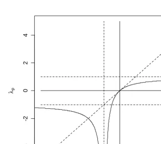
The relationship betweenλc( , )x t ,
1
( , )
p x t
λ and λ2p( , )x t is shown in Figure 6. The curve to the right of the vertical at λc( , )x t =1 shows the relation between λc( , )x t and
1
( , )
p x t
λ when λp2( , )x t = +1 and the curve to the left of this vertical shows this relation
whenλ2p( , )x t = −1.
The relation displayed in Figure 6 is curious indeed. Discussion of tempo effects in the demographic literature has generally (always, so far as I am aware) been limited to values of λc and λp fairly close to zero (roughly, say, the unit square centered on the
origin), and in this neighborhood the relationship is unremarkable. The Lexis diagram in Figure 5 shows that λp cannot exceed one, whereas λc may assume arbitrarily large
p
λ → −∞ as λ → −c 1 is rather less comfortable (though obviously, from (10a), this is what happens), since this suggests that tempo effects in this case can have arbitrarily large magnitude. In demographic terms (Lexis diagram in Figure 5), events in successive cohorts are shifting to younger ages in such a way as to pile up events on the vertical line at time t .
The portion of Figure 6 to the left of the vertical (dotted line) at
x
= −
1
is even more surprising. The idea that events occurring in successive cohorts may be moved to earlier ages so rapidly that the period effect is to “thin out” events and reduce period levels rather than to “bunching up” events and increase period levels has not, so far as I am aware, ever been considered in the demographic literature. Yet this is what happens whenλ <c 1. In demographic terms (Lexis diagram in Figure 5), events in subsequent cohorts are moved to earlier ages so rapidly that they occur earlier in time than events to earlier cohorts. The asymptotic approach to λp to the left of the vertical line (dotted) at1
x= − mirrors the asymptote on the other side, but with λc decelerating toward 1− . Of
course the value of λc is constrained on the left because events cannot be shifted to a
Figure 6: Relation Between Cohort and Period Increments to Life
-4 -2 0 2 4
-4
-2
0
2
4
6. Robustness of the Bongaarts-Feeney Tempo Adjustment Formula
The Bongaarts-Feeney mortality tempo adjustment formula (Bongaarts and Feeney 2002, 2003) is based on the “constant shape assumption,” which they show to be equivalent to the assumption that the normalized age distributions p( , )x t are translated uniformly up or down the age axis with changing time. This is equivalent to the assumption that period increments to life λp( , )x t are constant with respect to age
for each time t, λp( , )x t =λ( )t for all a. This suggests that tempo adjusted life
expectancy at birth may be calculated more generally by replacing ( )λ t by λp( , )x t in the Bongaarts-Feeney tempo adjustment formula (2003: formula 11, in whichλ = ∂( )t M t1( ) ∂t.
This adjustment may be applied to average of annual values of q for Swedish x
females for 1980-1995 with q set equal to zero for x x<30 years, the same Swedish
data used in Bongaarts and Feeney (2003). Values ofλp( , )x t are obtained by first
calculating λc( , )x t using formula (3) and then applying formula (10) to obtain values
ofλp( , )x t . The resulting period increments to life by age λp( , )x t are plotted in Figure
7, which suggests that they are reasonably close to constant with respect to age from about age 35 onward.
Calculation of a tempo-adjusted e using these values gives 79.5 years, as 0
compared with an unadjusted value of e0=81.0 years, for a tempo effect of
1.5
years.Figure 7: Time-Continuous Period Increments to Life, Swedish Females, 1980-1995 (qx = 0 for x < 30 years)
0.
0
0
0.
05
0
.10
0.
15
0.
20
Age
P
e
ri
o
d
I
n
c
re
m
e
n
t
to
L
if
e
7. Increments to life and mortality tempo: mixed models
What happens if the conditioning on survival to mid-adult ages is dropped and variable increments to life are substituted for the constant increment to life used in the Bongaarts-Feeney adjustment formula? The procedure described in the previous section gives in this case an expectation of life more than 5 years lower than the conventional expectation of life. The magnitude of the implied tempo effects is about three times larger than the tempo effects calculated by Bongaarts and Feeney.
The explanation for this discrepancy is evidently the age variation in increments to life shown Figures 3 and 4. The Bongaarts-Feeney mortality tempo adjustment is derived on the assumption that increments to life are constant with respect to age. When the survival function is conditional on survival to age 30 years, the Swedish increments to life 1980-1995 vary in a range of about±0.05, as shown in Figure 7. When the survival function is unconditional, increments are very far from constant. Figure 4 shows a variation of about±0.9. Conditioning on survival to age 30 has the effect of radically reducing the variability of increments to life by age.
Consistency with the Bongaarts-Feeney mortality tempo model therefore requires that increments to life be considered only for adult survival. The nature of mortality change at younger and older ages appears to be fundamentally different, so that the tempo model that makes sense at older ages does not make sense at younger ages.
So regarded, the Makeham defines a mixed model incorporating both forces of mortality and increments to life. Both components of the model could be generalized, to arrive at a more realistic model without changing the mixed nature of the model.
8. Conclusion
The study of mortality and length of life has been dominated by the concept of risks of death, to the point that mortality is sometimes regarded as being defined by age-specific death rates and the force of mortality function. Empirically, however, survival functions are the theoretical structure closest to the empirical data (migration may be handled with product limit survival functions), and changing survival functions give rise to and may be modeled by both forces of mortality and increments to life.
When we think in terms of risks of death, life times are a residual. How long we live reflects how successful we are in escaping various risks of death. When we think in terms of increments to life, deaths are the residual. Death is what happens when we run out of life. As pointed out by Vaupel and Yashin (1987), physicians and health personnel tend to think more in the latter terms than the former. They suggest also that the two perspectives are complementary rather than contradictory. A better understanding of this complementarity may usefully advance the study of changing mortality and length of life.
9. Acknowledgements
This work has been supported by the Population Council. For comments on earlier drafts of this paper I am grateful to John Bongaarts, to the participants in the Workshop
on Tempo Effects on Mortality (18-19 November, New York City), especially to Jutta
References
Bongaarts, John, and Griffith Feeney. 2002. How long do we live? Population
Development Review 28(1):13-29.
Bongaarts, John, and Griffith Feeney. 2003. Estimating mean lifetime. Proceedings of
the National Academy of Sciences 100(23):13127-13133.
Vaupel, James W., and Anatoli I. Yashin. 1987. Repeated resuscitation: How lifesaving alters life tables. Demography 4(1):123-135.