Tehran Stock Price Modeling and Forecasting Using Support Vector Regression (SVR) and Its Comparison with the Classic Model ARIMA

(1)

Tehran Stock Price Modeling and Forecasting Using

Support Vector Regression (SVR) and Its Comparison

with the Classic Model ARIMA

Saeed hajibabaei* Nematollah hajibabaei** Syed mohammad hoseini***

Somaye hajibabaei**** sajad hajibabaei*****

Received: 2013/04/16 Accepted: 2013/12/11

* MSc; Department of Art and Architecture, Hamedan Branch, Islamic Azad University, Hamedan, Iran(Corresponding Author)

** MSc Candidate; Department of MANAGMENT, Buin zahra Branch, Islamic Azad University, Buin zahra, Iran

*** MSc Candidate; Department of Art and MANAGMENT, malayer Branch, Islamic Azad University, malayer, Iran

**** MSc; Department of Accounting, Hamedan Branch, Islamic Azad University, Hamedan, Iran

***** MSc Candidate ; Department of Art and Architecture, Hamedan Branch, Islamic Azad University, Hamedan, Iran

Abstract

se of linear and non-linear models to predict the stock price has been paid attention to by investors, researchers and students of finance and investment companies, and organizations active in the field of stock. Timely forecasting stock price can help managers and investors to make better decisions. Nowadays, the use of non-linear methods in modeling and forecasting financial time series is quite common. In recent years, one of the new techniques of data mining with support vector regression (SVR) has had successful application in time series prediction. In this study, using support vector regression model, we examined the Tehran Stock prices and the predicted results were compared with ARIMA classic model. For this purpose, of the Tehran stock companies, 5 companies were selected during the years 2002 to 2012. Using benchmarks to evaluate the performance of MSE, MAE, NMSE these two methods were compared and the results (in the case of non-linear data) indicate the superiority of SVR model compared to the ARIMA model.

Keywords: stock investment, stock price forecasting, data mining, support vector regression, ARIMA models

(2)

2/ Tehran Stock Price Modeling and Forecasting Using Support Vector…

1- Introduction

Achieving the long-term and continuous economic growth demands optimal allocation of resources at the national economics level which is impossible to obtain without the help of financial markets, especially extensive capital market .In a healthy economy, the presence of a financial system plays a role in proper distribution of funds and financial resources.

Usually, the financial markets are defined as a system composed of individuals and institutions, instruments and procedures that are collecting savers all in one place. One of the most attractive financial markets in which asset management and decision making quality are of extremely importance is stock market. In this market, the correct decision making has even greater importance than in traditional markets like commodities market and to do suitable activities and create wealth, the power of prediction ,direction and pace of change are very important. Stock price forecasting is a popular and important topic in financial and academic studies

.

(Yue xo, 2012) Yet, the number of individuals having experience and talent to guess the direction of stock market is few .Therefore , the systems which can help to make a proper decision is very valued.

Predicting stock index is a major activity of financial firms and private investors. However, stock index prediction is regarded as a challenging task of the prediction problem since the stock market is a complex, evolutionary, and nonlinear dynamic system (Lu et al, 2011). Highly accurate interval forecasting of a stock price index is fundamental to successfully making a profit when making investment decisions, by providing a range of values rather than a point estimate. (xiong, 2013)

Support vector regression (SVR) has successfully solved prediction problems in many domains, including the stock market. (Hung, tsai, 2009). Support vector regression (SVR) has become a popular alternative in stock index forecasting tasks due to its generalization capability in obtaining a unique solution

.

(dai et al, 2013)

(3)

method, due to its outstanding properties such as simple geometric interpretation, reaching a general and unique solution is noticeable. Choosing best model in SVM model is equal to solving a quadratic programming problem, which leads to a unique and general solution. On the other hand, SVM can estimate the complex non-linear functions by applying a suitable core function and mapping the original data into a higher dimensional space. (Basak et al, 2007) due to these features, the use of genetic algorithm has become widespread as in predicting stock price in stock market. Also, one of the methods to predict stock price in market is mixed SVM-ARIMA model. (Ince and Trafalis, 2006)

2- Support Vector Machines for Regression Problems (SVR)

Based on Statistical Learning Theory, Support Vector Machine (SVM), was first developed by Vapnik( vapnik, 1998) Another version of SVM method for regression problems in year is called. support vector regression (SVR) (Vapnic, 1995) Application of support vector regression (SVR) could improve forecasting accuracy performance.(hong et al, 2013) The model produced by svc is only a subset of the training dependent sample .similarly , the produced model by the SVR is only a subset of training dependent samples because the loss function for model construction ignores the training data which are close to prediction model ( at ε distance from the prediction model) This is corresponding to using loss function ε- insensitive suggested by Vepnic and produces one sparse set of support vectors .

Overall, SVR acts to estimate the regression function as the following a. Estimate the regression function in a set of linear functions as

b X w X

f( )( ,( ))

b. Minimizes empirical risk with respect to loss function

ε

- insensitive c. Performs structural risk minimization principle to minimize the real risk in that it considers the structure of the set of linear functions (defined by norm of coefficients of linear functions) as follows

:

H1CH2C…CHkC…

Where Hk element of the structure is defined by the following inequality

:

k

C

w

||



(

,

)



||

2 (1)

(4)

4/ Tehran Stock Price Modeling and Forecasting Using Support Vector… 2-1- Linear Mode

Suppose we have the training data S= {(x1,y1), (x2,y2) , … , (xn, yn)} CRd×R in which n is the number of samples and Rd represents the input space . In SVR, our goal is to find a function f(x) which for all instances has ε values deiation from the real purpose of yi and is as smooth as possible. In other words, the errors that are less than ε are overlooked, but it will not accept errors greater than e. linear regression function in the input space can be estimated as follows:

x,w€Rd_{, b € R}

f(x)=(w,x)+b (2)

Smoothness of (2) means that we are looking for a model with minimal complexity. According to what was mentioned in the previous section, this is done with minimization of ||w||2. So the main problem can be written as follows: (smola, Scholkopf, 1998)

2

|| || 2 1

min w (3)

n 1,2,..., i , ε y b x w, n 1,2,...., i , ε b x w, y s.t. i i i i         (4)

Which is a quadratic optimization problem. The implicit assumption in (4) is that there really is a function f which can approximate all pairs (xi, yi) with accuracy ε. Or in other words, the above optimization problem can be solved. Sometimes it may happen that the relation (4) does not hold for all training samples. To deal with impossible constraints in the aboe optimization problem, we define the auxiliary variables of



_i*

,



_iso that they satisfy the following restrictions.

(5)

In which



i(*) refers to variables of



i

,



i *

and constants C> 0 is a balance between smoothness of f and empirical risk. For example, if C=∞, then the aim is to minimize the empirical risk regardless of the complexity of the model.

Figure 1. (a) auxiliary variables (b)



i

,



i *

are loss function

ε

- insensitive (a) Auxiliary variables (b)



i

,



i

*

are loss function

ε

- insensitive which is defined as follows:

























.

0 |

)

(

|

)

(

|

0 )

0 ,

|

)

(

max(|

))

(

x

f

y

x

f

y

x

f

y

X

f

y

L

In most cases, the above optimization problem is solved easily in its dual formulation. Using coefficient method of Lagrange, we have:



   

























n 1 i * i * i i i n 1 i i i * i i n 1 i i i i i n 1 i * i i 2

)

ξ

β

ξ

(β

b)

x

w,

y

ξ

(ε

α

b)

x

w,

y

ξ

(ε

α

)

ξ

(ξ

C

||

w

||

2

1 β)

α,

b,

L(w,

i i i i







*

,

*

,

Are Lagrange coefficients that satisfy the following conditions:

0 ,

,

*_i _i _i*



i

a





(6)

0 )

(

1 *







_

 i n i i

b

L

_

(7)

i

w

x

w

(

)

0 (

)

* 1 * 1 i n i i i n i i

L

_



 















(8) (*) (*) (*) (*)

(*) i i

0

i i

i

C

L

_

_

_

_

















(9)

By putting (7), (8) and (9) in the Lagrange function: we have



                               n i i i i n i i i n i n i i i i n i i i i i n i n i i i i i n i i i i i n i n i i i y y C C b b L 1 * 1 * 1 1 * 1 1 1 * * 1 * * 1 1 * ) ( ) ( ) , ( 2 1 ) ( ) ( ) ( ) ( ) ( , ) ( , 2 1 ) β , α , , (





























w w x w w w w _i

Thus, the optimization problem is obtained under the dual form

    



  j i x x, ) ( ) ( 2 1 * 1 1 * α

max

i i

n

i n

i

i   

 (10)

)

(

)

(

* 1 1 * i i n i i n i i

i



y













 







n i i i

t

s

1 *

0 )

(

.



(11)

]

,

0 [

,

_i*

C

i







Calculating the Lagrange coefficients from equation (11) and using equation (8), we can write f(x) as the following:



















n i i i

b

X

f

1 *

,

)

(

,

)

(

w

x



x

_i

x

(12)

As it can be seen, SVR algorithm is described in terms of the dot product between the data, and cwe not need to compute w explicitly to get f(x).

2-1-1 calculation b

To find f(x), w is required to be computed in addition to b. KKT conditions reflect the product of the dual variables and constraints must be zero.

0 )

,

(



_i



y

_i









b



i





w

x

i



(13)

0 )

,

(

* *













b

y

_i i

i





w

x

i

(7)

0 )

(

C





_i



_i



(15)

0 )

(

C





_i*



_i*



(16)

The above relationships provide some useful conclusions. First, only the samples

(

x

_i

,

y

_i

)

corresponding to



_i(*)



C

are outside e- insensitive interval. Also,



_i

,



_i*



0

means there is never a set of dual variables of



_i and



_i* which become zero simultaneously .for



_i(*)



(

0 ,

C

)

we have

0

(*)



i



and therefore the second factor in 13 and 14 must be zero and b can be computed.

)

,

0 (

,

a

C

y

b



_i





w

x

_i







_i



)

,

0 (

,

a

*

C

y

b



_i





w

x

i







_i



The relations (13) and (14) result that only samples with







|

)

(

|

f

x

_i

y

_i Lagrange coefficients may be nonzero. For samples with







|

)

(

|

f

x

_i

y

_i the second factor in (13) and (14) is non-zero, hence for KKT conditions to hold,



_i and



_i* must be zero.

The samples which have nonzero Lagrange coefficients are called support vectors. Due to this and the relations (8) and (12), to compute f (x) and w , we do not need all of xi, but only support vectors are involved in the calculation of w and f (x) . This property is called sparseness because the complexity of the model depends only on the number of support vectors.

2. Non -Linear mode

In SVR method when we cannot fit a linear regression function in input space to data, we can use a nonlinear mapping to transform data in to a space with greater dimension and the standard svr algorithm is applied in this new space. Thus, linear regression in the new space corresponds to nonlinear regression in the original input space.

As mentioned, the linear SVR algorithm is dependent on only dot product between data the nonlinear SVR algorithm only depends on the dot product.

Replacing the kernel function for dot product of





(

x

_i

),



(

x

_i

)



in new space with great dimension, the linear regression function is written as follows.

























n i j i i

i

x

b

(8)











n

i

i i

i

K

x

b

1

*

)

,

(

)

(



Using kernel functions instead of a dot product of, calculations are done. Using data from the original input space, without having to know the mapping. There are a variety of kernel functions the common of which are polynomials of RBF Gaussian, RBF exponential and tangent hyperbolic.

3- Introduction to ARIMA models

ARIMA model is a linear - stochastic time series model in econometrics which is used for stationary and no stationary time series .one of the methods for transformation of no stationary series into a stationary series is subtraction method .for the Prediction of model ARIMA (p, d, q) the methodology of Jenkins box is used that has four stages: identification, estimation, diagnostic control and prediction. (Brillinger, 1981; Chattfield, 1975; box, Jenkins, 1975)

ARIMA model is one of the most common methods of forecasting time series. In an ARIMA model, the future value of a variable is expressed as a linear combination of past values and past errors as follows:



















t t p t p t t t q t q

t

y

 0 1 1 2 2    1 1 2 2  (17)

Where yt is the actual value,

ε

t the random error at time t,

φ

i and

θ

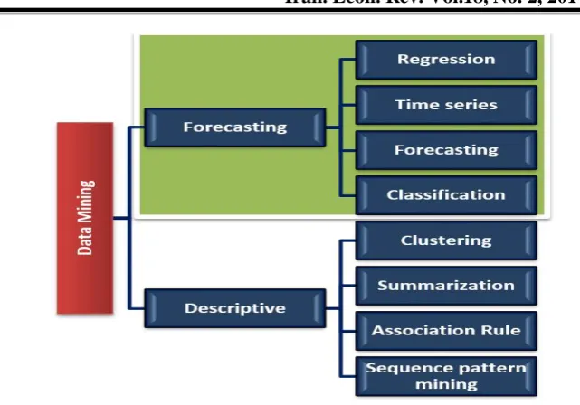
j coefficients and p and q are integers which are the ARIMA model orders. In these models, with the appropriate pre-processing methods, the data are processed. ARMA model is then selected. To determine the model order, autocorrelation function and data partial autocorrelation are used.

4- Data mining

(9)

Figure 2: Data Mining Techniques

5- Process Modeling and Implementation of SVR Algorithm

(10)

10/ Tehran Stock Price Modeling and Forecasting Using Support Vector…

5-1- Statistical Samples

According to SVM model, the value of the sample must be too high. Because of this, data were selected on a daily basis from the variables. In the SVM algorithm, every raw data sets divided into three sections. The first part, which comprises 60 percent of the data, is used as the training set to build the model. The second part comprising 30 percent of total data is called validation set used for selection of SVM model parameters and the remaining 10 percent is used as assessment of model accuracy. The table below shows how data are divided into three subsets of the training, validation and testing.

Table1: Separation of Data into Three Educational, Validation and Testing

Subsets TOTAL TEST VALIDATION TRAINING COMPANY 1795 95 550 1150 Ghadir 1497 97 400 1000 Khodro 1472 152 450 870 Roy 1198 98 350 750 Saipa 1963 163 600 1200 Setran

One of the steps of pre-processing time series data is using a moving window method. K window display is shown below.

n k

k

x

₁

,

₂

,

₃

,....

,

_₁

,

_₂

,...

The first input







n i i i

t

s

1 *

0 )

(

.



The second input

x

₂

,

x

₃

,....,

x

k₁

The third input

x

₃

,

x

₄

,....,

x

_k_₂ The last entry

x

n_{ }k1

,....,

k

n

To fix the remote point problem and prevent computational problems, it is better for data to be scaled in the interval [1, 0] or [+1, -1]. the following equation scales the data in the interval [0, 1]

min min 1

X

Y

ma i





(18)

(11)

5-2- Choosing the Parameters

Before implementation of SVR algorithm, it is needed to specify the type of kernel function parameters and the parameters



, and c. The accuracy of SVR models largely depends on the proper choice of kernel function parameters



and c. Each of the parameters influences the model complexity and accuracy of predictions.



Is defined as acceptable radius over deviations from the regression function such that an increase of



reduces the number of support vectors. On the other hand, parameter c makes a balance between experimental risk and complexity such that increasing c increases the importance of learning error compared to model complexity. SVR algorithm, with the application of an appropriate kernel function and mapping the data into a higher dimensional space, is able to find nonlinear regression functions. Proper choice of kernel function and its parameters plays an important role in the complexity and accuracy of SVR models.

regarding the nonlinear data, we use a Gaussian RBF kernel function as applied in most applications of time series prediction (tay and cao, 1992) and a grid search method is used to select the model parameters in that taking two parameters constant, the values of the parameters will change based on the lowest MSE in data validation to select the best parameter value. (Cao and tay, 2001)

The following table shows selected parameters for the five data sets:

Table 2: Selected Parameters for 5 Sets of Data from Ghadir , Khodro,

Roy, Saipa and Siman Tehran

ε с

γ

0.1 4900

0.75 GHADIR

0.00025 700

5 KHODRO

1 50000

1 ROY

0.03 7000

0.25 SAIPA

0.15 2000000

1.5 SETRAN

(12)

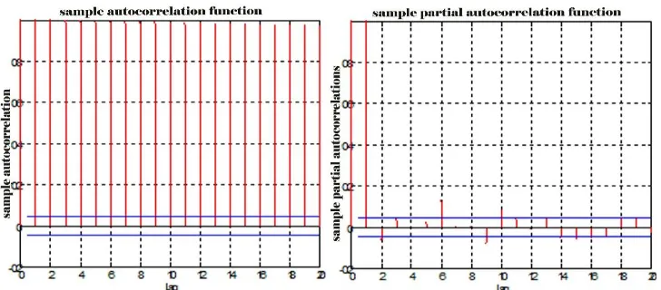
5-3- Autocorrelation and Partial Autocorrelation Functions

One of the Interpretation tools for identification of model is the autocorrelation and partial autocorrelation functions of time series which is presented and discussed.



         _n t t k n t k t t k k

x

c

r

1 1

0 ₍ ₎

) )(

(

and (19)

) , cov( ) , cov( ) 0 ( ) ( ) (

x

t t k t t k

k   

  

In which p (k) is the autocorrelation function and rk is autocorrelation coefficient                       1 1 2 1 1 1 1 2 1 1                k k k pk pk pk kk *   (20)

And _

kk is the partial autocorrelation function, pk is autocorrelation

(13)

Figure 4: Autocorrelation and Partial Autocorrelation Functions Data of

Ghadir Company

Figure 5: Autocorrelation and Partial Autocorrelation Functions Data of khodro Company

Figure 6: Autocorrelation and Partial autocorrelation functions data of roy

(14)

Saipa Company

Siman Company

5-4- Pre- Processing Methods for Time Series Data

Financial time series demands preprocessing techniques due to features such as non-stationary, noise and nonlinearity .depending on data type, different methods are used to preprocess. One of the conditions of ARIMA model is the stationary mode of the data (either in terms of mean and variance). If the variance of data is non-stationary, by stability transformation, variance and the mean become stationary through differential.

5-5 sustainability Transformations of Variance

(15)

(16)

Figure 9: Main Data of Siman Figure 10: Data of Tehran Siman

Tehran Company Company after Stabilization

In this company, regarding the fact that data variance is highly variable (over time), a logarithmic transformation was used to stabilize variance .after logarithmic transformation was used to stabilize the variance, it is observed that the data are non- stationary in the mean .to eliminate the problem , differential was used to make data stationary.

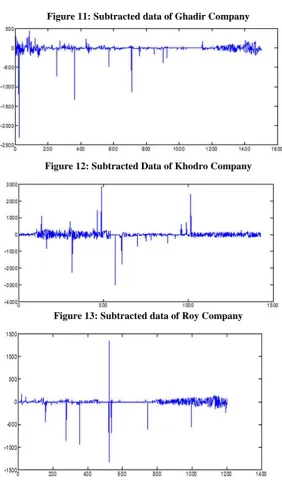
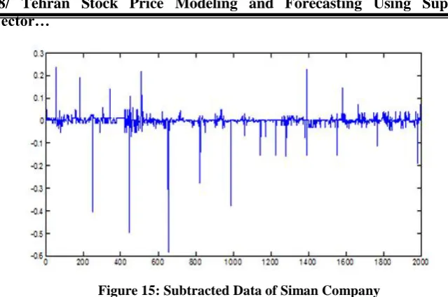
5-6- The Difference between Takings

One of the most common preprocessing techniques time series is differential used for making data stationary (on average). After taking the first difference of the time series, Original time series becomes:

X

Y

t





t



t1



t (t1,2,....,n1)

(17)

Figure 11: Subtracted data of Ghadir Company

Figure 12: Subtracted Data of Khodro Company

Figure 13: Subtracted data of Roy Company

(18)

Figure 15: Subtracted Data of Siman Company

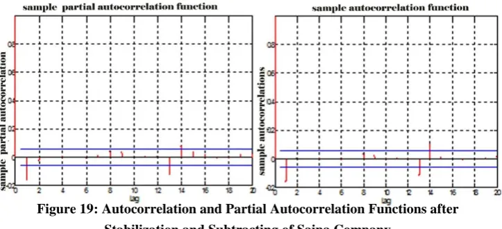
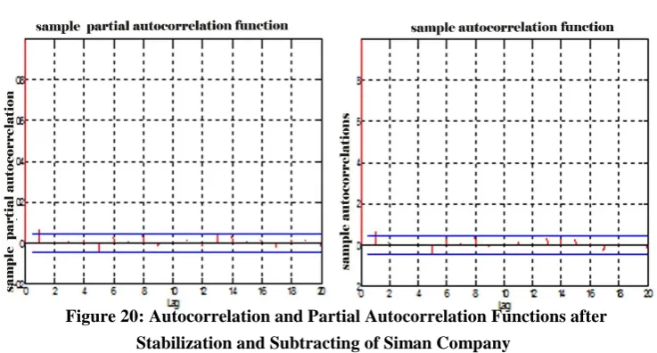
5-7- Autocorrelation and Partial Autocorrelation Functions after Stabilization and Subtracting

After stabilization, partial autocorrelation and autocorrelation functions for stationary data are re-plotted:

Figure 16: Autocorrelation and Partial Autocorrelation Functions after

(19)

Stabilization and Subtracting of Khodro Company

Stabilization and Subtracting of Roy Company

(20)

Stabilization and Subtracting of Siman Company

5-8- Detection of Model ARIMA (p, d, q)

Given the time-series graph and plotting the autocorrelation functions and partial autocorrelation, ARIMA (p, d, q) can be detected where d is the number of differentials and p and q are detectable with autocorrelation and partial autocorrelation. This means that the shape of the autocorrelation function plot after delay (q-p) tends to zero and the partial autocorrelation function of delay (p-q) tends towards zero.

(21)

5-9- Prediction of Stock Price of Companies Using SVR and Its Comparison

with Arima

Figure 21: Prediction of Stock Price of Ghadir Company Using SVR and Its Comparison with Arima

Figure 22: Prediction of Stock Price of KHODRO Company Using SVR and Its Comparison with Arima

(22)

Figure 24: Prediction of Stock Price of Saipa Company Using SVR and Its

Comparison with Arima

Figure 25: Prediction of Stock Price of Siman Company Using SVR and Its

5-10- performance evaluation criteria

(23)

Overall, the closer actual amount is to the value predicted by the model, more accurate the prediction model is. Therefore, the model quality is assessed by the expected error rate. In this regard, three factors mean square error (MSE), mean absolute error (MAE) and the normalized mean square error (NMSE) will be looked into.







l

t

p

a

t

_t

l

MSE

1

2

)

(

1 







l

t t

t

p

a

l

MAE

1

)

(

1



 



 l

t at a

l 1( )

2

1 1 2

 



 l

t at l a

1 1

In which

l

is the number of testing data, a the real value in time t and p is the predicted value in time t.

Table 3: Prediction of Stock Price of Ghadir Company Using SVR and Its

GHADIR MSE MAE NMSE

SVR 167284 142.2967 0.1717

ARIMA(1,1,1) 154.670 128.2211 0.1588

Table 4: Prediction of Stock Price of Khodro Company Using SVR and its

comparison with Arima

KHODRO MSE MAE NMSE

SVR 6959.18 66.6487 0.0278

ARIMA(1,1,1) 8659 74.9038 0.0345

Table 5: Prediction of Stock Price of Roy Company Using SVR and Its

ROY MSE MAE NMSE

SVR 8415.1 77.916 0.0358

ARIMA(1,1,1) 8806.5 81.5858 0.0374

Table 6: Prediction of Stock Price of SAIPA Company Using SVR and Its

SAIPA MSE MAE NMSE

 

 ( )

2

2 1

pt at l

(24)

SVR 7090.64 73.4283 0.0348

ARIMA(1,1,1) 7263.7 74.4982 0.0357

Table 7: Prediction of stock price of SIMAN company using SVR and its

comparison with Arima

SIMAN MSE MAE NMSE

SVM 3360.8 34.3946 0.0705

ARIMA(1,1,1) 3193.8 26.9102 0.067

Comparing the results predicted based on the criteria of MSE, MAE and NMSE in companies of Iran Khodro and Saipa indicates the superiority of the SVR method to ARIMA. But for Ghadir Investment Company and cement Tehran, ARIMA model forecasts better than SVR model. this is due to the fact that the data of these two companies are linear in some periods and for linear data , Arima model outperforms .Obviously, the model outperforms better in its own condition .For example ,in ARIMA models where the data are mostly linear, better results can be achieved.

6- Conclusions

Prediction of stock prices in the stock market is of utmost importance. Investors in stock market can gain profit if they can predict the trend of stock market regarding the changes in other markets such as exchange, gold and oil. In fact, when investors gain profit from the stock market, the market will provide life survival.

In recent years, the increase of computation power and data storage in different fields has brought about a necessary provision for new techniques and smart tools .data mining is a relatively young field originated from statistics, artificial intelligence and machine learning referring to extracting knowledge and information from big database.one of the most important applications of data mining is making prediction based on previous data done in different ways.

(25)

In this study, we compare the classical regression model with SVR and high performance of computing and the results indicate that the SVR model outperforms the other. Of course, this does not mean ignoring other methods, and each model has its own efficiency. But Tehran Stock market should take advantage of the different methods for the implementation experience of the other markets, such as the New York and japan Stock Exchange.

All can be concluded is that using mathematical model in estimating stock price is of great importance.

Among all kinds of time series data, forecasting financial time series, due to characteristics such as non-stationary, noise and non-linearity, is more difficult. In this study, the performance of SVR for financial time series prediction has been investigated. To do so, five sets of data related to ghadir ,irankhodro, saipa , siman Tehran and rooy toseh zanjan were selected.to select model parameters ,we used network search method.

After implementation SVR model, the predicted results the classical were compared with ARIMA model.

Given Autocorrelation and partial autocorrelation functions, Non-stationary data were specified and the need to stabilize the variance and the difference was felt. a random walk model was used for ghadir data and for irankhodro, Saipa , Tehran cement and rooy toseh ,we used an ARIMA model. And the predicted results were compared. based on the criteria of MAE, MSE and NMSE The results of this study showed that in the data of companies of irankhodro,toseh rooy ,and saipa , and Saipa, SVR model is better than the ARIMA, based on criteria of MSE MAE and NMSE . But given Tehran cement and Ghadir, ARIMA model showed more accurate predictions. Then selection the appropriate model from existing models is one of the most important factors in understanding the stock market.

As in most developed countries such as japan and USA, SVR and other mathematical models model are used to predict stock market, some suggestions are presented below to establish a robust system in stock market and improve the accuracy of SVR model.

1) Education of the investors in stock market for the use of mathematical models to predict the stock price

(26)

3) Finding a more accurate and faster method for selecting model parameters of SVR.

4) Combining SVR approach with other methods and using appropriate pre-processing methods to increase the accuracy of the model.

5) Finding new kernel functions to be applied in various data.

References

1- Basak, D. et al. (2007), Suort Vector Regression, Neural Information Processing- Letters and Reviews, 11, No. 10, 203-223.

2- Boser, E, Guyon, I, Vapnik, V, A training algorithm for optimal margin classifiers. In Haussler, David (editor); 5th Annual ACM Workshop on COLT, pages 144–152

3- Box G. E. P. and Jenkins G. M. (1976), Time Series Analysis: Forecasting and Control. Revised Edition. Holden-Day.

4- Brillinger. (1981), Time series Data Analysis and Theory Expanded Edition. McGraw-Hill. Inc. New York.

5- Cao, L. J.and Tay, F. E.H. (2001), Financial Forecasting using Support Vector Machines, Neural Comput Applict, 10, 184-192.

6- Cao , L. J. and Tay, F. E.H. (2003), Support Vector Machine with Adaptive Parameters in Financial Time Series Forecasting, IEEE Transactions on Neural Networks, vol. 14, No. 6, PP.1506-1518

7- Chattfield C. (1975), the Analysis of Time Series. An introduction. New York, Chapman and Hall.

8- Chen, W, Shih, j-y. (2006), Comparison of Support Vector Machines and Back Propagation Neural Networks in Forecasting the Six Major Asian Stock Markets, International Journal of Electronic Finance,. 1, No. 1, 49, 49-67.

9- Dai, W, shao, Y, lu, C, (2013), Incorporating feature selection method into support vector regression for stock index forecasting, Neural Computing and Applications, Volume 23, Issue 6, pp 1551-1561

10-Engle, R. (1982), Autoregressive Conditional Heteroskedasticity with Estimates of the Variance of United Kingdom Inflation, Economical, 50, Issue 4, 987-1008.

(27)

12-Feng pai, P, sheng lin, C, (2005), A hybrid ARIMA and support vector machines model in stock price forecasting, Omega, Volume 33, Issue 6, Pages 497–505

13-Han, J. and kamber, M, (2006), data mining concepts and techniques, second editition, Elsevier, morgan koufmann peblishers.

14-Hong, W, dong, Y, zhang, W, chen, L, Panigrahi, B, (2013), Cyclic electric load forecasting by seasonal SVR with chaotic genetic algorithm, International Journal of Electrical Power & Energy Systems, Volume 44, Issue 1, Pages 604–614

15-Hung, C, tsai, C, (2009), A hybrid SOFM-SVR with a filter-based feature selection for stock market forecasting, Expert Systems with Applications, Volume 36, Issue 2, Part 1, Pages 1529–1539

16-Ince, H. and Trafalis, T. B. (2006), A Hybrid Model for Exchange Rate Prediction, Decision Suort Systems, 42, 1054-1062.

17-Lu, C, wu, J, chiu, C, tsai, Y, (2011), Predicting Stock Index Using an Integrated Model of NLICA, SVR and PSO, Advances in Neural Networks, Volume 6677, pp 228-237

18-Smola, A. and Scholkopf, B. (1998), A Tutorial on Support Vector Regression, Technical Report NeuroCOLT NC-TR-98-030.

19-Tan, P. N., Steinbach, M. and Kumar, V. (2006). Introduction to Datamining. Pearson Education, Inc., Boston, MA.

20-Tay, F. E. H. and Cao, L. J. (2001), Application of Support Vector Machines in Financial Time Series Forecasting, The International Journal of Management Science, Omega, 29, PP. 309-317.

21-Vapnik, V. N. (1995), the Nature of Statistical Learning Theory, New York: Springer-Verlag.

22-Vapnik, V.N. (1998), Statistical Learning Theory. Wiley, New York. 23-Xiong, T, bao, Y, hu, Z, (2013), Multiple-output support vector regression with a firefly algorithm for interval-valued stock price index forecasting, Knowledge-Based Systems, Volume 55, Pages 87–100