An Artificial Neural Network Model for Predicting the Pressure Gradient in Horizontal Oil–Water Separated Flow

* Corresponding author: Tel: +987412221711 Email: [email protected]

Short Communication

An Artificial Neural Network Model for Predicting the

Pressure Gradient in Horizontal Oil–Water Separated

Flow

Sadra Aziziand Hajir Karimi*

Department of Chemical Engineering, Yasouj University, Yasouj, I. R. Iran (Received 24 July 2014, Accepted 10 December 2015)

Abstract

In this study, a three–layer \ artificial neural network (ANN) model was developed to predict the pressure gradient in horizontal liquid–liquid separated flow. A total of 455 data points were collected from 13 data sources to develop the ANN model. Superficial velocities, viscosity ratio and density ratio of oil to water, and roughness and inner diameter of pipe were used as input parameters of the network while corresponding pressure gradient was selected as its output. A tansig and a linear function were chosen as transfer functions for hidden and output layers, respectively and Levenberg–Marquardt back– propagation algorithm were applied to train the ANN. The optimal topology of the ANN was achieved with 16 neurons in hidden layer, which made it possible to estimate the pressure gradient with a good accuracy (R2=0.996 & AAPE=7.54%). In addition, the results of the developed ANN model were compared to Al–Wahaibi correlation results (with R2=0.884&AAPE=17.17%) and it is found that the proposed ANN model has higher accuracy. Finally, a sensitivity analysis was carried out to investigate the relative importance of each input parameter on the ANN output. The results revealed that the pipe diameter (D) has the most relative importance (24.43%) on the ANN output, while the importance of the other parameters is nearly the same.

Keywords

1. Introduction

Liquid–liquid flow in pipelines is a common phenomenon in the petroleum industry where mixtures of oil and water are transported in pipes for long distances. Geometrical arrangement of the oil and water in pipes is termed flow pattern (or flow regime) and is often divided into two main sub–flow regimes namely dispersed flow and separated/segregated flow. Dispersed flows are when there exist only one continuous phase with the other phase dispersed in it in the form of droplets. The separated flow patterns are further divided into stratified and annular flows. The stratified flow pattern is characterized by the heavier and lighter phases located at the bottom and top parts of the pipe, respectively. These phases are separated by an interface which can be smooth (stratified smooth), wavy (stratified wavy) or present droplets of one phase into the other phase (dual continuous flow). Also, in annular

flow pattern one of the liquids forms an annular film on the pipe wall and another liquid flows in the center of the pipe. Annular flow regime occurs often when the viscosity of the oil is high, with a critical value of 0.035 Pa.s proposed by Xu [1] and if the density of the water is close to the density of oil [2,3] or if the pipe diameter is very small [4,5].

two phase flows. The relationship between

X and Ψ were based on empirical correlations and curve fitting. The similarity method of Lockard and Martinelli [6] was used by many researchers [7–9] for liquid– liduid flows. However, their results showed that this method has no sufficient accuracy to correlate the pressure gradient data, particularly for liquid–liduid flows. The most commonly used models for predicting the pressure gradient in two phase flows is two–fluid model (also called separated model or stratified flow model) and homogeneous model in separated and dispersed flows, respectively.

Several investigators [9–12] applied the two–fluid model for predicting the pressure gradient in liquid–liquid separated flows. Recently, Al–Wahaibi [13] developed a pressure gradient correlation for horizontal oil–water separated flow by fitting the Fanning friction factor to Angeli and Hewitt [9] pressure gradient data for both acrylic and steel pipes. Al–Wahaibi [13] correlation predicted the pressure gradient with higher accuracy than that predicted by the two– fluid model.

Some researchers attempted to model the gas–liquid two phase flow using artificial neural networks (ANNs) to predict the pressure drop, holdup or flow pattern. ANN techniques have been proposed as a powerful and computational tool to model and solve the complex problems in science and engineering [14–17]. Osman [18] presented an ANN model for predicting the pressure drop in horizontal and near– horizontal gas–liquid flow. Osman and Aggour [19] developed a three layer back– propagation neural network (BPNN) to predict the liquid holdup in horizontal gas– liquid flow with a correlation coefficient (R) of 0.9896. Shippen and Scott [20] proposed a trained multilayer perceptron (MLP) neural network with 7 input variables (pipe diameter, superficial velocity of liquid and gas, density, viscosity and surface tension of liquid and no–slip liquid holdup) as a comprehensive model to predict the holdup in horizontal gas–liquid two phase flows.

Holdup values predicted by their neural network had a correlation coefficient of 0.985 for all data set. Malayeri et al. [21] trained a radial basis function (RBF) network for predicting the cross–sectional and time–averaged void fraction in gas– liquid two phase flow at elevated temperature. Castillo et al. [22] developed an ANN model with coefficient of determination (R2) of 0.9722 to derive a void fraction correlation for modeling two– phase flow mechanisms inside geothermal wells. Sharma et al. [23] used and compared three different types of ANN (feed–forward back–propagation (FFBP), Radial basis function (RBF), probabilistic neural network (PNN)) as flow pattern indicator for air–water flows based on the large amount of data available in the literature. Superficial velocity of the two phases, pipe diameter, and its inclination were selected as input variables of the ANNs. Al–Naser and M. Elshafei [24] utilized ANN using gas–water flow parameters such as superficial velocity of liquid and gas, pressure drop, liquid hold up and Reynolds number to identify four flow regimes. Also, Shirley et al. [25] trained and compared four networks, FFBP, RBF, PNN and learning vector quantization (LVQ) for recognition of oil–water two–phase flow pattern in a horizontal conduit only based on one flow pattern map reported by Raj et al. [26]. They found that the PNN is the best network for this application. Dasari et al. [27] applied PNN to predict flow patterns of liquid−liquid two–phase flow through horizontal, inclined and vertical pipe line covering wide range of input data. Percentage accuracy in the prediction of all the flow patterns was obtained ≥90.

2. Development of artificial neural

network model

Artificial neural networks (ANNs) are biologically inspired systems composed of many simple interconnected elements called neurons to functionality of biological neurons which are organized in layers and tied together with weighted connections corresponding to brain synapses. An ANN can have an input layer, an output layer, and one or more hidden layers in which each layer has a weight (w) and a bias (b) matrix. Multilayer perceptron (MLP) network is the most common neural network for modeling the most of the approximation function problems. The values of weights are set by using a random number generator. The inputs to each neuron from the previous layer are weakened or strengthened through their multiplication to weight values. At the each artificial neuron the sum of bias (activation thresholds) and previously weighted inputs passes through a suitable transfer (activation) function to determine its output [36]. There are various types of transfer function for artificial neural networks such as linear (purelin), logarithmic sigmoid (logsig), hyperbolic tangent sigmoid (tansig) and radial basis

(radbas) functions. The MLP network learns the relationship between data using an algorithm known as “training” to modify weights of the neurons according to the error between the predicted and the actual values until the ANN learns the best relationship between inputs and outputs. A common algorithm for training the MLP network is feed–forward back–propagation (FFBP) algorithm. The fitting procedure from which the weights are determined is performed using a least–squared minimization routine in which the sum of the square of the errors between the calculated and the actual data is to be minimized.

2.1. Neural network training and testing

In this study neural network toolbox of MATLAB R2012b was employed to train the ANN. MLP network with the Levenberg–Marquardt back–propagation (LM–BP) algorithm which is very well suited to the training of the neural network was used to evaluate the method convergence [37]. MLP network usually has one or more hidden layers where one hidden layer is normally adequate to model non– linear and complex functions [38].

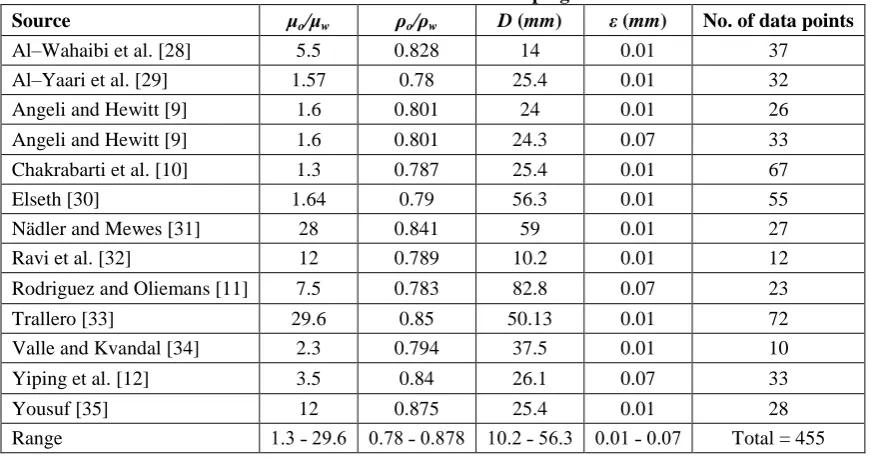
Tabel 1. Details of data bank used for developing the ANN model.

Source μo/μw ρo/ρw D (mm) ε (mm) No. of data points

Figure 1. Schematic representation of the developed single hidden layer ANN model.

Therefore, a single hidden layer network was used to obtain an accurate prediction in this study. For output layer neurons a linear transfer function were used, while for hidden layer neurons a tansig transfer function was applied. The network were designed and trained using 455 experimental data points collected from 13 sources of experimental data available in the literature which their details are presented in Table 1.

Superficial velocity of water (usw) and oil

(uso), viscosity ratio (μo/μw) and density ratio (ρo/ρw) of oil to water, inner diameter (D) and roughness of pipe (ε) were chosen as input variables of the network, while corresponding pressure gradient was selected as its target. Topology of the proposed network is shown in Figure 1.

As the raw input data must be preprocessed to convert them into a suitable form [39], all data were scaled to a similar magnitude in the range of [–1,1]. The input database were randomly divided into three sets: 65% (296 data points), 15% (68 data points) and 20% (91 data points) of the data points were used as training, validation and testing data sets, respectively. The training

data set was used to develop and adjust the weights and the biases in the network, the validation data set was used to ensure the accuracy and the generalization of the developed network during the training process, and the testing data set was used to examine the final performance of the network.

The total number of neurons in the input and output layers is equal to the number of input and output variables, respectively, while the optimal number of neurons in the hidden layer is normally not known at the start of the neural network training and depends on the complexity of the problem. Thus, it is estimated by trial–and–error method. The optimal number of neurons in the hidden layer was estimated through minimizing mean squared error (MSE) of testing data set defined as:





1

1 MSE

n

Exp i Pred i i

Y Y

n 





Where n is the number of data points, YPred

is the predicted value obtained from the neural network model and YExp is the

experimental value. The best performance

.

.

.

Pressure Gradient Output

Layer Hidden

Layer

μo/μw

D uso

usw

ρo/ρw Input Layer

wj,k

w1,j

ε

bj

of this single hidden layer MLP network was obtained with 16 neurons in the hidden layer. The performance of the developed optimal network model was evaluated by calculating coefficient of determination (R2) and average absolute percent (AAPE) error defined as:









2

, ,

2 1

2

, ,

1

R 1

n

Exp i Pred i i

n

Exp i Exp i i

Y Y

Y Y





  







, ,

1 ,

-1

AAPE 100

n

Exp i Pred i

i Exp i

Y Y

n  Y

 

 

 





Where Y_Expin Eq. 2 is the average of the experimental values. The results of the developed optimal network on training, validation and testing data are represented in Figures 2 and 3 and Table 2.

Figure2: Scatter plot of the ANN model predicted versus experimental values for training data set.

3: Scatter plots of the ANN model predicted versus experimental values for validation and testing data sets.

0 500 1000 1500 2000 2500 3000

0 500 1000 1500 2000 2500 3000

P

red

icted

p

ress

u

re

g

rad

ien

t

(P

a/m

)

Experimental pressure gradient (Pa/m)

0 200 400 600 800 1000 1200 1400 1600 1800 2000

0 500 1000 1500 2000

P

red

icted

p

ress

u

re

g

rad

ien

t

(P

a/m

)

Experimental pressure gradient (Pa/m)

Testing data set

Table2. Performance comparison of the ANN model for training, validation and testing data.

Data set R2 AAPE (%)

Training 0.998 7.12 Validation 0.986 9.37 Test 0.994 7.57

As can be seen from them, the developed network has very good prediction for all data sets.

2.2. Comparison of the ANN model and Al–Wahaibi correlation results

Al–Wahaibi [13] developed a pressure gradient correlation for horizontal oil–water separated flow by fitting the Fanning friction factor to Angeli and Hewitt [9] pressure gradient data for both acrylic and steel pipes and modified the friction factor proposed by Zigrang and Sylvester [40] for single phase flow. The Al–Wahaibi pressure gradient correlation [13] was proposed as follows:

0.8 2

2.4 2

cor m m

f u dp dx D     _{ }

  (4)

Where 2.4 is a dimensional coefficient

fitting parameter in

0.2 2 2       kg

m s , um is the mixture velocity in m/s, D is the pipe diameter in m and _m is the mixture density in kg/m3 given as:

_m H_w_w H_o_o

(5)

Where _w and _o are water and oil density, respectively, and Hw and Ho are

water and oil holdup, respectively, given by:

 w w w o Q H Q Q (6)

Where Qw and Qo are volumetric flow rates of water and oil, respectively. Likewise, fcor

presented in Eq. 4 is friction factor for two– phase oil–water flow given as:

1.11

1 4.518 6.9

2

0.25 _{m m} 0.25

cor D D log log Re Re f     _{ }      _  _ _{ } _       (7)

Where  is the wall roughness (1 10 5m

for the acrylic pipe and 7 10 5 m for the steel pipe) and Rem is mixture Reynolds number defined as:

m m m m u D Re  

 (8)

Where _m was proposed average mixture viscosity similar to Dukler et al. [41] average viscosity correlation:

_m H_w_w H_o_o

(9)

Where _w and _o are the water and oil viscosity, respectively.

The accuracy of predicted results from Al–Wahaibi correlation was compared to ANN model results for all data points (see Figures 4 and 5 and Table 3).

reported in Table 4 to allow other investigators to reproduce the results and make appropriate use of the ANN model, in which k is the number of input variables, j is the neuron number in the hidden layer and i

is the number of the output variables.

3. Sensitivity analysis

A sensitivity analysis was carried out to identify the degree of importance of input variables on the model outputs based on the

weight magnitude of the trained network. For this purpose, Garson equation [42] was applied as follows:

   

   

16 6

( , )

, ,

1 1

6 16 6

( , )

, ,

1 1 1

 

  

 _ 

  

 

 



  _ 

   

 _{  }

 





 



i j

m j k j

j k

m

i j

k j k j

k j k

IW IW LW

I

IW IW LW

(10)

Table3. Comparison of the accuracy of the developed ANN model and the Al–Wahaibi correlation against experimental database obtained from different sources.

Source AAPE (%)

Proposed ANN model Al–Wahaibi correlation

Al–Wahaibi et al. [28] 3.4 20.88 Al–Yaari et al. [29] 4.67 10.9 Angeli and Hewitt [9] acrylic 4.69 16.71 Angeli and Hewitt [9] steel 3.7 6.86 Chakrabarti et al. [10] 10.82 20.29 Elseth [30] 3.32 5.86 Nädler and Mewes [31] 5.68 16.88 Ravi et al. [32] 8.87 89.87 Rodriguez and Oliemans [11] 14.52 15.09 Trallero [33] 8.61 24.37 Valle and Kvandal [34] 4.04 2.6 Yiping et al. [12] 8.03 10.68 Yousuf [35] 4.74 10.33 All experimental data points 7.54 17.17

Figure4. Scatter plot of the ANN model predicted versus experimental values for all data

0 500 1000 1500 2000 2500 3000

0 500 1000 1500 2000 2500 3000

P

red

icted

p

ress

u

re

g

rad

ien

t

(P

a/m

)

Experimental pressure gradient (Pa/m)

Figure5. Scatter plot of the Al–Wahaibi correlation predicted versus experimental values for all data.

Table4. Weights and biases of the optimal ANN topology.

Neuron Hidden layer Output layer

Weights (j,k) Biases (j) Weights (i,j) Bias(i)

j wj,1 wj,2 wj,3 wj,4 wj,5 wj,6 bj w1,j b1

1 0.100756 –1.07841 1.002267 –2.64697 –1.50143 0.885123 –3.95651 –0.62978 0.938946

2 –2.37284 –1.25205 1.227268 –0.73326 4.567173 –1.20966 1.124103 0.641389

3 0.940672 –3.26921 –0.17716 3.922392 –0.21616 –1.68233 –2.20592 1.599259

4 –3.12513 –1.61818 –5.86737 –0.64546 –1.00819 1.443973 0.571192 –0.34633

5 0.940099 0.460423 3.895193 1.52139 –1.16866 –1.67258 –4.47733 –2.65837

6 4.130977 0.973065 2.415612 –0.98918 –1.96657 2.925324 –1.21452 0.964506

7 0.533085 –1.42444 2.325002 –0.03876 –2.11424 –1.92917 –4.15096 0.475042

8 0.806095 0.587852 –1.39918 –0.23092 –0.76923 0.217276 –1.27264 3.464686

9 3.922877 1.050652 –2.95362 1.981989 2.077173 –0.87049 0.641505 0.290049

10 –2.26633 –1.36202 3.5711 0.304896 2.254906 0.18226 1.034913 0.242732

11 –0.77642 2.978848 1.443499 –3.4489 –0.0282 1.979905 3.516165 1.839387

12 –0.56674 3.157595 1.623307 –1.43994 4.163803 1.37621 2.805941 0.178576

13 2.439082 1.076698 –1.86869 –1.61801 0.462946 0.85186 5.205034 –0.39629

14 –3.31565 –1.96467 2.527963 2.495823 5.410379 2.56447 –2.89956 –0.35702

15 0.488302 1.4565 –1.21186 –1.04279 0.241925 0.356546 4.848856 –0.57041

16 –3.09124 3.360507 0.937642 –0.72155 –5.60284 –1.44391 –1.86815 –0.27157

0 500 1000 1500 2000 2500 3000

0 500 1000 1500 2000 2500 3000

P

re

d

ic

te

d

p

re

ssu

re

g

ad

ie

n

t

(P

a/

m)

Experimental pressure gradient (Pa/m) R2_{= 0.884}

Where Im is the relative importance of the mth input variable on the output variable,

IW is the connection weights between the input neurons k and the hidden neurons 𝑗, and LW is the connection weights between the hidden neurons 𝑗 and the output neuron

i, respectively. Table 5 shows the relative importance (%) of each input variable on the ANN output.

Table5. Results of the sensitivity analysis for evaluating the effectiveness of the input variables

on the ANN output.

Input variables

Relative importance (%)

usw

14.96

uso

16.37

D 24.43

μo/μw

16.92

ρo/ρw

14.20

ε 13.12

As can be seen from Table 4, the pipe diameter (D) is the most important input variable (24.43%) of the ANN model, while other parameter have nearly the same important and there is no significant difference between the degree of importance of them. However, apart from

the mentioned variables, the pressure gradient can be affected by other parameters such as wettability characteristics of pipe materials [9], interfacial tension of the oil– water [35] and sub–flow regimes.

4. Conclusion

By using a total of 455 data points collected from 13 data sources, a neural network model was developed to predict the pressure gradient in horizontal liquid–liquid separated flow, regardless of its sub–flow regimes. The superficial velocities of oil and water, viscosity ratio and density ratio of oil to water, roughness and inner diameter of pipe were adopted as input parameters of the multilayer perceptron neural network (MLP–NN). The pressure gradient with a good accuracy (R2=0.996& AAPE=7.54%) was estimated using the optimal topology of the ANN. In addition, the accuracy of the developed ANN model was compared to Al–Wahaibi correlation and the results demonstrated that the proposed neural network model has better performance than Al–Wahaibi correlation having R2=0.884 and AAPE=17.17%. Finally, a sensitivity analysis carried out on the optimal trained ANN revealed that the pipe diameter has the most relative importance (24.43%) on the ANN output.

References

1- Xu, X. (2007). “Study on oil–water two–phase flow in horizontal pipelines.” J. Pet. Sci.Eng., Vol. 59, pp. 43–58.

2- Bannwart, A.C., Rodriguez, O.M.H., de Carvalho, C.H.M., Wang, I.S., Vara, R.M.O. (2004). “Flow patterns in heavy crude oil–water flow.” J. Energy. Res. Technol. Trans., Vol. 126, No. 3, pp. 184–189. 3- Charles, M.E., Govier, G.W., Hodgson, G.W. (1961). “The horizontal pipeline flow of equal density oil–

water mixtures.” Can. J. Chem. Eng., pp. 27–36.

4- Mandal, T.K., Chakrabarti, D.P., Das, G. (2007). “Oil water flow through different diameter pipes– similarities and differences.” Trans. IchemE. Part A. Chem. Eng. Res. Des., Vol. 85, No. A8, pp. 1123– 1128.

5- Wegmann, A., von Rohr, P.R. (2006). “Brief communication: two phase liquid–liquid flows in pipes of small diameters.” Int. J. Multiphase Flow, Vol. 32, pp. 1017–1028.

7- Charles, M.E., Lilleleht, L.U. (1966). “Correlation of pressure gradients for the stratified laminar–turbulent pipeline flow of two immiscible liquids.” Can. J. Chem. Eng., Vol. 44, pp. 47–49.

8- Stapelberg, H.H., Mewes, D. (1994). “The pressure loss and slug frequency of liquid–liquid–gas slug flow in horizontal pipes.” Int. J. Multiphase Flow, Vol. 20, pp. 285–303.

9- Angeli, P., Hewitt, G.F. (1998). “Pressure gradient in horizontal liquid–liquid flows.” Int. J. Multiphase Flow, Vol. 24, No. 7, pp. 1183–1203.

10- Chakrabarti, D.P., Das, G., Ray, S. (2005). “Pressure drop in liquid–liquid two phase horizontal flow: experiments and prediction.” Chem. Eng. Technol., Vol. 28, pp. 1003–1009.

11- Rodriguez, O.M.H., Oliemans, R.V.A. (2006). “Experimental study on oil–water flow in horizontal and slightly inclined pipes.” Int. J. Multiphase Flow, Vol. 32, pp. 323–343.

12- Yiping, L., Hua, Z., Shuhua, W., Jing, W. (2008). “Prediction of pressure gradient and holdup in small Eötvös number liquid–liquid segregated flow.” Chinese J. Chem. Eng., Vol. 16, No. 2, pp. 184–191. 13- Al–Wahaibi, T. (2012). “Pressure gradient correlation for oil–water separated flow in horizontal pipes, Exp.

Therm. Fluid Sci., Vol. 42, pp. 196–203.

14- Zhang, G., Patuwo, B.E., Hu, M.Y. (2002). “Forecasting with artificial neural networks: to optimum bit selection.” Comput. Geosci., Vol. 28, pp. 131–141.

15- Sablani, S.S., Shayyab, W.H., Kacimovc, A. (2003). “Explicit calculation of the friction factor in pipeline flow of Bingham plastic fluids: a neural network approach.” Chem. Eng. Sci., Vol. 58, pp. 99–106.

16- Goutorbe, B., Lucazeau, F., Bonneville, A. (2006). “Using neural networks to predict thermal conductivity from geophysical well logs, Artificial neural network for the evaluation of CO2 corrosion in a pipeline

steel.” Geophys. J. Int., Vol. 166, pp. 115–125.

17- Bassam, A., Ortega–Toledo, D., Hernández, J.A., González–Rodriguez, J.G., Uruchurtu, J. (2009). “Artificial neural network for the evaluation of CO2 corrosion in a pipeline steel.” J. Solid State Electr.,

Vol. 13, pp. 773–780.

18- Osman, E.A., Aggour, M.A. (2002). “Artificial Neural Network Model for Accurate Prediction of Pressure Drop in Horizontal and Near–Horizontal–Multiphase Flow.” Pet. Sci. Technol., Vol. 20, No. 1–2, pp. 1–15. 19- Osman, E.A. (2001). “Artificial Neural Networks Models for Identifying Flow Regimes and Predicting Liquid Holdup in Horizontal Multiphase Flow.” SPE Middle East Oil and Gas Show and Conf., Bahrain, 68219.

20- Shippen, M.E., Scott, S.L. (2002). “A Neural Network Model for Prediction of Liquid Holdup in Two– Phase Horizontal Flow.” SPE J., 77499.

21- Malayeri, M.R., Steinhagen, H.M., Smith, J.M. (2003). “Neural network analysis of void fraction in air/water two–phase flows at elevated temperatures.” Chem. Eng. Process, Vol. 42, pp. 587–597.

22- del Castillo, A.Á., Santoyo, E., García–Valladares, O. (2012). “A new void fraction correlation inferred from artificial neural networks for modeling two–phase flows in geothermal wells.” Comput. Geosci., Vol. 41, pp. 25–39.

24- Al–Naser, M., Elshafei, M. (2015). “Two–phase flow regimes identification using artificial neural network with nonlinear normalization.” proceedings of the 2nd international conference on fluid flow, Heat and Mass Transfer Ottawa, Ontario, Canada.

25- Shirley, R., Chakrabarti, D.P., Das, G. (2012). “Artificial neural networks in liquid–liquid two–phase flow.” Chem. Eng . Commun., Vol. 199, pp. 1520–1542.

26- Raj, T.S., Chakrabarti, D.P., Das, G. (2005). “Liquid–liquid stratified flow through horizontal conduit.”

Chem. Eng. Technol., Vol. 28, pp. 899–907.

27- Dasari, A., Desamala, A.B., Dasmahapatra, A.K., Mandal, T.K. (2013). “Experimental studies and probabilistic neural network prediction on flow pattern of viscous oil–water flow through a circular horizontal pipe.” Ind. Eng. Chem. Res., Vol. 52, No. 23, pp. 7975–7985.

28- Al–Wahaibi, T. Smith, M., Angeli, P. (2007). “Effect of drag–reducing polymers on horizontal oil–water flows.” J. Pet. Sci. Eng., Vol. 57, No. 3–4, pp. 334–346.

29- Al–Yaari, M., Soleimani, M.A., Abu–Sharkh, B., Al–mubaiyedh, U., Al–sarkhi, A. (2009). “Effect of drag reducing polymers on oil–water flow in a horizontal pipe.” Int. J. Multiphase Flow, Vol. 35, pp. 516–524. 30- Elseth, G. (2001). “An experimental study of oil–water flow in horizontal pipes, PhD. Thesis, The

Norwegian University of Science and Technology, Porsgrunn.

31- Nädler, M., Mewes, D. (1997). “Flow induced emulsification in the flow of two immiscible liquids in horizontal pipes.” Int. J. Multiphase Flow, Vol. 23, pp. 55–68.

32- Ravi, P., Sharma, M. Gosh, Das, G., Das, G.P.K. (2010). “Effects of return bands on kerosene– water flow through a horizontal pipe.” 7th Int. Conf. on Multiphase Flow, ICMF 2010, Tampa, Florida. USA.

33- Trallero, J.L. (1995). “Oil–water flow patterns in horizontal pipes.” PhD. Thesis, University of Tulsa. USA. 34- Valle, A., Kvandal, H. (1995). “Pressure drop and dispersion characteristics of separated oil/water flow.”

Two Phase Flow Model Exp., pp. 583–592.

35- Yousuf, N. (2011). “Experimental study in horizontal oil–water flow.” PhD. Thesis, Ahmadu Bello University, Nigeria.

36- Razavi, M.A., Mortazavi, A., Mousavi, M. (2003). “Dynamic modeling of milk ultrafiltration by artificial neural network.” J. Membrane Sci., Vol. 220, pp. 47–58.

37- Saini, L.M., Soni, M.K. (2002). “Artificial neural network based peak load forecasting using Levenberg– Marquardt and quasi–Newton methods.” IEE Proceedings of Generation, Trans. Distrib., Vol. 149, pp. 578–584.

38- Hush, D., Horne, B.G. (1993). “Progress in supervised neural networks.” IEEE Signal Proc. Mag., Vol. 10, pp. 8–39.

39- Karimi, H., Yousefi, F., Rahimi, M.R. (2011). “Correlation of viscosity in nanofluids using genetic algorithm–neural network (GA–NN).” Heat Mass Transfer, Vol. 47, pp. 1417–1425.

40- Zigrang, D.J., Sylvester, N.D. (1985). “A review of explicit friction factor equations.” J. Energ. Res. Technol., Vol. 107, pp. 280–283.

41- Dukler, A.E., Wicks, M., Cleveland, R.G. (1964). “Pressure drop and hold–up in two–phase flow.” AIChE. J., Vol. 10, pp. 38–51.