On Fuzzy Multi-Objective Multi-Item
Solid Transportation Problems
E. E. Ammar
1, and H. A. Khalifa
21- Department of Mathematics, Faculty of Science, Tanta University, Tanta, Egypt.
2- Department of Operations Research, Institute of Statistical Studies and Research, Cairo University, Cairo, Egypt.
Abstract
In general. There is no single optimal solution in multi-objective problems, but rather a set of non inferior (pareto optimal) solutions from which the decision maker (DM) must select the most preferred or best compromise solution as the one to implement. In this paper, a objective multi-item solid transportation problem by incorporating fuzzy numbers into the coefficients of the objective functions
(
c
i j kr p)
and / or supply quantities(
a
ip)
and / or demand quantities(
b
jp)
and / or conveyance capacities(
e
k)
. The concept of
-fuzzy efficient solution is introduced in which the ordinary efficient solution is extended based on the
-levels of fuzzy numbers. A necessary and sufficient condition for such a solution is established. The existing results concerning the qualitative analysis of the notions (solvability set and stability set of the first kind under the concept of
-parametric optimality are studied. A solution procedure for determining the stability set of the first kind corresponding to one of
-pareto optimal solution is proposed. An illustrative numerical example is given to clarify the obtained results.Keywords: Multi-objective multi-item solid transportation; fuzzy numbers;
-fuzzy efficient;
-optimality; parametric analysis.1. Introduction
The solid transportation problem (STP) is an extension of the classical transportation problem (TP) in which three item properties (supply, demand and conveyance) are taken into account in the constraint set instead of two items (supply and demand). The STP was first stated by Shell (1955) . A variety of approaches have been developed by many authors for multi-objective transportation problem (MOTP), Hussein (1998), and Das et al. (1999)). Some of the most important work related to STP are as follows:
Gen et al. (1995) proposed genetic algorithm for solving bicriteria STP with fuzzy numbers. Ojha et al. (2010) studied TP model with fixed charges and vechile costs where all unit discount (AUD). Incremental quantity discount (IQD) or combination of AUD and IQD on the price depending upon the amount is offered and varies on the choice of origin, destination and conveyance. Himenez and Verdegay (1999) introduced fuzzy STP in the case in which the fuzziness affects the constraint set. Ida et al. (1995) considered multi-criteria STP with fuzzy numbers; Li et al. (1997) presented a genetic algorithm for solving multi-objective STP with coefficient of the objective function as fuzzy numbers. Yang and Yuan (2007) investigated a bicriteria STP under stochastic environment. Bit et al. (1993) applied fuzzy programming approach to solve multi-objective STP. Nagarjan and Jeyaramon (2010) studied multi-objective STP with parameters as stochastic intervals. Kundu et al. (2013) introduced multi-objective multi-item STP with fuzzy coefficient for the objectives and constraints. Ammar and Khalifa (2014) studied multiobjective solid transportation problem with fuzzy numbers. Ammar and Khalifa (2015) studied multiobjective solid transportation problem with possibilistic variables.
Qualitative analysis of some basic notions such as the set of feasible parameters, solvability set, stability set of the first kind and stability set 0of the second and were introduced by Osman (1977). Sakawa and Yano (1989) introduced the concept of
-parametric optimality in fuzzy parametric programs.In this paper, a multi-objective multi-item solid transportation problem (FMOMISTP) with fuzzy numbers in the objective functions coefficients, supply values, demand values and conveyance is studied. The concepts of fuzzy efficient and
-parametric efficient solutions are introduced. Therelation between such solutions is given. A parametric analysis is used to characterize the set of all
-parametric efficient solutions. A solution procedure to determine the stability set of the first kind corresponding to one parametric efficient solution of FMOMISTP problem is presented. An illustrative numerical example is given in the sake of the paper to clarify the obtained results.2. Preliminaries
Here, some definition needed through this paper are recalled.
Definition 1: (Dubois and Prade (1980)). A fuzzy number
( )
q
is convex normalized fuzzy set of the real line R such that:(a)
x
0
R
,
q(
x
0)
1(
x
0 is called the mean value ofq
); (b)
q is piecewise continuous.Definition 2: (Dubois and Prade (1980)). The
-level set of the fuzzy numberq
is defined as theordinary set
L
( )
q
for which the degree of their membership functions exceed the level
:( )
q
{ :
q
q( )
q
,
[ 0, 1]}
.Throughout this paper,
F R
(
)
denoted the set of all compact (i.e., bounded and closed) fuzzynumbers on R, that is, for an
f
F R
(
)
of satisfies: (i) There exists
R
such thatf
(
x
)
1
;(ii) For any
( 0, 1], (
f
)
[
f
L,
f
U]
is closed interval on R.Observe that
R
F R
(
)
.The following notations are used in FMOMISTP:
c
i j kr p,
a
ip,
b
jp and(
),
k
e
F R
r
1, ..., ;
s
p
1, ...,
t
;i
1, ...,
m
;
j
1, ..., ;
n k
1, ...,
, and their
-level sets are:( )
(
)
( )
{
:
r p(
)
,
1, ..., ;
1, ..., ;
i j k
r p s t m n r p
i j k c i j k
c
c
c
R
c
r
s
p
t
1, ...,
;
1, ...,
;
1, ..., }
i
m
j
n k
,(
)
( )
{
:
p(
)
,
1, ..., ;
1, ...,
}
i
p t m p
i a i
a
a
a
R
a
p
t i
m
,(
)
( )
{
:
p(
)
,
1, ..., ;
1, ...,
}
j
p t n p
j b j
b
b
b
R
b
p
t
j
n
,(
)
( )
{
:
(
)
,
1, ..., }
k
k e k
e
e
e
R
e
k
,3. Problem formulation
A multi-objective multi-item solid transportation problem with fuzzy parameters
(FMOMSTP) is
(FMOMSTP)
1 1 1 1
min
( ,
)
,
t m n
r p p r
r i j k i j k
p i p k
z
x c
c
x
r
1, ...,
s
subject to
1 1
( , , ) {
:
,
1, ..., ;
1, ...,
n
p p
t m n
i j k i j k
M a b e
x
R
x
a
p
t i
m
;1 1
,
1, ..., ;
1, ...,
m
p p
i j k j
i k
x
b
p
t
j
n
;1 1 1
,
1, ...,
t m n
p k i j k
p i j
x
e
k
;1 1
,
1, ...,
m n
p p
i j
i j
a
b
p
t
,1 1 1
t n
p
k j
k p j
e
b
,0,
1, ..., ;
1, ...,
;
1, ..., ;
1, ..., }
p i j k
x
p
t
i
m
j
n k
where p
( 1, ..., )
t
items are to be transported from m origins to n distributions by means of k( 1, ..., )
different modes of transportation (conveyance). For the objectivez
r,
c
i j kr p represents fuzzy unit transportation penalty from ith origin to jth destination by kth conveyance for pth item.a
ip andp j
b
represent total fuzzy supply of ith origin and total fuzzy demand of jth destination, respectively forpth item. Also,
e
k is the total fuzzy capacity of kth conveyance. All ofc
i j kr p,
a
ip,
b
jp, ande
k areassumed to be characterized as trapezoidal fuzzy numbers, and
M a b e
( , ,
)
is compact set.Definition 3. (α-fuzzy Feasible actions): Let
1
(
11, ...,
1m)
ii
[ 0, 1]
,i
1, ...,
m
;2
(
21, ...,
2n),
2j[ 0, 1],
j
1, ...,
n
; and
3
(
31, ...,
3n)
,3k
[ 0, 1],
k
1, ..., ;
. Then}
,...,
1
;
,...,
1
;
,...,
1
;
,...,
1
,
0
:
{
x
R
* **x
p
t
i
m
j
n
k
l
M
x
tmnl ijkp
is said to be
-possible actions for problem (FMOMISTP) if :1 1
1
1 1
sup
(
p)
,
1, ...,
;
i n
p r i j k i
j k
n
p p
i j k i a i
j k
x a
x
a
i
m
1 1
2 1 1
sup
(
p)
,
1, ...,
;
j m
p r i j k j i k
m
p p
i j k j b j
i k
x b
x
b
j
n
1 1 1
3
1 1 1
sup
(
)
,
1, ..., ;
k
t m n
p k i j k
p i j
t m n
p
i j k k e k
p i j x e
x
e
k
where
denotes membership function.Definition 4. (α-fuzzy efficient): A point
x
*(
c
*)
M a
(
*,
b
*,
e
*)
is said to
-fuzzy efficientsolution to FMOMISTP problem if there is no
x c
(
*)
G a
(
*,
b
*,
e
*)
such that( ) 1 * *1 ( 1)
1 1 1
{
s t m n:
( ,
r)
(
,
), ...,
( ,
rc
c
R
z
x c
z
x
c
z
rx c
* ( 1) * * ( 1)
1
(
,
),
( ,
)
(
,
),
1( ,
)
r r r r
r r r r
z
x
c
z
x c
z
x
c
z
x c
(1)* ( 1) * * *
1
(
,
), ...
( ,
)
(
,
)}
,
r s s
r s s
z
x
c
z
x c
z
x
c
[ 0, 1]
where
denotes membership function. On account of the extension principle,( ) *1 * *1 ( 1)
1 1 1
{
s t m n:
( ,
)
(
,
), ...,
( ,
rc
c
R
z
x c
z
x
c
z
rx c
* ( 1) * * * ( 1)
1
(
,
),
( ,
)
(
,
),
1( ,
)
r r r r
r r r r
z
x
c
z
x c
z
x
c
z
x c
* ( 1) * * *
1
(
,
), ...,
( ,
)
(
,
)}
r s s
r s s
z
x
c
z
x c
z
x
c
1 1
1
( , ..., )
sup
min (
(
), ...,
s(
) )
s
s
c c
c c c
c
c
, (2)
where
1 ( ) *1 * *1 *( 1)
1 1 1
{ , ...,
s)
s t m n:
( ,
)
(
,
), ...,
r( ,
r)
c
c
c
R
z
x c
z
x
c
z
x c
* *( 1) * * *
1
(
,
), ...,
( ,
)
(
,
)}
r s s
r s s
z
x
c
z
x c
z
x
c
(3)and r p
(
1, ..., ;
1, ..., ;
1, ...,
;
1, ..., ;
1, ..., )
i j k
c
r
s p
t i
m j
n k
ares t
(
m n
)
any membership functions.
4. Characterizing α-fuzzy efficient solution for FMOMISTP problem
For characterizing the
- fuzzy efficient solution for FMOMISTP problem, let us considerthe following
-parametric multi-objective multi-item solid transportation problem (
-PMOMISTP)(
-PMOMISTP)1 1 1 1
min
( ,
)
,
1, ...,
p
t m n
p
r i j k
p i j k
z
x c
c
r
s
subject to
( , , ),
i j kr p(
i j kr p) ,
1, ..., ;
1, ..., ;
1, ...,
;
1, ...,
;
1, ..., ;
i(
ip) ,
1, ...,
;
1, ..., ;
j
n
k
a
a
i
m
p
t
(
p) ,
1, ..., ;
1, ..., ;
(
) ,
1, ..., ;
j j k k
b
b
j
n
p
s e
e
k
1 1
(
)
(
) ,
1, ..., ;
m n
p p
i j
i j
a
b
p
t
1 1 1
(
)
(
) ,
t n
p p
k j
k p j
e
b
and0,
1, ..., ;
1, ...,
;
1, ..., ;
1, ...,
p i j k
x
p
t
i
m
j
n k
,where
(
c
i j kr p) , (
a
ip) , (
b
jp)
, and(
e
k)
denote the
-cuts of the fuzzy variables,
,
r p p p
i j k i j
c
a
b
, ande
k , respectively. By the convexity assumption, r p(
)
i j k
r p i j k
c
c
,(
) ;
p(
), (
) ;
p(
), (
)
i j
r p p p p p
i j k a i i b j j
c
a
a
b
b
; and(
), (
) ,
1, ..., ;
k
e
e
ke
k r
s
1, ..., ;
1, ...,
;
1, ...,
;
1, ...,
p
t i
m
j
n
k
are real intervals that will denoted as:[ (
c
i j kr p( ) ) , (
Lc
i j kr p( ) ) ], [ (
Ua
ip( ) ) , (
La
ip( ) ) ], [ (
Ub
jp( ) ) , (
Lb
jp( ) ) ]
U and[ (
e
k( ) ) , (
Le
k( ) ) ]
U , respectively.Definition 5. (α-parametric efficient): A point
x
*(
c
*)
M a
(
*,
b
*,
e
*)
is said to be
-parametric efficient solution for
-PMOMISTP problem if there are nox
M a
(
*,
b
*,
e
*)
is said to be
-parametric efficient solution for
-PMOMISTP problem if there are no* * *
(
,
,
)
x
M a
b
e
,c
i j kr p
[ (
c
i j kr p(
) ) , (
Lc
i j kr p(
) ) ]
U ,[ (
(
) ) , (
(
) ) ],
[ (
(
) ) , (
(
) )
]
p p L p U p p L p U
i i i j j i
a
a
a
b
b
b
andk
e
[ (
e
k( ) ) , (
Le
k( ) ) ]
U such that:z
r( ,
x c
r)
z
r(
x
*,
c
r)
, for allr
1, ...,
s
and strict inequality holds for at least one r.
Theorem 1.
x
*
M a
(
*,
b
*,
e
*)
is
-fuzzy efficient solution for FMOMUSTP problem if and only ifx
*
M a
(
*,
b
*,
e
*)
isx
*
M a
(
*,
b
*,
e
*)
parametric efficient solution for
-PMOMISTP problem.Proof: (The proof will be in contra positive direction).
Necessity: Let
x
*(
c
*)
M a
(
*,
b
*,
e
*)
be
-fuzzy efficient solution for FMOMISTP problem andx
*(
c
*)
M a
(
*,
b
*,
e
*)
be not
-parametric efficient solution for
-PMOMISTP problem. Then there isx
1(
c
*)
M a
(
*,
b
*,
e
*)
for* * * * * *
(
) ,
(
) ,
(
)
1 *
(
,
r)
(
,
r),
1, ...,
r r
z
x
c
z
x
c
r
s
,with strict inequality holds for at least one. This leads to:
( ) *1 * *1 1 *( 1)
1 1 1
{
s t m n:
( ,
)
(
,
), ...,
(
,
r)
c
c
R
z
x c
z
x
c
z
rx
c
* *( 1) 1 * * * 1 *( 1)
1
(
,
),
(
,
)
(
,
),
1(
,
)
r r r r
r r r r
z
x
c
z
x
c
z
x
c
z
x
c
* *( 1) 1 * * *
1
(
,
), ...,
(
,
)
(
,
)}
r s s
r s s
z
x
c
z
x
c
z
x
c
.This contradicts the
-fuzzy efficient ofx
*(
c
*)
M a
(
*,
b
*,
e
*)
for FMOMISTP problem and the necessary part is established.Sufficiency: Let
x
*(
c
*)
M a
(
*,
b
*,
e
*)
be
-parametric efficient solution for
-PMOMISTP problem andx
*(
c
*)
M a
(
*,
b
*,
e
*)
be not
-fuzzy efficient solution for FMOMISTP problem. Then there isx
2(
c
*)
M a
(
*,
b
*,
e
*)
such that:( ) 2 *1 * *1 2 *( 1)
1 1 1
{
s t m n:
(
,
)
(
,
), ...,
(
,
r)
c
c
R
z
x
c
z
x
c
z
rx
c
* *( 1) 2 * * * 2 *( 1)
1
(
,
),
(
,
)
(
,
),
1(
,
)
r r r r
r r r r
z
x
c
z
x
c
z
x
c
z
x
c
* *( 1) 2 * * *
1
(
,
), ...,
(
,
)
(
,
)}
r s s
r s s
z
x
c
z
x
c
z
x
c
,i.e.,
1 1
1
( , ..., )
sup
min (
(
), ...,
s(
) )
s
s
c c
c c c
c
c
, (4)
where
1 ( ) 2 *1 * *1 2 *( 1)
1 1 1
{( , ...,
s)
s t m n:
(
,
)
(
,
), ...,
r(
,
r)
c
c
c
R
z
x
c
z
x
c
z
x
c
* * 2 * * * 2 *( 1)
1
(
,
),
(
,
)
(
,
), ...,
1(
,
)
r r r r
r r r r
z
x
c
z
x
c
z
x
c
z
x
c
2 * * *
1
(
,
)
(
,
)}
s s
r s
z
x
c
z
x
c
.For this supremum to exist, there is
(
d
1, ...,
d
s)
c
with 11
min (
(
), ...,
c
d
s(
)
s
c
d
,then
1 1
1
( , ..., )
sup
min (
(
), ...,
s(
) )
s
s
c c
d d c
d
d
.
This contradicts (4). Then there is
(
d
1, ...,
d
s)
c
satisfying1
1
min (
(
), ...,
s(
) )
s
c
d
cd
(5)This contradicts the efficient of
x
*
M a
(
*,
b
*,
e
*)
for
-PMOMISTP problem, and the sufficiency part is proved.5. Parametric analysis
For characterizing the set of all parametric efficient solutions for
-PMOMISTP problem,we use the parametric optimization (scalarization) problem (here the weighting method (Chanas et al.
STP
(
w
)
1
min
( ,
)
s
r
r r
r
w z
x c
subject to
( , , ),
i j kr p(
i j kr p)
x
M a b e
c
c
,(
) ,
(
) ,
(
)
p p p p
k k
i i j j
a
a
b
b
e
e
,1 1
(
)
(
)
m n
p p
i j
i j
a
b
,1 1 1
(
)
(
)
t n
p p
i j
k p j
e
b
,1
0,
1, ..., ,
1
s
r r
r
w
r
s
w
, and0,
1, ..., ;
1, ...,
;
1, ..., ;
1, ...,
p i j k
x
p
t i
m
j
n k
.Definition 6. (α-parametric optimal): The set of
-parametric optimal solutions of STP(
w
)
is defined as:* * * *
1 1
(
)
:
(
,
)
( ,
)
s s
t m n r r
r r r r
r r
E w
x
R
w z
x
c
w z
c
,
for each
x c
(
*)
M a
(
*,
b
*,
e
*),
c
*
( ) ,
c
a
*
( ) ,
a
* *
( ) ,
( )
b
b
e
e
, and1
0,
1, ..., ,
1
s
r r
r
w
r
s
w
.Remark 1. A point
x
*(
c
*)
is said to be
-parametric efficient solution of
-PMOMISTPproblem with corresponding
-parametric optimal parameters(
c
*,
a
*,
b
*,
e
*)
if there exists *0
w
such thatx
* is the unique
-parametric optimal solution of STP(
w
)
.Remark 2. A point
x
*(
c
*)
is said to be a proper
-parametric efficient solution of
-PMOMISTP problem if and only if there existsw
*
0
such thatx
*
E w
(
*)
.Definition 7. The solvability set of
-PMOMISTP problem is denoted by B and is defined by:{
s:
B
w
R
there exists
-parametric efficient solutionx
* of
-PMOMISTP problem,
x
*
E w
(
)}
.{
,
0}
B
w
B w
.Remark 3. If
B
B
andx
*
E w
(
*),
w
*
B
, thenx
* is called a proper
-parametric efficient solution of
-PMOMISTP problem.Definition 9. Suppose that
x
*
B
with a corresponding
-parametric optimal solution* *
(
)
x
E w
, then the stability set of the first kind of
-PMOMISTP problem corresponding to*
x
, denoted asS x
(
*)
and is defined by:* * *
(
)
{
:
(
)
S x
w
B
x
E w
is an
-parametric optimal solution ofSTP
(
w
)
problem }.For determining the stability set of the first kind, let STP
(
w
)
reformulated as in the following form:(STP
(
w
) )
1
min
( ,
)
s
r
r r
r
w z
x c
subject to
1 1
( ,
)
,
1, ..., ;
1, ...,
;
n
p p p
i i i j k i
j k
f
x a
x
a
p
t i
m
1 1
( ,
)
,
1, ..., ;
1, ...,
;
m
p p p
i j i j k j
i k
g
x b
x
b
p
t
j
n
1 1
( ,
)
,
1, ..., ;
1, ...,
;
m n
p
k k i j k k
i j
h
x e
x
e
p
t
k
(
)
,
1, ..., ;
1, ..., ;
1, ...,
;
r p i j k
r p i j k
c
c
r
s
p
t
i
m
1, ..., ;
1, ..., ;
j
n k
(
)
,
1, ..., ;
1, ...,
;
p i
p i
a
a
p
t
i
m
(
)
,
1, ..., ;
1, ..., ;
p j
p j
b
b
p
t
j
n
(
)
,
1, ..., ;
k
e
e
kk
1 1
(
)
(
) ,
1, ...,
m n
p p
i j
i j
a
b
p
t
;1 1 1
(
)
(
) ;
r n
p
k j
k p j
e
b
1
0,
1, ..., ;
1
s
r r
r
w
r
s
w
0,
1, ..., ;
1, ...,
;
1, ...,
;
1, ...,
p i j k
x
p
t
i
m
j
n
k
and
[ 0, 1]
.Let
w
*
B
withx
* is
-parametric efficient solution for
-PMOMISTP problem, then the Kuhn-Tucker necessary optimality conditions corresponding to (STP(
w
) )
take the form:1 1 1 1
0,
1, ...,
;
s m n
r i i k
r i j k
r i j k
z
f
g
h
w
t
m n
x
x
x
x
1 1(
)
0,
1, ..., ;
1, ..., ;
1, ...,
;
i j k
r p r p
s s c i j k
r
r r p r r p
r i j k r i j k
c
z
w
u
r
s
p
t
i
m
c
c
1, ...,
;
1, ..., ;
j
m k
1 1
(
)
0,
1, ..., ;
p i
p
m m i
a i
i p i p
i i i i
a
f
p
t
a
a
1 1(
)
0,
1, ..., ;
p i
p
m m i
a i
i p i p
i i i i
a
f
p
t
a
a
1 1(
)
0,
1, ..., ;
p j
p
n n b j
i
j p j p
j j j j
b
g
p
t
b
b
1 1(
)
0,
k e k k k kk k k k
e
h
e
e
1 1( ,
)
,
1, ..., ;
1, ...,
n
p p p
i i i j k i
j k
f
x a
x
a
p
t i
m
; 1 1( ,
)
,
1, ..., ;
1, ...,
m
p p p
j j i j k j
i k
g
x b
x
b
p
t
j
n
; 1 1( ,
)
,
1, ..., ;
1, ...,
m n
p
u k i j k k
i j
h
x e
x
e
p
t
k
;(
)
,
1, ..., ;
1, ...,
r p i j k
r p i j k
c
c
r
s p
t
;(
)
,
1, ..., ;
1, ..., ;
1, ...,
;
r p i j k
r p i j k
c
c
r
s
p
t i
m
1, ...,
;
1, ...,
j
m k
;(
)
,
1, ..., ;
1, ...,
p i
p i
a
a
p
t i
m
;(
)
,
1, ..., ;
1, ...,
p j
p j
b
b
p
t
j
n
k
e
(
e
k)
,
k
1, ...,
;1 1
(
)
(
) ,
1, ...,
m n
p p
i j
i j
a
b
p
t
;1 1 1
(
)
(
) ,
t n
p
k j
k p j
e
b
( ,
p)
0,
1, ..., ;
1, ...,
;
i
f
ix a
ip
t i
m
( ,
p)
0,
1, ..., ;
1, ...,
;
j
g
jx b
jp
t
j
n
( ,
)
0,
1, ..., ;
k
h
kx e
kk
(
r p(
)
)
0,
1, ..., ;
1, ..., ;
1, ...,
;
1, ..., ;
i j k
r p
r c i j k
U
c
r
s e
t i
m j
n
1, ...,
k
;(
p(
)
)
0,
1, ..., ;
1, ...,
i
p
i a
a
ip
t i
m
;(
p(
)
)
0,
1, ..., ;
1, ...,
j
p
j b
b
jp
t
j
n
;(
(
)
)
0,
1, ...,
k
k e
e
kk
;,
,
,
,
,
i j k
U
r i j
and
k
0
,1, ...,
;
1, ..., ;
1, ...,
i
m
j
n k
,where
i,
j,
k,
U
r,
i,
j and
k are the Lagrange multipliers and the above expressions are evaluated at(
x
*,
c
*,
a
*,
b
*,
e
*)
. The first four relations with the last one of the above system represent a pobytope T for which vertices can be determined using any algorithm based on thesimplex method. According to whether any of the variables
(
1, ...,
),
(
1, ...,
),
(
1, ..., )
i
i
m
jj
n
kk
,U
r(
r
1, ..., )
s
,
i,
j and
k arezero or positive, the stability set of the first kind of (STP
(
w
) )
is determined.6. Solution procedure
The steps of the proposed procedure to determine
S x
(
*)
can be summarized as in the following steps:Step 1: Ask the DM to specify the initial value of
( 0
1)
, say
*
0
).Step 2: Elicit a membership function for each of the fuzzy numbers
c
i j kr p,
a
ip,
b
jp, and,
1, ..., ;
1, ..., ;
1, ...,
,
1, ..., ;
1, ...,
k
e
r
s
p
t
i
m
j
n
k
in
Step 3: Construct the parametric nonlinear programming problem (STP
(
w
) )
.Step 4: Choose certain
w
*
B
and solve (STP(
w
) )
problem using any available computerpackage. Let
x
* be
-parametric optimal solution of (STP(
w
) )
with the corresponding
-level optimal parameters(
c
*,
a
*,
b
*,
e
*)
.Step 5: Substitute with
x
*,
c
*,
a
*,
b
* ande
* in the Kuhn-Tucker necessary optimality conditions and hence solve the resulted system.Step 6: Determine
S x
(
*)
according to the values of the Lagrange multipliers.Step 7: Set
1
(
*
)
( 0, 1]
0 and go to step 2.Repeat the above steps of the procedure until the interval
[ 0, 1]
is fully exhausted, they stop.7. Numerical example
Consider the FMOMISTP problem with
p
1, 2
i
,
j k r
,
,
. The unit transportation are given in the following tables:Table 1. Fuzzy unit transportation penalties / costs
c
11i j ki
j j
1 2 1 2
1 (6, 8, 9, 11) (4, 6, 9, 11) (9, 11, 13, 15) (6, 8, 10, 12)
2 (8, 10, 13, 15) (6, 7, 8, 9) (10, 12, 13, 15) (6, 8, 10, 12)
k 1 2
Table 2. Fuzzy unit transportation penalties / costs
c
12i j ki j j
1 2 1 2
1 (9, 10, 12, 13) (6, 8, 10, 12) (11, 13, 14, 16) (6, 7, 10, 11)
2 (11, 13, 14, 16) (7, 9, 12, 14) (14, 16, 18, 20) (9, 11, 12, 14)
k 1 2
Table 3. Fuzzy unit transportation penalties / costs
c
i j k21i j J
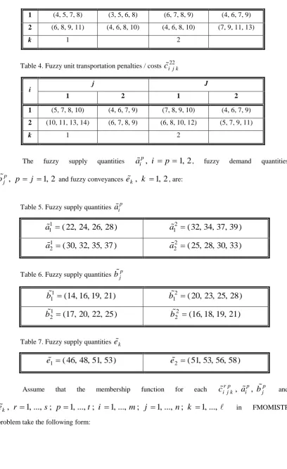
1 (4, 5, 7, 8) (3, 5, 6, 8) (6, 7, 8, 9) (4, 6, 7, 9)
2 (6, 8, 9, 11) (4, 6, 8, 10) (4, 6, 8, 10) (7, 9, 11, 13)
k 1 2
Table 4. Fuzzy unit transportation penalties / costs
c
i j k22i
j J
1 2 1 2
1 (5, 7, 8, 10) (4, 6, 7, 9) (7, 8, 9, 10) (4, 6, 7, 9)
2 (10, 11, 13, 14) (6, 7, 8, 9) (6, 8, 10, 12) (5, 7, 9, 11)
k 1 2
The fuzzy supply quantities
a
ip,
i
p
1, 2
, fuzzy demand quantities,
1, 2
p j
b
p
j
and fuzzy conveyancese
k,
k
1, 2
, are:Table 5. Fuzzy supply quantities
a
ip1
1
( 22, 24, 26, 28)
a
a
12
(32, 34, 37, 39)
1
2
(30, 32, 35, 37 )
a
a
22
( 25, 28, 30, 33)
Table 6. Fuzzy supply quantities
b
jp1
1
(14, 16, 19, 21)
b
b
12
( 20, 23, 25, 28)
1
2
(17, 20, 22, 25)
b
b
22
(16, 18, 19, 21)
Table 7. Fuzzy supply quantities
e
k1
( 46, 48, 51, 53)
e
e
2
(51, 53, 56, 58)
Assume that the membership function for each
c
i j kr p,
a
ip,
b
jp and,
1, ..., ;
1, ..., ;
1, ...,
;
1, ...,
;
1, ...,
k