The Immersed Boundary Projection Method and Its Application to Simulation and Control of Flows Around Low-Aspect-Ratio Wings

(1)

The immersed boundary projection method and its

application to simulation and control of flows around

low-aspect-ratio wings

Thesis by

Kunihiko Taira

In Partial Fulfillment of the Requirements for the Degree of

Doctor of Philosophy

California Institute of Technology Pasadena, California

2008

(2)

c

2008

(3)

iii

(4)

Acknowledgements

My advisor, Professor Tim Colonius, is gratefully acknowledged for his support and teachings throughout my graduate studies. His passion for research and sharp eyes for analyzing flow physics have been a great source of inspiration. I have truly enjoyed the moments discussing numerical methods and fluid mechanics with him on the whiteboard and by the round table in his office. Professors Morteza Gharib, Melany Hunt, and John Dabiri have offered enlightening comments and graciously agreed to serve on my committee.

I was also fortunate to be involved in a multi-disciplinary research initiative (MURI), receiving insightful comments by Professors Clarence Rowley (Princeton Univ), David Williams (Illinois Inst of Tech), Gilead Tadmor (Northeastern Univ), and Doctor William Dickson. Funding for this research was provided by the US Air Force Office of Scientific Research and some of the computations were made possible by the US Department of Defense High Performance Computing Modernization Program.

I must also thank Professor Jay Frankel (Univ of Tenn) for his guidance during both my undergraduate and graduate studies. He certainly has been a great influence on me for pursuing graduate studies. Appreciation also goes to Professor Raj Pal Soni (Univ of Tenn) for teaching me a series of unforgettable courses in Mathematics.

(5)

v

discussions with Eric Johnsen, Keita Ando, and Rick Burnes on fluid mechanics. Special thanks go to Jeff Krimmel and Jennifer Frank, who have been very kind and selfless in maintaining the computational resources. Won Tae Joe and Sunil Ahuja (Princeton Univ) are also thanked for patiently using my immersed boundary code and reporting bugs therein. Their inputs have been very valuable in improving the code.

Many of my other friends have made my life at Caltech enjoyable as well. Joseph Klamo and I sat together in many of the aeronautics courses (his note-taking skills were quite impressive). There were the three o’clock meetings with Mohamed El-Naggar and Kaushik Dayal that were just priceless. Tomonori Honda has helped me tremendously, particularly during my first year at Caltech, and has been a person I admire for his mathematical talent. Michael Wolf, Nicolas Hudson, Alexandros Taflanidis, and Chang Kook Oh have also been great friends. I cannot mention everyone here but I am thankful to all of those who have influenced me during my years at Caltech.

My parents, Kunio and Yasuyo Taira, have always supported and encouraged me in every choice I have made in life. I would not have been able to come this far without their constant support and care. Thank you. Appreciation also goes to my sister, Tomoko, for her support and occasional packages from Japan. With the completion of my graduate studies, I do hope I am able to make my father’s old dream come true.

(6)

Abstract

The immersed boundary projection method and its application to

simulation and control of flows around low-aspect-ratio wings

by

Kunihiko Taira

California Institute of Technology

(7)

vii

wake vortices are found to be the same across different aspect ratios and angles of attack. Behind low-aspect-ratio rectangular plates, leading-edge vortices form and eventually separate as hairpin vortices following the start-up. This phenomenon is found to be similar to dynamic stall observed behind pitching plates. The detached structure would then interact with the tip vortices, reducing the downward velocity induced by the tip vortices acting upon the leading-edge vortex. At large time, depending on the aspect ratio and angles of attack, the wakes reach one of the three states: (i) a steady state, (ii) a periodic unsteady state, or (iii) an aperiodic unsteady state. We have observed that the tip effects in three-dimensional flows can stabilize the flow and also exhibit nonlinear interaction with the shedding vortices.

(8)

List of Figures

2.1 Spatial discretization with a two-dimensional staggered grid. . . 11

2.2 Setup for the one-dimensional Stokes’ problem. . . 25

2.3 Error norms from the one-dimensional Stokes’ problem. . . 26

2.4 Setup for the problem of two concentric cylinders. . . 27

2.5 Error norms from the problem of two concentric cylinders. . . 28

2.6 Characteristic dimensions of the wake structure. . . 31

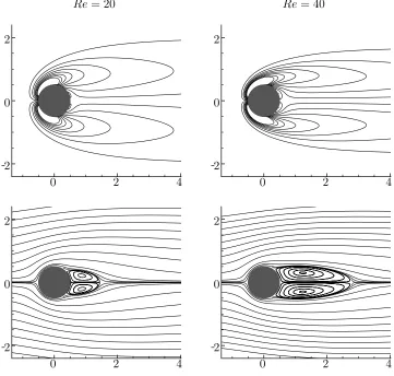
2.7 Vorticity field around a cylinder at Re= 20 and 40. . . 32

2.8 Vorticity field around a cylinder at Re= 200. . . 34

2.9 Vorticity field around a moving cylinder at Re= 40 and 200. . . . 36

2.10 Drag history of a cylinder forRe= 40 and 200. . . 37

2.11 Growth of the recirculation zone behind cylinders. . . 38

2.12 Steady-state vorticity field around a sphere at Re= 200. . . 39

3.1 A typical setup of the computational domain around the wing. . . 45

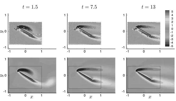
3.2 Comparison of the spanwise vorticity fields from the experiment and simulation. . . 46

3.3 Isosurface for the spanwise vorticity around the wing. . . 47

3.4 Lift and drag coefficients for a wing of AR= 2 at Re= 100. . . 48

3.5 Wake vortices behind rectangular plates of AR = 1, 2, and 4 at α = 30◦ andRe= 300. . . 50

(12)

3.8 Characteristic lift coefficients and lift-to-drag ratios for various rectangular plates. . . 58 3.9 Time at which lift achieves the maximum. . . 59 3.10 The POD mode, the weighted POD mode, and the lift-weighted

vortices of the wake. . . 62 3.11 Power spectra of the lift trace for a rectangular plate of AR= 3 at

Re= 500. . . 63 3.12 Stability of the wake for a range ofα and ARat Re= 300 and 500. 65 3.13 Top view of the asymmetric wake at large time behind a plate of

AR= 2. . . 66 3.14 Wake measurements and power spectra for a periodic case (I). . . . 68 3.15 Wake measurements and power spectra for an aperiodic case (II). . 68 3.16 Wake measurements and power spectra for an aperiodic case (III). 69 3.17 Wake vortices behind different planform geometries. . . 71 3.18 Time trace of lift and drag coefficients for various non-rectangular

planforms. . . 73 3.19 Convective transport of spanwise vorticity. . . 73

4.1 A schematic of the flow control setup. . . 80 4.2 Forces on the plate with leading-edge actuation for varied Cµ. . . . 81 4.3 Lift and drag on a rectangular wing ofAR= 2 with various actuations. 83 4.4 Modification of the wake structures from the use of midchord and

trailing-edge blowing in the downstream direction. . . 86 4.5 An illustration of tip vortices engulfing the trailing-edge vortex sheet

with trailing-edge actuation. . . 88 4.6 Time-averaged lift and lift-to-drag ratios for various aspect ratios

with and without actuation. . . 90 4.7 Normalized lift over normalized circulation of the tip vortex from

control. . . 91

(13)

xiii

5.2 Three-dimensional wake vortices around flapping plates. . . 96

B.1 Spatial discretization with a three-dimensional staggered grid. . . . 104 B.2 Schematic of 3-level multi-domain solution of the Poisson equation. 109 B.3 Potential flow over a circular cylinder computed by the fast

immersed boundary method with multi domains. . . 113 B.4 Velocity error from the multi-domain technique. . . 114 B.5 Vorticity field around an impulsively started cylinder forRe= 200. 117

C.1 Illustration of the two-dimensional windowing function. . . 121 C.2 Comparison of the the vorticity fields with the use of different

outflow boundary conditions. . . 122

(14)

List of Tables

2.1 Spatial and temporal simulation parameters for Re= 40 and 200. . 30 2.2 Results for steady flow around a cylinder at Re= 20 and 40. . . . 33 2.3 Results for unsteady flow around a cylinder at Re= 200. . . 35 2.4 Results for steady flow around a sphere at Re= 100 and 200. . . . 39

A.1 Nomenclature of the discrete operators and their continuous analogs. 99

B.1 Results for steady flow around a cylinder at Re= 40 computed by the fast immersed boundary method. . . 115 B.2 Results for unsteady flow around a cylinder atRe= 200 computed

(15)

1

Chapter 1

Introduction

1.1

Motivation and background

Traditionally most aerodynamic systems have been developed for steady operations. However, many biological systems have been observed to operate under unsteady conditions in low Reynolds number flows. For example, birds and insects use flapping motions to keep themselves aloft. Moreover, internal flows in cardiovascular systems are unsteady due to the periodic pumping of blood by the heart.

Analyzing such unsteady flows poses a great challenge to numerical simulations. In the majority of biological flows, the fluid evolves around or inside bodies of often complex geometries that are in motion and/or under deformation. Numerically speaking, spatial discretization (mesh generation) of these computational domains can become a problem by itself (Baker, 2005).

(16)

one that is fitted to the body. However, the need for re-gridding of the body-fitted mesh still exists for deforming bodies.

Here we explore methods that can be easily implemented into a widely available incompressible flow solver. In particular, we consider employing a simple Cartesian grid (Eularian) discretization over the entire domain including the immersed body and solving for the flow field using the well-known fractional step (projection) method to advance in time. Additionally, we let the body be discretized by a collection of surface points (Lagrangian), whose motion can either be prescribed or be based on some physics. At these Lagrangian points, regularized surface forces with appropriate magnitudes and directions are applied to enforce the no-slip boundary condition along the immersed surfaces.

With this approach, re-meshing is not required since only the location of the surface needs to be tracked. This method, the immersed boundary method, was originally introduced by Peskin (1972, 1977) to simulate the flows inside a heart. Based upon past immersed boundary methods (Peskin, 2002; Mittal & Iaccarino, 2005), here we present theimmersed boundary projection methodthat is stable and does not require any ad hoc constitutive relations for simulations of flows around bodies with known surface velocities.

Equipped with the immersed boundary projection method, we are able to simulate various external flows around animals and internal biological flows. Of particular interest in this thesis are the three-dimensional flows around low-aspect-ratio wings in pure translation. Such flows are fundamental for understanding flows around flapping bio-flyers (Shyyet al., 2008) as well as those over micro-air-vehicles (Mueller & DeLaurier, 2003). Here we focus on the unsteady nature of the separated flows and the corresponding forces generated by various low-aspect-ratio wings.

(17)

1.2 Outline of this thesis 3 results are to motivate future studies on applying feedback control upon the three-dimensional flows to enhance lift in some optimal fashion.

The applications considered here do not exhibit the full capability of the method. We note that the current simulation method can compute flows around entire animals such as insects and jellyfish as well as small-scale underwater vehicles. Furthermore, one can simulate internal flows with an immersed object such as the red blood cells within blood vessels. Fluid-structure interactions can also be considered with this method. The flexibility of this simulation methodology has been one of the main reasons for the pursuing the immersed boundary method. As this thesis is somewhat divided into the development of the numerical method and the analysis of the three-dimensional separated flows around the low-aspect-ratio wings, we have provided additional background information in each chapter to discuss further details on the subject in a more relevant manner.

1.2

Outline of this thesis

This thesis first introduces the immersed boundary projection method in Chapter 2. The derivation of this method is based upon the traditional fractional step/projection method used to solve for incompressible flows. Short discussions on the comparison of the current approach with previous methods are provided. Numerical examples are considered for the verification and validation of the method.

(18)

and compared with the unactuated cases.

At last in Chapter 5, we offer some concluding remarks and suggestions for future directions of research in both the immersed boundary projection method and low-Reynolds-number flows.

1.3

Resulting publications

Based on the work described in this thesis, the following archival papers have been written:

• Chapter 2

Taira, K. & Colonius, T. 2007 The immersed boundary method: a projection approach. J. Comput. Phys. 225, 2118–2137.

• Chapter 3

Taira, K. & Colonius, T. 2008 Three-dimensional separated flows around low-aspect-ratio flat plates. J. Fluid Mech. (submitted).

• Chapter 4

Taira, K. & Colonius, T. 2008 On the effect of tip vortices in low-Reynolds-number post-stall flow control. (to be submitted).

• Appendix B

(19)

5

Chapter 2

The Immersed Boundary

Projection Method

2.1

Introduction

Immersed boundary methods have gained popularity for their ability to handle moving or deforming bodies with complex surface geometry (Peskin, 2002; Mittal & Iaccarino, 2005). Peskin (1972) first introduced the method by describing the flow field with an Eulerian discretization and representing the immersed surface with a set of Lagrangian points. The Eulerian grid is not required to conform to the body geometry as the no-slip boundary condition is enforced at the Lagrangian points by adding appropriate boundary forces. The boundary forces that exist as singular functions along the surface in the continuous equations are described by discrete delta functions that smear (regularize) the forcing effect over the neighboring Eulerian cells.

(20)

control to compute the force on the rigid immersed surface. The difference between the velocity solution and the boundary velocity is used in a proportional-integral controller. For the aforementioned techniques to model flow over rigid bodies, the choice of gain (stiffness) remains ad hoc and large gain results in stiff equations. Our intention is to remove all tuning parameters and formulate the immersed boundary method in a general framework for rigid bodies (as well as bodies with prescribed surface motion).

(21)

2.2 Fractional step methods 7 the current formulation. Further details on the discretization of the immersed boundary projection method are placed in Appendix A.

2.2

Fractional step methods

We consider the incompressible Navier-Stokes equations

∂u

∂t +u· ∇u =−∇p+

1

Re∇

2_u_, _(2.1)

∇ ·u = 0, (2.2)

whereu,p, andReare the suitably non-dimensionalized velocity vector, pressure, and the Reynolds number, respectively. Following references (Chorin, 1968; T´emam, 1969; Kim & Moin, 1985; Perot, 1993; Changet al., 2002), the equations are discretized with a staggered-mesh finite volume formulation using the implicit Crank-Nicolson integration for the viscous terms and the explicit second-order Adams-Bashforth scheme for the convective terms. This produces an algebraic system of equations,

 A G

D 0    q n+1 p  =  r n 0  +  bc1

bc2



, (2.3)

where qn+1 and p are the discretized velocity flux and pressure vectors. The discrete velocity can be recovered by un+1 ₌ _R−1_qn+1_{, where} _R _{is a diagonal} matrix that transforms the discrete velocity into the velocity flux. Sub-matricesG

and D correspond to the discrete gradient and divergence operators, respectively. The operator resulting from the implicit velocity term is A = _∆t1 M − 1

2L, where

(22)

and in the works of Perot (1993) and Chang et al.(2002). It is interesting to note that G=₋DT _{for the staggered grid formulation.}

The traditional fractional step method by Chorin (1968) and T´emam (1969) was introduced to solve Eq. (2.3) in an efficient manner by using an approximation for A−1. In the present analysis, we adopt the observation made by Perot (1993) that the fractional step method can be regarded as an LU decomposition of Eq. (2.3):



 A 0

−GT GTBNG

 

 I B

N_G 0 I    q n+1 p   =  r n 0  +  bc1

bc2  +  − ∆tN

2N (LM−1)NGp

0



, (2.4) where BN is the N-th order Taylor series expansion ofA−1:

A−1∼=BN

= ∆tM−1+ ∆t 2

2 (M

−1_L₎_M−1₊_{· · ·}₊ ∆tN 2N−1(M

−1_L₎N−1_M−1

= N

X

j=1 ∆tj

2j−1(M

−1_L₎j−1_M−1_.

(2.5)

(23)

2.2 Fractional step methods 9 Equation (2.4) is more commonly written in three steps:

Aq∗=rn+bc1, (Solve for intermediate velocity) (2.6)

GTBNGp=GTq∗+bc2, (Solve the Poisson equation) (2.7)

qn+1=q∗−BNGp. (Projection step) (2.8)

Since bothAandGTBNGare symmetric positive-definite matrices, the conjugate gradient method can be utilized to solve the above momentum and Poisson equations in an efficient manner. In general, for non-symmetric matrices, various other Krylov solvers can be employed.

Here the discrete pressure is denoted by p without any superscript for its time level, as we regard pressure as a Lagrange multiplier (Chang et al., 2002). There has been extensive discussion on the exact time level of the discrete pressure variable for various treatments of pressure in fractional step methods (Strikwerda & Lee, 1999; Brownet al., 2001). For the present method,pis a first-order accurate approximation of pressure in time, vis. pn+1/2_{. Since the first-order accuracy of}

p does not affect the temporal accuracy of the velocity variable (Perot, 1993), we use p as a simple representation of the pressure variable. If a second-order accurate pressure is desired, Brown et al.(2001) should be referred to for further modifications to the fractional step method.

Although a detailed stability analysis is not offered in this paper, we demonstrate that the present method described in the next section can stably solve for the flow field for CFL numbers up to 1, as shown in Section 2.5. We mention that fractional step methods for incompressible flow can suffer numerical instability if ∆t is decreased arbitrarily (Guermond & Quartapelle, 1998). The time step is limited by a lower bound of ∆t_≥c∆xl+1_{if equal orders of interpolation} are used for velocity and pressure, as in the present case (c is a constant and l

(24)

We note in passing that the form of Eq. (2.3) is known as the Karush-Kuhn-Tucker (KKT) system that appears in constrained optimization problems (Nocedal & Wright, 1999). This system minimizes a term similar to the kinetic energy:

min qn+1

1 2(q

n+1₎T_Aqn+1₋₍_qn+1₎T₍_rn₊_bc 1)

subject to Dqn+1= 0 +bc2. (2.9)

It is interesting that the discrete pressure p does not play a direct role in time advancement, but acts as a set of Lagrange multipliers to minimize the system energy and satisfy the kinematic constraint of divergence-free velocity field.

2.3

The immersed boundary projection method

2.3.1

The discretized Navier-Stokes equations with

boundary force

Since the discretized Navier-Stokes equations, Eq. (2.3), are observed to be a KKT system with pressure acting as a set of Lagrange multipliers to satisfy the continuity constraint, one can imagine appending additional algebraic constraints by increasing the number of Lagrange multipliers. Hence we incorporate the no-slip constraint from the immersed boundary method into the fractional step framework. The immersed boundary method introduces a set of Lagrangian points, ξ_k, that represent the surface, ∂B, of an immersed object, B, within a computational domain,_D, whose geometry need not conform to the underlying spatial grid. At the Lagrangian points, appropriate surface forces,fk, are applied to enforce the no-slip condition along ∂_B. Figure 2.1 illustrates the setup of the spatial discretization. Since the location of the Lagrangian boundary points does not necessarily coincide with the underlying spatial discretization, two operators are required: one that passes information from the boundary points to the neighboring staggered grid points and another one that conveys information in the opposite direction.

(25)

2.3 The immersed boundary projection method 11

Figure 2.1: Staggered grid discretization of a two-dimensional computational

domain _D and immersed boundary formulation for a body _B depicted by a

shaded object. The horizontal and vertical arrows (→,↑) represent the discrete

ui and vi velocities locations, respectively. Pressure pj is positioned at the

center of each cell (×). Lagrangian points, ξk = (ξk, ηk), along ∂B are shown

(26)

equations and explain how the immersed boundary method can be discretized into a KKT system and solved with a fractional step/projection algorithm. The incompressible Navier-Stokes equations with a boundary force, f, and the no-slip condition can be considered as the continuous analog of the immersed boundary method

∂u

∂t +u· ∇u=−∇p+

1

Re∇

2_u₊Z s

f(ξ(s, t))δ(ξ−x)ds, (2.10)

∇ ·u= 0, (2.11)

u(ξ(s, t)) =

Z

x

u(x)δ(x₋ξ)dx=uB(ξ(s, t)), (2.12)

where x _{∈ D} and ξ(s, t) _∈ ∂_B. The boundary∂_B, parametrized by s, is allowed to move at a velocity uB(ξ(s, t)). Convolutions with the Dirac delta function δ are used to allow the exchange of information from ∂_B to _D and vice versa in Eqs. (2.10) and (2.12), respectively.

The discretization of the above system results in

    

A G ₋H

D 0 0

E 0 0

          qn+1 p f     =      rn 0

un+1_B

    +      bc1 bc2 0    

, (2.13)

whereHf corresponds to the last term in Eq. (2.10) withf = (fx, fy)T. Similar to the discrete pressure, we do not place a superscript for time level onf to emphasize its role as a Lagrange multiplier. The no-slip condition, Eq. (2.12), is enforced using the constraint,Eqn+1=un+1_B . HereA,G, andDare the implicit operator for the velocity flux, the discrete gradient operator, and the discrete divergence operator, respectively, andrn,bc1, andbc2are the explicit terms in the momentum equation, the boundary condition vector resulting from the Laplacian operator, and the boundary condition vector generated from the divergence operator, respectively. Note that these sub-matrices and vectors (A,G,D,rn_,_bc

(27)

2.3 The immersed boundary projection method 13 The two additional sub-matricesH andE are introduced to regularize (smear) the singular boundary force over a few cells and interpolate velocity values defined on the staggered grid onto the Lagrangian points, respectively. We will refer to these sub-matrices as regularization (H) and interpolation (E) operators. The precise expressions of these operators are discussed below and details on the overall discretization are provided in Appendix A.

2.3.2

Interpolation and regularization operators

The operators H and E are constructed from the regularized discrete delta function. Among the variety of discrete delta functions available, we choose to use the one by Roma et al. (1999) which is specifically designed for use on staggered grids (where even/odd de-coupling does not occur). This function has the form:

d(r) =

                 1 6∆r "

5₋3_∆r|r| ₋

r

−31₋_∆r|r|2+ 1

#

for 0.5∆r_{≤ |}r_{| ≤}1.5∆r,

1 3∆r

1 +

q

−3 _∆rr 2+ 1

for _|r_{| ≤}0.5∆r,

0 otherwise,

(2.14) where ∆r is the cell width of the staggered grid in the r-direction. This discrete delta function is supported over only three cells, which is an advantage for computational efficiency. We have not found significant differences in the results for the current formulation with alternative discrete delta functions. References by Peskin (2002) and Beyer & LeVeque (1992) may be consulted for a variety of delta functions.

As observed by Peskin (1972) and Beyer & LeVeque (1992), discrete delta functions can be used both for regularization and interpolation. The interpolation operator can be derived from discretizing the convolution of u andδ,

u(ξ) =

Z

x

(28)

yielding

uk= ∆x∆y

X

i

uid(xi−ξk)d(yi−ηk) (2.16)

for the two-dimensional case, where ui is the discrete velocity vector defined on the staggered grid (xi, yi) and uk is the discrete boundary velocity at the k -th Lagrangian point (ξk, ηk). For the three-dimensional case an extra factor of ∆zd(zi−ζk) is needed. Letting αdenote the factor preceding the summation, the interpolation operator for Eq. (2.16) can be written as:

ˆ

Ek,i =αd(xi−ξk)d(yi−ηk), (2.17)

so that the no-slip condition is represented by

ˆ

Ek,iun+1_i =Ek,iqn+1_i =uBn+1_k , (2.18)

whereE _≡ERˆ −1 _{to allow the use of the flux,}_qn+1 ₌_Run+1_{, from the} fractional-step formulation. The hat is used to represent the original operator and is removed once a transformation (e.g., R−1_{) is applied.}

Similarly, the regularization operator is a discrete version of the convolution operator in Eq. (2.10) that passes information from the Lagrangian points,ξ_k, to the neighboring staggered grid points, xi. Defining H in a manner similar to E, we obtain

Hi,k=βMˆid(ξk−xi)d(ηk−yi) = β_αMˆiEˆk,iT ,

(2.19)

whereβis the numerical integration factor proportional tods. Note that a diagonal matrix ˆMis included for consistency with the fractional step formulation. It should be observed thatE andHare symmetric up to a constant if the diagonal matrices

R−1 and ˆM are absent.

(29)

2.3 The immersed boundary projection method 15 the unknown boundary force by introducing a transformed forcing function ˜f that satisfies

Hf =−ETf .˜ (2.20)

The original boundary force can be retrieved by f = −inv(EH)EETf˜. In the case of using a uniform Cartesian grid with ∆x = ∆y, the relation simplifies to

f =− 1 ∆x2α_βf˜.

The discrete delta function of Eq. (2.14) currently requires the use of a uniform grid in the vicinity of ∂B to satisfy a set of properties (e.g., moment conditions) (Roma et al., 1999). Since the range and domain ofE and H are only limited to the neighborhood of∂B, non-uniform discretization can still be applied away from the body. Although it is not pursued here, it would be interesting to generate discrete delta functions that are suitable for a non-uniform spatial discretization around the immersed body.

Note that symmetry between E and H is not necessary for discretization, but it allows us to solve the overall system in an efficient manner. There are unexplored possibilities using different discrete delta functions for interpolation and regularization operators. Beyer & LeVeque (1992) consider such cases in a one-dimensional model problem.

2.3.3

The immersed boundary projection method

Now that we have formulated the sub-matrices G and D such that D = −GT

and introduced a transformed force, ˜f, the overall system of equations, Eq. (2.13),

becomes _

   

A G ET

GT ₀ ₀

E 0 0

          qn+1 p ˜ f     =      rn 0

un+1_B

    +      bc1 −bc2

0

   

. (2.21)

(30)

and vectors in Eq. (2.21) in the following fashion:

Q_≡[G, ET], λ_≡

 p

˜

f



, r1≡rn+bc1, r2 ≡

 −bc2

un+1_B



, (2.22) Eq. (2.21) can be simplified to a KKT system

 A Q

QT 0

   q n+1 λ  =  r1

r2



, (2.23)

which is now in a form identical to Eq. (2.3), providing motivation to apply the same fractional step technique in solving the overall system as in Section 2.2. Performing an LU decomposition of Eq. (2.23),



A 0

QT −QTBNQ

 

 I B

N_Q 0 I    q n+1 λ  =  r1

r2  +  − ∆tN

2N (LM−1)NQλ

0

 .

(2.24) As in the original fractional step method, there is an N-th order splitting error. Note that this error cannot be absorbed by the Lagrange multiplier, λ, because

LM−1 _and _Q _{do not commute (even for periodic domains). Hence, a third-order} expansion forBN is recommended, as discussed in Perot (1993) and Section 2.5.

Thus, the immersed boundary projection method consists of the same three steps as Eqs. (2.6) to (2.8) but with λreplacingp and QreplacingG:

Aq∗ =r1, (Solve for intermediate velocity) (2.25)

QTBNQλ=QTq∗₋r2, (Solve the modified Poisson equation) (2.26)

qn+1 =q∗₋BNQλ. (Projection step) (2.27)

(31)

2.3 The immersed boundary projection method 17 velocity from the intermediate velocity field in one step. The numerical constraint of no-slip exists only at the Lagrangian points, hence making the dimensions of

H and ˜f considerably smaller than those ofGand p. Thus it is encouraging that there is no significant increase in size ofQTBNQin the modified Poisson equation from GTBNGin the classical fractional step method.

We can still solve Eqs. (2.25) and (2.26) with the conjugate gradient method as both left-hand side operators are symmetric and positive-definite. Some care must be taken to make QT_BN_Q _{positive-definite and well-conditioned. First, as} in the traditional fractional step method, one of the discrete pressure values must be pinned to a certain value to remove the zero eigenvalue.1 _{Second, no repeating} Lagrangian points are allowed to avoidQTBNQfrom becoming singular2. Also, to achieve a reasonable condition number and to prevent penetration of streamlines caused by a lack of Lagrangian points, the distance between adjacent Lagrangian points, ∆s, is set approximately to the Cartesian grid spacing.

In the case of moving immersed bodies, the location of the Lagrangian points must be updated at each time and so must E, i.e.,

Ek,i=E_k,in+1=E(ξk(tn+1),xi) (2.28)

and similarly for H. These operators can be pre-computed at each time step by knowing the location of the Lagrangian points a priori. The current technique is not limited to rigid bodies and can model flexible moving bodies if we are provided with the location of ∂B at time level n+ 1. For deforming bodies, the volume of 1_{There are alternatives to pinning the solution of the modified Poisson equation. Bochev} & Lehoucq (2005) discuss such techniques in detail for the Poisson equation with a Neumann

boundary condition. Although the current staggered grid formulation does not require anyexplicit

pressure boundary conditions, their analysis provides insight into the algebraic properties of the

discretized Poisson equation.

2_{With two Lagrangian points at the same location, two of the column vectors of}

H (and

correspondingly Q) become identical or linearly dependent. One can also observe that if the

spacing between two Lagrangian points is small compared to the Eulerian grid spacing, the

(32)

the body must be isochoric to satisfy the incompressibility constraint. The current formulation treats the density of the body and the outer fluid to be equal to each other.

2.4

Comparison with other immersed

bound-ary methods

Let us compare our current formulation with a few other immersed boundary methods, in particular the original immersed boundary method (Peskin, 1972), the direct forcing approach (Mohd-Yusof, 1997; Fadlunet al., 2000), the immersed interface method (Lee & LeVeque, 2003), and the distributed Lagrange multiplier method (Glowinski et al., 1998) to clarify the fundamental differences. Since we only select a few immersed boundary methods that are most similar to the current formulation, review articles by Peskin (2002) and Mittal & Iaccarino (2005) should be consulted for additional immersed boundary methods. The same notation introduced earlier is used in this section. Because the comparison of fundamental mechanisms for satisfying the no-slip condition along the immersed boundary is of interest here, we consider methods for simulating both rigid and elastic bodies. Some details such as the time integration schemes, the updating algorithms for the Lagrangian points, and the constitutive relations for the boundary forces are omitted for clarity of discussion. The discrete spatial operators and the temporal treatment of the discrete pressure variable may not be identical to our version but remain conceptually similar.

2.4.1

The original immersed boundary method

(33)

2.4 Comparison with other immersed boundary methods 19 to the right-hand side of the momentum equation.

Aq∗ =rn+bc1+Hfn, (2.29)

GTBNGp=GTq∗+bc2, (2.30)

qn+1 =q∗−BNGp. (2.31)

At every time step, the location of the Lagrangian points on the elastic surface is updated. Although it is not considered here, a source/sink can be added to the pressure Poisson equation to apply a correction to the continuity equation (Kim et al., 2001).

Let us discuss how the original immersed boundary method may conceptually be related to our method. Hooke’s law can be written as: f =κ(ξe₋ξ), whereκ

is the spring constant andξe is the equilibrium position for the boundary surface. If we are to differentiate and discretize this relation, we obtain:

fn+1₋_fn

∆t =κ u

n+1

B −Eqn+1

, (2.32)

using the implicit Euler time discretization. Adding the boundary force to the momentum equation, we observe that the overall system has the form:

    

A G −H

D 0 0

E 0 _κ∆t1 I

          qn+1 p fn+1     =     

rn+bc1

bc2

un+1_B +_κ∆t1 fn

   

. (2.33)

For rigid body simulations,κ_≫1 is chosen to reduce the effect from the (3,3) sub-matrix (Beyer & LeVeque, 1992; Lai & Peskin, 2000). In the limit of κ→ ∞, we recover our current formulation, Eq. (2.13). The above formulation, Eq. (2.33), has a structure identical to the artificial compressibility method (Chorin, 1967) that approximately satisfies the continuity equation with: _a12

∂p

∂t+∇ ·u = 0, where

(34)

a feedback controller (f =−κ1R₀tu(ξ, τ)dτ −κ2u(ξ, t)) with large gains (κ1 ≫ 1 and κ2 ≫1) has also been used to compute the boundary force (Goldsteinet al., 1993), which results in an identical structure to Eq. (2.33).

However, large gains used in such constitutive relations add stiffness to the governing system, thus prohibiting the use of high CFL numbers. For instance, CFL numbers used in Lai & Peskin (2000) and Goldsteinet al.(1993) are_O(10−3₎ toO(10−1) for simulations of flow over a rigid circular cylinder. It is possible to use higher CFL numbers by lowering the gains at the expense of relaxing the no-slip condition. In contrast, the current projection method solves for the boundary force implicitly with no constitutive relations and behaves similarly to the traditional fractional step method in terms of temporal stability. Hence simulations can be performed with CFL numbers as high as 1, which is reported later in Section 2.5. In previous methods, it is not clear how the gains or the magnitude of the forcing function relate to how well the no-slip condition is satisfied3. On the other hand, our method satisfies the continuity equation and the no-slip condition exactly to machine precision or, if desired, to a prescribed tolerance.

2.4.2

The direct forcing method

The direct forcing method (Mohd-Yusof, 1997) approximates the boundary force for rigid bodies with an intermediate velocity field q∗. The force is not actually computed but implemented directly into the momentum equation by substituting the regularized no-slip condition near the immersed boundary. Conceptually 3_{Recently, there has been development on the stiffness issues in the original immersed boundary} methods for elastic boundaries. Newrenet al.(2007) and Mori & Peskin (2008) have been able to

stably solve the overall equations with fluid-structure interactions through semi- and fully-implicit

(35)

2.4 Comparison with other immersed boundary methods 21 speaking, the momentum equation, Eq. (2.25), is modified to yield

˜

M₋HEAq∗+_∆t1 HEq∗ =M˜ ₋HE(rn+bc1) +_∆t1 Hun+1B , (2.34)

GTBNGp=GTq∗+bc2, (2.35)

qn+1 =q∗−BNGp. (2.36)

Here HE interpolates and then regularizes a vector, which acts as a filtering operator to extract the velocity field near ∂B. A diagonal mass matrix ˜M

is placed for scaling such that ˜M ₋HE _≈ 0 near ∂_B. Factors of 1/∆t are inserted in Eq. (2.34) to keep the order with respect to ∆t consistent (note that

A = _O(1/∆t)). Conceptually, the above equation becomes Eq∗ = un+1_B near the immersed boundary and reduces to Aq∗ _{= (}_rn₊_bc

1) away from the body. The difference between the modified momentum equation, Eq. (2.34), and the momentum equation from the traditional fractional step method, Eq. (2.6), can be expressed as the boundary force for the direct forcing method:

fn+1= u n+1 B −Eq∗

∆t +EAq

∗₋_E₍_rn₊_bc

1). (2.37)

Note that this method enforces the no-slip condition on q∗ _{but not on} _qn+1_. A projection step is applied later to project the intermediate velocity, q∗, onto the solenoidal solution space. In order to satisfy the no-slip condition exactly, iterations over the entire fractional step algorithm is required for each time level. Although slip in qn+1 is reported to be small (Fadlunet al., 2000), the magnitude of the error cannot be estimated in a deductive manner.

2.4.3

The immersed interface method

(36)

is included in the momentum equation as an explicit term and the explicit normal boundary force is implemented into the pressure Poisson equation in terms of a pressure jump condition across the interface. The overall method can be described as:

Aq∗=rn+bc1+Hfτn, (2.38)

GTBNGp=GTq∗+bc2+GTBNb(fnn), (2.39)

qn+1=q∗₋BN(Gp₋b(f_nn)), (2.40)

whereb=b(fn

n(JpK)) is a corrective term to calculate the pressure gradient (Gp−b) taking the jump condition, JpK, into consideration. Since the normal component of the boundary force is implemented directly into the pressure Poisson equation rather than in the momentum equation, a sharp velocity solution in the vicinity of the interface can be achieved resulting in second-order spatial convergence for some test problems. However, the construction of the correction term b requires explicit knowledge of the boundary force, and is not easily made implicit as desired in our formulation.

We note in passing that Linnick & Fasel (2005) recently developed a high-order immersed interface method that employs one-sided finite differences to obtain jump conditions for higher-order derivatives. Their results along with other numerical and experimental studies for flow over a stationary cylinder are compared to our results in Section 2.5.

2.4.4

The distributed Lagrange multiplier method

(37)

2.4 Comparison with other immersed boundary methods 23 projection is applied to the velocity field.

Conceptually speaking, we consider the distributed Lagrange multiplier method as a different operator splitting applied to Eq. (2.13). Their overall system is solved with the Marchuk-Yanenko fractional step scheme (Yanenko, 1971; Marchuk, 1975) that decomposes the overall operations into three operators related to: (i) the divergence-free condition and pressure, (ii) the convective and diffusive operators, and (iii) the no-slip condition and boundary force. Because the projection operators that remove the non-divergence-free and no-slip conditions are applied separately at different sub-time levels, these two constraints cannot be simultaneously satisfied by the velocity field.

In our formulation, there is only one projection step that simultaneously removes both the non-divergence-free and slip component from the velocity field. We also note that our formulation achieves second-order accuracy in time by choosing a suitable approximation for A−1.

2.4.5

Short summary on the comparisons

(38)

2.5

Results

We numerically investigate the temporal and spatial convergence of the current method in one- and two-dimensional model problems; namely the Stokes’ problem and flow inside two concentric cylinders, respectively. Also, flow over a circular cylinder is considered to validate the current method in steady-state and transient flow. A moving body example of an impulsively started circular cylinder is considered as well. Finally a three-dimensional example of flow over a sphere is presented.

Since the present method is a combination of the immersed boundary and the fractional step methods, we expect convergence analyses from both methods to carry over to the current formulation. The temporal accuracy of the immersed boundary projection method should follow the analysis from the fractional step algorithm as shown in Eq. (2.24). In all of the problems below, second-order finite volume discretization (except for H and E) is applied. For the problems of flow over a cylinder, a non-uniform grid is employed, making the scheme formally first-order accurate. However, we suppress the first-first-order spatial error by using a very smooth grid stretching, effectively keeping the overall error to second-order. In the vicinity of the body, the spatial grid is kept uniform with its finest resolution and ∆xmin = ∆ymin≈∆s. Unless stated otherwise,N = 3 is chosen for approximating

A−1.

2.5.1

One-dimensional Stokes’ problem

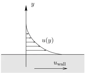
We first assess the accuracy of the current method using a one-dimensional Stokes’ problem where an infinitely long flat plate is impulsively set into motion with

(39)

2.5 Results 25

y

uwall

u(y)

Figure 2.2: Setup for the one-dimensional Stokes’ problem.

uniform grid discretization. The top and bottom boundaries are placed far enough to avoid periodicity from interfering with the velocity profile near the translating plate. Spatial and temporal convergence is analyzed in term of the L∞ and L2 norms of the horizontal velocity error,ej =u(yj)−uj, over the domain yj ∈[0,1] (in non-dimensional length: yj/√νt0∈[0,3.162]).

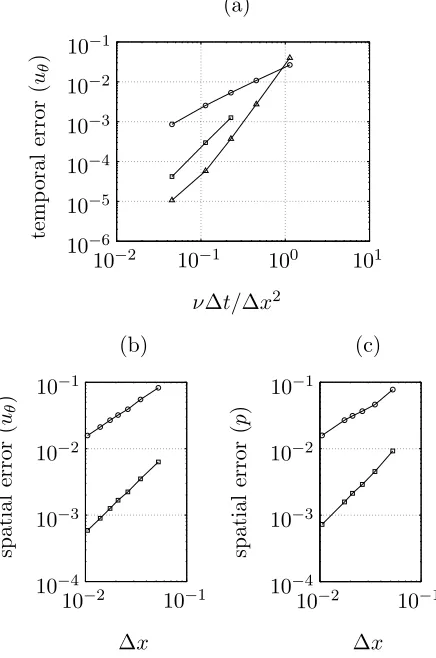
Figure 2.3(a) assesses the temporal L∞ error for various sizes of

non-dimensional time steps, ν∆t/∆y2. The error was computed by comparing the solution to a temporally refined reference solution at fixed grid resolution to isolate the spatial discretization error. We calculate the error att= 0.11 with ∆y= 10−2. The three convergence curves on the plot result from the use of different orders of expansion N forBN (or A−1). Note that the splitting error from Eq. (2.24) is larger in magnitude than the underlying second-order error resulting from the time integration schemes. Hence this splitting error directly influences the temporal accuracy for the range of ∆tconsidered. As discussed in Perot (1993), the splitting error cannot be absorbed by λ because LM−1 and Q are not commutative even for a periodic domain.

(40)

(a) (b) te m p or al er ro r ( u

) 10−1

10−2 10−3 10−4 10−5 10−6

10−2 10−1 100 101

sp at ia l er ro r ( u ) 10 −1 10−2 10−3 10−4 10−5

10−3 10−2 10−1

ν∆t/∆y2 ∆y

Figure 2.3: Error norms from the one-dimensional Stokes’ problem. (a)

TemporalL∞norm errors with different orders of expansion,N, forA −1

;N= 1:

, N = 2: , and N = 3: _△. (b) The L∞: and L2: spatial velocity error norms.

2.3(b). Fortunately, this smearing effect is dominant only in close proximity of the plate and the underlying second-order convergence is achieved in theL2 sense.

2.5.2

Flow inside two concentric cylinders

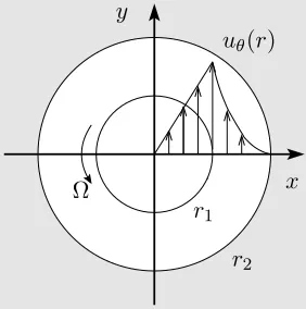
For a two-dimensional test problem, we simulate flow between two concentric hollow cylinders with radii r1 = 1/2 and r2 = 1 as well as the flow inside the smaller cylinder as shown in Figure 2.4. The outer cylinder is held stationary while the inner cylinder is rotated with angular velocity Ω,

Ω = uθ(r1)

r1

= 1 + tanh

t−0.2 0.05

, (2.41)

moving the initially quiescent fluid at t = 0. We take a periodic computational domain of size [₋1.05,1.05] _×[₋1.05,1.05] with uniform spatial resolution and compute the azimuthal velocity error,ej =uθ(rj)−uθ,j, overrj ∈[0, r2] (including flow inside the inner cylinder) reporting theL∞ and L2 norms.

(41)

2.5 Results 27

x y

uθ(r)

r1

r2 Ω

Figure 2.4: Setup for the problem of two concentric cylinders (inner cylinder

rotates with angular velocity Ω).

convergence by comparing our results to a reference solution obtained with a very fine time step, ∆t = 5_×10−6, and spatial resolution, ∆x = ∆y = 2.1_×10−2. The spatial resolution is kept constant and viscosity is set toν = 1. Figure 2.5(a) shows that the order of expansion N for A−1 again influences the behavior of convergence in a fashion similar to the one-dimensional case. As it can be seen from the N = 3 case, the second-order time integration error starts to affect the total error at the smallest shown time step. Based on both the one- and two-dimensional test problems, we recommend the use of third-order expansion N for practical problems. There also is an advantage in choosing N = 3 for achieving positive-definiteness of the modified Poisson equation with larger choice of ∆t

(Perot, 1993).

(42)

(a) te m p or al er ro r ( uθ ) 10−1

10−2 10−3 10−4 10−5 10−6

10−2 10−1 100 101

ν∆t/∆x2

(b) (c) sp at ia l er ro r ( uθ ) 10−1

10−2

10−3

10−4

10−2 10−1

sp at ia l er ro r ( p ) 10 −1

10−2

10−3

10−4

10−2 ₁₀−1

∆x ∆x

Figure 2.5: Error norms from the problem of two concentric cylinders. (a)

TemporalL∞norm errors with different orders of expansion,N, forA −1

;N= 1:

(43)

2.5 Results 29 The spatial accuracy of the pressure is also studied by comparing the current solution to the exact solution at steady-state. Because the pressure based on the current scheme only solves up to a constant (since we pin the pressure to remove the zero eigenvalue), we compare the solutions by matching the pressure atr = 0 for all cases and compute the error norms along thex-axis from 0 tor1. The infinity and L2 error norms are plotted against the grid size in Figure 2.5(c) for the same problem considered in assessing the spatial accuracy of velocity. As expected, the spatial accuracy follows the same trend as the velocity shown in Figure 5(b). Due to the presence of the discrete Delta function along the immersed boundary, the pressure distribution is affected limiting the spatial accuracy to orders of one and about 1.5 for the infinity and L2 norms, respectively.

2.5.3

Flow over a stationary cylinder

We consider flow over a circular cylinder as another test problem because the dimensions of the recirculation zone and the force on the cylinder at various Reynolds numbers are readily available from previous experimental and numerical studies. For the numerical studies, we list results from the immersed boundary method of Lai & Peskin (2000) and the immersed interface method of Linnick & Fasel (2005) among others when the data are available. Our two-dimensional simulations are performed by introducing a cylinder of diameter d= 1 in a large computational domain D with initially uniform flow, u = u∞ = 1. Reynolds

numbers of Re=u∞d/ν= 20, 40, and 200 are chosen for validating the current

method at steady-state and periodic vortex shedding conditions (νis the kinematic viscosity).

(44)

nx×ny D ∆xmin ∆t CFLmax nB Case A 150_×150 [₋30,30]_×[₋30,30] 0.04 0.005 0.22* 78 Case B 300×300 [−30,30]×[−30,30] 0.02 0.005 0.46* 157 Case C 300_×300 [₋15,45]_×[₋30,30] 0.0333 0.0125 0.81_† 94 Case D 300×300 [−10,10]×[−30,30] 0.0333 0.0125 0.75† 94

Table 2.1: Parameters for spatial and temporal discretization used in the

simulations. The maximum CFL numbers are reported from Re= 40 (*) and

Re= 200 (†) cases.

to ensure that the boundary conditions along ∂D do not influence our solution. Left (inflow) and lateral boundary conditions along ∂_D are set to uniform flow of (u, v) = (u∞,0) and are placed far away from the cylinder. At the outlet, the

convective boundary condition (∂u/∂t+u∞∂u/∂x=0) is applied to allow vorticity

to exit the domain freely. Various spatial and temporal resolutions are chosen to ensure that reliable solutions are obtained. We record the maximum CFL number (CFLmax = umax∆t/∆xmin) in Table 2.1 from cases of Re = 40 and Re = 200. Note that the current method yields a stable solution even with CFLmax= 0.81.

For comparison, we compute the force on the body applied by the flow in terms of the drag and lift coefficients: CD ≡ Fx/1₂ρu2∞d and CL ≡ Fy/1₂ρu2∞d,

respectively, where ρu2

∞d = 1. The force on the cylinder, F, can be obtained

simply by

F(t) =

 Fx(t)

Fy(t)

 =−

Z

x

Z

s

f(ξ(s, t))δ(ξ(s, t)−x)dsdx

≈ −X i

Hi,kfk∆x∆y

(2.42)

using the regularization operator and the boundary forcing function. Summation over iis implied to take place separately for each direction of the force vector.

(45)

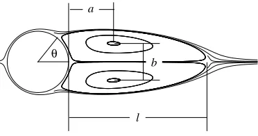
2.5 Results 31

a

b θ

l

Figure 2.6: Definition of the characteristic dimensions of the wake structure.

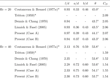
characteristics. The resulting wake dimensions and drag coefficients are compared to values reported in the literature. The size of the wake is characterized byl,a,b, and θ (appropriately non-dimensionalized by the diameter) defined in Figure 2.6 following the notation used in Coutanceau & Bouard (1977a). The parameters,l,

a, and brepresent the length of the recirculation zone, distance from the cylinder to the center of the wake vortex, and the gap between the centers of the wake vortices, respectively. The separation angle is denoted by θmeasured from the x -axis. The steady-state vorticity contours and streamlines from Case B are shown in Figure 2.7 for Re = 20 and 40. The flow profiles are in close agreement with those reported in the literature. The wake properties from Cases A and B are compared against previous experimental and numerical studies in Table 2.2 and are also found to be in accord.

Next, we consider flow over a cylinder at a Reynolds number of 200 to reproduce periodic vortex shedding. A short time after simulations are initiated from uniform flow, a perturbation in a form of an asymmetric body force is added to trigger the shedding instability. Numerical results replicate the periodic shedding of vortices to form the K´arm´an vortex street as shown in the vorticity contour of Figure 2.8. The resulting lift and drag coefficients and the Strouhal number, St _≡ fsd/u∞,

(46)

Re= 20 Re= 40

0

0 2

2

2 4

-0

0 2

2

2 4

-0

0 2

2

2 4

-0

0 2

2

2 4

-Figure 2.7: Vorticity contours (top) for steady-state flow over a cylinder, where

contour levels are set from -3 to 3 in increments of 0.4, and corresponding

(47)

2.5 Results 33

l/d a/d b/d θ CD

Re= 20 Coutanceau & Bouard (1977a)* 0.93 0.33 0.46 45.0◦

-Tritton (1959)* - - - - 2.09

Dennis & Chang (1970) 0.94 - - 43.7◦ 2.05 Linnick & Fasel (2005) 0.93 0.36 0.43 43.5◦ _2.06

Present (Case A) 0.97 0.39 0.43 44.1◦ 2.07 Present (Case B) 0.94 0.37 0.43 43.3◦ _2.06

Re= 40 Coutanceau & Bouard (1977a)* 2.13 0.76 0.59 53.8◦

-Tritton (1959)* - - - - 1.59

Dennis & Chang (1970) 2.35 - - 53.8◦ 1.52 Linnick & Fasel (2005) 2.28 0.72 0.60 53.6◦ _1.54

Present (Case A) 2.33 0.75 0.60 54.1◦ 1.55 Present (Case B) 2.30 0.73 0.60 53.7◦ _1.54

Table 2.2: Comparison of experimental and numerical studies of steady state

wake dimensions and drag coefficient from flow over a cylinder for Re= 20and

(48)

0

0 2

2

2 4 6

-Figure 2.8: Snapshot of the vorticity field with contour levels from -3 to 3 in

increments of 0.4 for Re= 200.

previous findings.

Results from Case D compared to Cases B and C suggest that the placement of the outflow boundary is not too critical. As a pair of positive and negative vortices convect downstream, their effect on the cylinder become less important since their far-field induced velocity would appear to cancel. On the other hand, we have observed pronounced interference from the lateral boundary conditions when the height of the computational domain is shortened.

2.5.4

Flow around a moving cylinder

As our last test problem, we simulate flow around a circular cylinder in impulsive translation to validate the present method for moving bodies. The simulation is performed by moving the Lagrangian body points at each time step. As these points shift their positions in time, the regularization and interpolation operators are updated according to Eq. (2.28). We initially position the cylinder with unit diameter (d= 1) at the origin and impulsively set it into motion to the left with a constant velocity of u0 = −1. Results are presented for Reynolds numbers of

(49)

2.5 Results 35

St CD CL

Re= 200 Belov et al. (1995) 0.193 1.19_±0.042 _±0.64 Liu et al. (1998) 0.192 1.31±0.049 ±0.69 Lai & Peskin (2000) 0.190 -

-Roshko (1954)* 0.19 -

-Linnick & Fasel (2005) 0.197 1.34_±0.044 _±0.69 Present (Case B) 0.196 1.35±0.048 ±0.68 Present (Case C) 0.195 1.34_±0.047 _±0.68 Present (Case D) 0.197 1.36±0.043 ±0.69

Table 2.3: Comparison of Strouhal number and coefficients of drag and lift

for flow over cylinder from experimental and numerical studies at Re = 200.

Experimental studies are listed with (*).

The computational domainD is taken to be [−16.5,13.5]×[−15,15] with no-slip boundary condition applied along∂_D. Non-uniform grid is used with uniform grid in the near field having a resolution of ∆xmin = 0.02 resulting in a grid size of 425_×250. A constant time step of ∆t = ∆xmin/2 is chosen such that the maximum CFL numbers are limited to 0.98 and 0.81, respectively forRe= 40 and 200 during the simulation from a non-dimensional time of t∗_{≡ |}u0|t/d= 0 to 3.5. Quiescent flow is used for the initial condition.

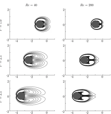
We present snapshots of the flow field at non-dimensional time oft∗ = 1, 2.5, and 3.5 in Figure 2.9. Left and right figures illustrate the vorticity field forRe= 40 and 200, respectively. The flow fields are in agreement with those in Coutanceau & Bouard (1977b) and Koumoutsakos & Leonard (1995) forRe= 40. ForRe= 200, the flow exhibits a generation of stronger vortex pair in the wake of the cylinder. In the two cases, the solutions are resolved well even near the boundary and the difference in the effect of viscous diffusion is nicely captured.

(50)

Re= 40 Re= 200

t

∗ =

1

.

0

0 2

2 ₄ ₂

- _-

-0

0 2

2 ₄ ₂

- _-

-t

∗ =

2

.

5

0

0 2

2 ₄ ₂

- _-

-0

0 2

2 ₄ ₂

- _-

-t

∗ =

3

.

5

0

0 2

2 ₄ ₂

- _-

-0

0 2

2 ₄ ₂

- _-

-Figure 2.9: Snapshots of the vorticity field around an impulsively moving

circular cylinder for Re= 40and 200at non-dimensional time oft∗

= 1,2.5, and

(51)

2.5 Results 37

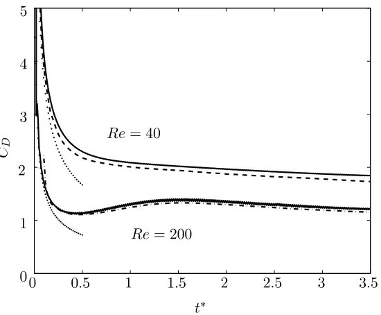
CD

0 0.5 1 1.5 2 2.5 3 3.5

0 1 2 3 4 5

Re= 40

Re= 200

t∗

Figure 2.10: History of the drag coefficient of the body for Re = 40 and 200

( ) compared with numerical solutions from Koumoutsakos & Leonard

(1995) (Re= 40, ) and Cottetet al._{(2000) (}_Re_{= 200}_, _{) and analytical}

solution by Bar-Lev & Yang (1997) ( ) valid for early time.

vortex methods from Koumoutsakos & Leonard (1995) and Cottet et al. (2000) along with the analytical series solution by Bar-Lev & Yang (1997) valid for early time are superposed on the current results. The current scheme reveals the singular behavior of the drag at the start up time (O(1/√t∗_{)) experienced by the cylinder}

due to the impulsive motion (Bar-Lev & Yang, 1997). Our drag coefficients are about 4 to 5% larger than those from the vortex method. Additional simulations were performed with smaller grid spacings and larger computational domains. However, there were no noticable changes in our solutions to account for the difference.

We also measure the length of the recirculation zone, previously defined asl/d

(52)

(a)Re= 40 (b)Re= 200

l/

d

0 1 2 3

0 0.5 1 1.5

l/

d

0 1 2 3

0 0.5 1 1.5

t∗ t∗

Figure 2.11: Length of the recirculation zone, l/d, in the frame of reference

of the moving cylinder as a function time, t∗

, for (a) Re = 40 and (b)

Re= 200compared with previous studies. Present results: ; experimental

measurements of Coutanceau & Bouard (1977b_{) (}_Re _{= 40}_, _{); and}

numerical study of Collins & Dennis (1973) (Re= 200, ).

Coutanceau & Bouard (1977b) and are found to be in excellent agreement shown by the overlaps for both Reynolds numbers.

2.5.5

Flow over a sphere

The current method has been extended to three dimensions as well. We present some validation performed for flow around a sphere at steady state.

(53)

2.6 Summary 39

l/d a/d b/d θ CD

Re= 100 Present 0.91 0.28 0.59 50.4◦ _1.14

Johnson & Patel (1999) 0.88 0.25 0.60 53◦ 1.10

Re= 200 Present 1.38 0.37 0.69 61.2◦ 0.82 Johnson & Patel (1999) 1.46 0.39 0.74 63◦ 0.80

Table 2.4: Steady-state wake dimensions and drag coefficient from flow over a

sphere at Re= 100 and 200.

y

-1 0 1 2 3

-1 -0.5 0 0.5 1

x

Figure 2.12: Steady-state vorticity field around a sphere at Re= 200. Contour‘

levels are set from −3 to 3 in increments of 0.4. Negative contour levels are

shown with dashed lines.

Johnson & Patel (1999).

Three-dimensional validation of unsteady flows are offered later in Section 3.2.2 for flows over an impulsively translating low-aspect-ratio flat-plate wing at Re = 100.

2.6

Summary

(54)

(55)

41

Chapter 3

Separated Flows around

Low-Aspect-Ratio Wings

3.1

Introduction

(56)

spanwise circulation resulting in enhanced lift. Such forces applied by the unsteady vortex formation in two-dimensional flows were investigated both experimentally by Dickinson & G¨otz (1993) and numerically by Wang (2000a,b, 2004) and Bos et al. (2008). Furthermore, the full three-dimensional studies drawing attention to spanwise flows and tip effects around the flapping wings were undertaken experimentally by Ellington et al. (1996), Birch & Dickinson (2001), Usherwood & Ellington (2002), Birch et al. (2004), and Poelma et al. (2006). Analogous numerical studies were performed by Liu et al. (1998) and Sun (2005).

Similar investigations have been carried out to analyze the efficient locomotion of swimming animals. In particular, von Ellenrieder et al. (2003), Buchholz & Smits (2006), and Parker et al. (2007) have visualized the wake vortices behind flapping low-aspect-ratio hydrofoils to understand the qualitative dynamics. Numerical simulations of the three-dimensional flows over flapping foils were also performed by Blondeaux et al. (2005) and Dong et al. (2006) at Reynolds numbers similar to the present study. Moreover, Drucker & Lauder (1999) have experimentally visualized the flows around pectoral fins and Zhuet al.(2002) have performed simulations around an entire fish to identify the wake structures.

For purely translating low-aspect-ratio wings, Torres & Mueller (2004) have experimentally measured the aerodynamic characteristics of low-aspect-ratio wings at Reynolds numbers around 105. Aerodynamic performance (lift, drag, pitching moment, etc) of various planforms was considered over angles of attack (α) of 0◦ to 40◦ and aspect ratios (AR) of 0.5 to 2 and was observed to be quite different from that of low-aspect-ratio wings in high-Reynolds-number flows. They concluded that the most important parameter that influences the aerodynamic characteristics is the aspect ratio. Transient studies have also been conducted by Freymuth et al. (1987) by using smoke to visualize the start-up flows around low-aspect-ratio airfoils. A qualitative insight into the three-dimensional formation of wake vortices was presented. The experiments by Ringuette et al. (2007) extensively studied the wake vortices behind low-aspect-ratio plates but only at α= 90◦_.

(57)

3.2 Simulation methodology 43 were performed by Hamdani & Sun (2000). Also, studies by Mittal & Tezduyar (1995) and Cosyn & Vierendeels (2006) considered the three-dimensional flows around translating low-aspect-ratio planforms but focused mostly on those at low angles of attack. For wings at post-stall angles of attack, unsteady separated flows and vortex dynamics behind low-aspect-ratio wings in pure translation are still not well-documented.

To extend the previous studies, we use numerical simulations to examine the aerodynamics of impulsively started low-aspect-ratio flat-plate wings under pure translation at Reynolds numbers of 300 and 500. These Reynolds numbers are high enough to induce separation and unsteadiness in the wake but low enough for the three-dimensional flow field to remain laminar. The regime also includes, for a range of angles of attack, the critical Reynolds numbers at which the flow first becomes unstable to small disturbances. In the following section, we present the numerical method and its validation. In Section 3.3, results from separated flows around the airfoils are presented. We call attention to the transient nature of the flow field and its influence on the aerodynamic forces. The stability of the wake is also investigated at large time. Dynamics of the wake vortices and the corresponding lift and drag are considered over a range of angles of attack and various planform geometries.

3.2

Simulation methodology

3.2.1

Simulation setup

(58)

non-dimensionalized by the chord (c) of the plate. Grid stretching is applied in all directions with finer resolution near the plate to capture the wake structure as illustrated in Figure 3.1. Extensive studies have been performed in two and three dimensions to ensure that the present choice of grid resolution and domain size does not influence the flow field in a significant manner (previously reported in Taira et al.(2007)).

Boundary conditions along all sides of the computational boundary, ∂D, are set to uniform flow (U∞,0,0) except for the outlet boundary where a convective

boundary condition (∂u

∂t + U∞ ∂u

∂x = 0) is specified. Inside the computational domain, a flat plate is positioned with its center at the origin. This flat plate is instantaneously materialized at t= 0+ in an initially uniform flow to model an impulsively started translating plate. Computations are advanced in time with a time step such that the Courant number based on the free-stream velocity obeys

U∞∆t/∆x ≤ 0.5. Both the initial transient and the large-time behavior of the

flow are considered. The time variable is reported in terms of the nondimensional convective time unit (i.e. ,U∞t/c).

In Chapters 3 and 4, the Reynolds number is defined as Re _≡U∞c/ν, where

ν denotes the kinematic viscosity of the fluid. Forces on the flat plate (Fx, Fy, Fz) are described in terms of the non-dimensionalized lift, drag, and side forces defined by CL=Fy/(1₂ρU∞2 A), CD =Fx/(1₂ρU∞2A), andCS =Fz/(1₂ρU∞2 A), respectively,

where ρ is the density of the fluid and A is the area of the flat plate. In the case of two-dimensional flows, the force per unit span is normalized by the chord.

3.2.2

Validation

We compare results from the three-dimensional simulations and measurements from an oil tow-tank experiment1 of flows over a rectangular plate ofAR = 2 at

(59)

3.2 Simulation methodology 45

x y

z

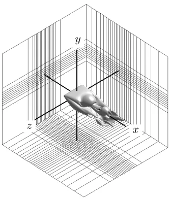
Figure 3.1: A typical computational domain showing the top-port side of the

wake around a rectangular flat plate of AR= 2. The spatial discretization of

this computational domain is shown for every 5 cells for thex- andy-directions

and every 4 cells for the z-direction.

is of dimension 82mm _× 164mm _× 3mm and is rigidly mounted to a six-axis force sensor at one wing tip to limit lift due to backlash in the gearbox. This setup is attached to a translation sled equipped with a servo motor providing control of the translati