Volume 2008, Article ID 417157,7pages doi:10.1155/2008/417157
Research Article
Decoupled Estimation of 2D DOA for Coherently Distributed
Sources Using 3D Matrix Pencil Method
Zhang Gaoyi and Tang Bin
School of Electronic Engineering, University of Electronic Science and Technology of China, Chengdu 610054, China
Correspondence should be addressed to Zhang Gaoyi,[email protected] Received 31 January 2008; Revised 17 May 2008; Accepted 13 July 2008
Recommended by S. Gannot
A new 2D DOA estimation method for coherently distributed (CD) source is proposed. CD sources model is constructed by using Taylor approximation to the generalized steering vector (GSV), whereas the angular and angular spread are separated from signal pattern. The angular information is in the phase part of the GSV, and the angular spread information is in the module part of the GSV, thus enabling to decouple the estimation of 2D DOA from that of the angular spread. The array received data is used to construct three-dimensional (3D) enhanced data matrix. The 2D DOA for coherently distributed sources could be estimated from the enhanced matrix by using 3D matrix pencil method. Computer simulation validated the efficiency of the algorithm.
Copyright © 2008 Z. Gaoyi and T. Bin. This is an open access article distributed under the Creative Commons Attribution License, which permits unrestricted use, distribution, and reproduction in any medium, provided the original work is properly cited.
1. INTRODUCTION
In many applications, such as wireless communications,
radar, and sonar, the effect of angular spread can no
longer be ignored. A distributed source model will be
more appropriate [1, 2]. Distributed source is classified
as coherently distributed (CD) source and incoherently
distributed (ICD) source in literature [2], where angular
signal density of the sources is used to form the distributed model. When the received signal components from a source
at different angles are delayed and scaled replicas of the
same signal, the source is called coherently distributed.
When the signal rays arriving from different directions are
uncorrelated, the source is called incoherently distributed. In CD source case, the rank of the noise-free covariance matrix is equal to the number of sources. Some classical
estimation methods [2–6] were generalized from the case
of point sources to the case of CD sources. DSPE [2, 6]
is generalized from MUSIC for the distributed sources parameter estimation. ESPRIT is extended for distributed sources parameter estimation by using two closely-spaced
ULAs [3]. The above algorithms have mainly been developed
for azimuth-only estimation and angular spread. Based on two closely-spaced UCAs, the sequential one-dimensional
searching (SOS) method [4] which is the combination
of ESPRIT and alternate minimization in 2D problem is
developed in [4], where the nominal azimuth DOA and
elevation DOA of coherently distributed sources can be obtained by one-dimensional search. Based on specially designed array geometry, VESPA is used for the estimation of 2D DOA and angular spread for coherently distributed
source [5].
In this paper, the Taylor approximation is used to separate the angular information from angular spread information. The angular information can be got from the phase part of the received signal, which can be got from the poles extracted by matrix pencil (MP) method. So, MP method can be used to decouple the estimation of 2D DOA from that of the angular spread for coherently distributed source. The MP method is used for the estimation of
two-dimensional frequencies in [7,8] and then extended for the
2D DOA estimation for point source in [9,10]. We extend
x
. ..
2σφ
φ
2σθ
θ · · · y z
. . .
Figure1: Array geometry.
2. SIGNAL MODEL
Assume that stationary signals impinge on an array of K
sensors fromI narrowband far-field sources. The output of
the sensors of the array is given by
v(t)=Bs(t) +n(t), (1)
where B = [b1,b2,. . .,bI], s(t) = [s1(t),s2(t),. . .,sI(t)]T,
and n(t), respectively, are the K ×I generalized steering
matrix formed between the sources and the antenna elements
at the array, theI×1 signal vector transmitted by the source,
and theK×1 additive noise vector.biis theK×1 GSV of the
ith CD source, which is defined as
bi=
a(θ,φ)ρ(θ,φ;μi)dθ dφ, (2)
wherea(θ,φ) is the steering vector for a point source at 2D
DOA (θ,φ),μi =(θi,σθi,φi,σφi) is a vector whose elements,
respectively, are the azimuth DOA, the angular spread of the azimuth DOA, the elevation DOA, and the angular spread
of the elevation DOA of the ith CD source. ρ(θ,φ;μi) is
the deterministic angular weighting function of theith CD
source.
Similar to [4], when the angular spread is small, for a
single CD source narrowband centered in λ, we can use
the Taylor approximation, the elements of GSV can be approximately decomposed as
bk(μ)=
b(θ,σθ,φ,σφ)
k≈
a(θ,φ)]k[g(θ,σθ,φ,σφ)
k, (3)
where [a(θ,φ)]k is the phase part of the GSV, and
[g(θ,σθ,φ,σφ)]kis the module part of the GSV.
Consider a three-dimensional array in space as illustrated in Figure 1 with the axes oriented along the Cartesian
coordinates. The distances between the elements areΔx,Δy,
andΔz, which are always half of the wavelength.
The number of sensors areA,B, andCsatisfyingA+B+
C=K. Therefore, we have
[a(θ,φ)](a,b,c)
=ej((2π/λ)Δxcosθcosφa+(2π/λ)Δysinθcosφb+(2π/λ)Δzsinφc), (4)
wherea=1,. . .,A;b=1,. . .,B;c=1,. . .,C; and
[g(θ,σθ,φ,σφ)](a,b,c)Gaussian
=e−2π2σ2θ(−Δxsinθcosφa+Δycosθcosφb)2/λ2
×e−2π2σ2
φ(−Δxcosθsinφa−Δysinθsinφb+Δzcosφc)2/λ2
(5)
for Gaussian shaped coherently distributed (GCD) source,
[g(θ,σθ,φ,σφ)](a,b,c)Laplacian
=1/1 + 2(πσθ(−Δxsinθcosφa+Δycosθcosφb)/λ)2)
×(1 + 2(πσφ(−Δxcosθsinφa−Δysinθsinφb
+Δzcosφc)/λ)2
(6)
for Laplacian shaped coherently distributed (LCD) source. It is noted that when the angular spread of coherently distributed source is small, for Gaussian shaped and Lapla-cian shaped distributed source, the angular information and angular spread information could be separated from the
signal pattern. From (3), (4), (5), and (6), we know that the
angular spread only affect the module of the received signal
because MP algorithm extracts the poles from the phase of signal, the MP algorithm might be used for the estimation
of 2D DOA similar as [9] for point source. For differently
shaped coherently distributed source, the 2D DOA can be decoupled from the angular spreads by using MP algorithm. So, the MP algorithm can obtain the 2D DOA of coherently distributed sources without the prior information of the shape of the angular weighting function. Obviously, when
σθ =0 andσφ=0, the above model is a point model. When
the angular spread increases, the module of the coherently distributed sources decreases.
3. MATRIX PENCIL METHOD
Assume the ith coherently distributed source signals are
narrowband centered inλi, consider a 3D data cube as
v(a;b;c)
=
I
i=1
ej((2π/λi)Δxcosθicosφia+(2π/λi)Δysinθicosφib+(2π/λi)Δzsinφic)α
i
+w(a,b,c),
(7)
wherew(a,b,c) denotes the noise, and
wheresi(t)=Miejγiis the signal with amplitude ofMialong
with the phaseγi.
Define 3D polesxi,yi, andzias follows:
xi=exp
j2π
λiΔxcosθicosφi
,
yi=exp
j2π
λiΔysinθicosφi ,
zi=exp
j2π
λiΔzsinφi .
(9)
After the poles are found, the elevation and the azimuth angle are obtained for each source as follows:
Gi=angle(xi
)
2πΔx , Ei=
angle(yi)
2πΔy , Fi=
angle(zi)
2πΔz ,
(10)
θi=arctan
Ei
Gi , (11)
φi=arctan
Fi
G2
i +E2i
. (12)
The 3D data matrix can be enhanced by using the
partition and stacking process. The column vectors along
x-direction are enhanced by a pencil parameterLand they are
stacked to getDy,zas follows:
Dy,z
= ⎡ ⎢ ⎢ ⎢ ⎢ ⎣
v(0;y;z) v(1;y;z) · · · v(A−L;y;z)
v(1;y;z) v(2;y;z) · · · v(A−L+ 1;y;z) ..
. ... . .. ...
v(L−1;y;z) v(L;y;z) · · · v(A−1;y;z) ⎤ ⎥ ⎥ ⎥ ⎥ ⎦
L(A−L+1)
.
(13)
The matrixDy,zis enhanced along y-direction with the
pencil parameterMas follows:
Dz= ⎡ ⎢ ⎢ ⎢ ⎢ ⎣
D0,z D1,z · · · DB−M,z D1,z D2,z · · · DB−M+1,z
..
. ... . .. ...
DM−1,z DM,z · · · DB−1,z ⎤ ⎥ ⎥ ⎥ ⎥ ⎦
LM(A−L+1)(B−M+1)
.
(14)
The matrix Dz is enhanced along z-direction with the
pencil parameterNas follows:
De= ⎡ ⎢ ⎢ ⎢ ⎢ ⎣
D0 D1 · · · DC−N
D1 D2 · · · DC−N+1
..
. ... . .. ...
DN−1 DN · · · DC−1
⎤ ⎥ ⎥ ⎥ ⎥ ⎦
LMN(A−L+1)(B−M+1)(C−N+1)
.
(15)
The enhanced data matrixDe is used to obtain the 3D
poles [9]. The singular value decomposition of matrixDehas
the form
De=USΛSVHS +UnΛnVHn, (16)
where H denotes the conjugate transpose, the subindexes
S and n stand for the signal and noise components,
respectively.
As discussed in [9], the pencil parameter must be chosen
to satisfy two relationships with the number of signal as follows:
LMN ≥I,
(A−L+ 1)(B−M+ 1)(C−N+ 1)≥I. (17)
In CD source case, the rank of the noise-free covariance matrix is equal to the number of sources. The algorithm can be summarized as follows.
Step 1. Form theLMN×(A−L+ 1)(B−M+ 1)(C−N+ 1)
enhanced matrixDefrom the noisy data according to (15).
Step 2. Compute the singular values and the left singular
vectorsUsofDe. Estimate the number of the sources from
the singular values.
Step 3. Estimate the polesxi,yi, andzifromUsand pair the
poles as illustrated in [9].
Step 4. Estimate the 2D DOA of coherently distributed
source from the poles by using (11) and (12).
The MP algorithm for 2D DOA estimation only used the phase information of the signal. It can be inferred that the angular spread can be got from the module information of the signal with some prior information of the angular
weighting function. From literature [9], the wavelength can
be got from the estimated poles. However, for simplicity, in this paper, the 2D DOA estimation problem for coherently distributed sources is focused.
4. CRAMER-RAO BOUND
The Cramer-Rao bound (CRB) for the point source could
be seen in [9]; the CRB for coherently distributed source is
derived as follows.
Consider the sampled values of the noise contaminated
signal v. Assume that the noise is complex Gaussian, the
probability density function ofvis
P(v/ϕ)= 1
(2πκ)ABCe
((−1/κ)v−v2
), (18)
where·denotes the 2-norm,κis the variance of the noise,
andϕis theI×1 column vector of the unknown parameters
defined as follows:
ϕ=ϕ1 ϕ2 · · · ϕI T
,
ϕi=
Mi γi λi θi φi σθi σφi
T
.
(19)
The element of the 7I×7I Fisher information matrixF
is defined by
Fi j= −E
∂2
∂ϕi∂ϕj log(p(v/ϕ))
0 0.1 0.2 0.3 0.4
RMSE
o
f
azim
u
th
ang
le
(deg)
0 5 10 15 20 25
SNR (dB) MP for GCD source 1 MP for GCD source 2
CRB for GCD source 1 CRB for GCD source 2 Figure2: RMSE of azimuth angle for GCD sources.
where Fi j is a 7×7, (i,j)th block matrix of F. E{·} is
the expectation operator,∂/∂ϕiis the partial derivative with
respect to the ith element ϕi of ϕ, and log is the natural
logarithm. Using (18) in (20), we have
Fi j=1
κ2Re
∂vH
∂ϕi
∂v ∂ϕj
, (21)
where Re(·) denotes the real part.
By using the Fisher information matrix, the Cramer-Rao bound (CRB) is defined as
var(ϕi)≥[F−1(ϕ)]
ii. (22)
So the variance of the unbiased estimate of the ith
parameter is theith diagonal element of the inverse of the
Fisher information matrix. Thus, we can compare the RMSE
of the MP algorithm withvar(ϕi) to measure the goodness
of the estimator.
5. NUMERICAL RESULTS
In this section, we provide numerical illustrations of the performance of the proposed algorithm. We assume all of the signals are equipower and have the same frequency. The
numbers of the array elements in x-direction, y-direction,
and z-direction are all 10, the distance between adjacent
sensors is λ/2. It is assumed that all the signals impinging
on the array with amplitudesMi=1 and phasesγi=0. The
results are based on 500 Monte Carlo simulations.
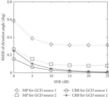
In the first example, we illustrate the performance of MP
algorithm for two GCD source one withμ1=(35, 3.5, 40, 4)
and another one with μ2 = (25, 2.5, 20, 2). The pencil
parameters are all 4. We compare with the CRB for 2D DOA estimation of Gaussian shaped coherently distributed
source. Figures2and3show that the RMSE of the estimators
approaches the CRB when SNR varies from 0 dB to 25 dB.
0 0.2 0.4 0.6 0.8
RMSE
o
f
ele
vation
ang
le
(deg)
0 5 10 15 20 25
SNR (dB) MP for GCD source 1 MP for GCD source 2
CRB for GCD source 1 CRB for GCD source 2 Figure3: RMSE of elevation angle for GCD sources.
0 0.5 1 1.5
RMSE
o
f
azim
u
th
ang
le
(deg)
0 5 10 15 20 25
SNR (dB) MP for LCD source 1 MP for LCD source 2
CRB for LCD source 1 CRB for LCD source 2 Figure4: RMSE of azimuth angle for LCD sources.
The RMS errors for the two GCD sources using MP are all smaller than 1 degree when the SNR at 0 dB.
In the second example, we illustrate the performance
of MP algorithm for two LCD source, one with μ1 =
(35, 3.5, 40, 4) and another one withμ2 = (25, 2.5, 20, 2).
The pencil parameters are all 4. Figures4 and5 show that
the RMSE of the estimators approaches the CRB when SNR varies from 0 dB to 25 dB. The RMS errors for the two LCD source using MP are smaller than 1 degree when the SNR at 0 dB.
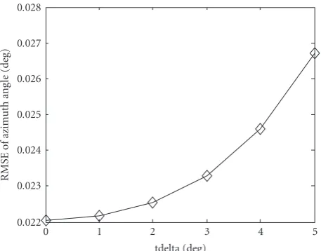
In the third example, we first illustrate the performance
of MP algorithm when θ = 35◦,φ = 40◦,σφ = 4◦, the
angular spread σθ varies, the pencil parameters are all 4,
and SNR is 10 dB: it is observed that the variation of RMSE
of azimuth angle is rather small even when σθ (tdelta in
0 0.2 0.4 0.6 0.8
RMSE
o
f
ele
vation
ang
le
(deg)
0 5 10 15 20 25
SNR (dB) MP for LCD source 1 MP for LCD source 2
CRB for LCD source 1 CRB for LCD source 2 Figure5: RMSE of elevation angle for LCD sources.
0.022 0.023 0.024 0.025 0.026 0.027 0.028
RMSE
o
f
azim
u
th
ang
le
(deg)
0 1 2 3 4 5
tdelta (deg)
Figure6: RMSE of azimuth angle versusσθ.
algorithm when θ = 35◦,φ = 40◦,σθ = 4◦, the angular
spread σφ varies, also the pencil parameters are all 4, and
SNR is 10 dB: it is observed that the variation of RMSE of
elevation angle is also rather small even whenσφ(fdelta in
Figure 7) increases.
Clearly, the MP algorithm provides good estimation accuracy for estimating the nominal azimuth and elevation DOA of coherently distributed source. Note that because the angular information of coherently distributed source is separated from angular spread information, the estimation of the 2D DOA does not need the information of the shape of angular weighting function.
6. CONCLUSIONS
In this study, the coherently distributed source with 3D data cube is constructed using the Taylor approximation, whereas the angular and the angular spread information is
0.085 0.09 0.095 0.1 0.105 0.11 0.115
RMSE
o
f
ele
vation
ang
le
(deg)
0 1 2 3 4 5
fdelta (deg)
Figure7: RMSE of elevation angle versusσφ.
separated from the signal pattern. The matrix pencil method is extended to the estimation of 2D DOA for coherently distributed sources without any search. 3D data matrix is constructed to estimate poles of 3D plane, the azimuth and elevation of each signal could be obtained from the
poles. This method could deal with differently shaped small
angular spread coherently distributed sources without the prior information of the shape of the angular weighting
function. Computer simulation validated the efficiency of
the method. The estimation performance of different shaped
coherently distributed source is studied. The RMS errors of the estimator have been compared with the CRB to observe the goodness of the method at low SNR.
APPENDIX
APPROXIMATION TO THE STEERING VECTOR FOR SMALL ANGULAR SPREADS
From (2), we have
[b(μ)]=[b(θ,σθ,φ,σφ)]
=
[a(ϑ,ϕ)]ρ(ϑ,ϕ;μ)dϑ dϕ
=
ej2π(Δxcosθcosφa+Δysinθcosφb+Δzsinφc)/λ
×ρ(ϑ+θ,ϕ+φ;μ)dϑ d ϕ,
(A.1)
where μ = (θ,σθ,φ,σφ) characterizes the complex source
together with the angular weighting functionρ(ϑ,ϕ;μ) which
shows the angular spreading of the source, for instance, the Gaussian shaped angular weighting function can be expressed as
ρ(ϑ,ϕ;μ)= 1
2πσθσφe
−1/2((ϑ−θ)2/σ2
θ+(ϕ−φ)
2 /σ2
φ). (A.2)
For small values of variablesϑ=ϑ−θandϕ=ϕ−φ, the
by the first terms in the Taylor series expansions. Using the
trigonometric identity cos(α+β) = cosαcosβ−sinαsinβ
and sin(α+β)=sinα·cosβ+ cosαsinβ, we have
ej2π(Δxcos(θ+ϑ)cos(φ+ϕ)a+Δysin(θ+ϑ)cos(φ+ϕ)b+Δzsin(φ+ϕ)c)/λ
=ej2π(Δxcos(θ+ϑ)cos(φ+ϕ)a)/λ
×ej2π(Δysin(θ+ϑ)cos(φ+ϕ)b)/λ×ej2π(Δzsin(φ+ϕ)c)/λ
≈ej2π(Δx(cosθ−ϑsinθ)(cosφ−ϕsinφ)a)/λ
×ej2π(Δy(sinθ+ϑcosθ)(cosφ−ϕsinφ)b)/λ
×ej2π(Δz(sinφ+ϕcosφ)c)/λ
ej2π(Δxcos(θ)cos(φ)a+Δysin(θ)cos(φ)b+Δzsin(φ)c)/λ
×ej2πϑ(−Δxsinθcosφa+Δycosθcosφb)/λ
×ej2πϕ(−Δxcosθsinφa−Δysinθsinφb+Δzcosφc)/λ,
(A.3)
where we assume that ϑϕ ≈ 0 and consequently
ej2πϑϕsinθsinφ/λ1,ej2πϑϕcosθsinφ/λ1. Thus, we can rewrite
(A.1) as
b(θ,σθ,φ,σφ)≈a(θ,φ)g(θ,σθ,φ,σφ), (A.4)
or
[b(θ,σθ,φ,σφ)](a,b,c) ≈[a(θ,φ)](a,b,c)[g(θ,σθ,φ,σφ)](a,b,c),
(A.5)
where
[g(θ,σθ,φ,σφ)](a,b,c)
=
ej2πϑ(−Δxsinθcosφa+Δycosθcosφb)/λ
×ej2πϕ(−Δxcosθsinφa−Δysinθsinφb+Δzcosφc)/λ
×ρ(ϑ+θ,ϕ+φ;μ)dϑ d ϕ.
(A.6)
For Gaussian shaped angular weighting function, we have
[g(θ,σθ,φ,σφ)](a,b,c)
= 1
2πσθσφ
ej2πϑ(−Δxsinθcosφa+Δycosθcosφb)/λe−(ϑ2/2σθ2)dϑ
×
ej2πϕ(−Δxcosθsinφa−Δysinθsinφb+Δzcosφc)/λe−(ϕ2/2σ2
φ)dϕ
=e−2π2σθ2(−Δxsinθcosφa+Δycosθcosφb)2/λ2
×e−2π2σ2
φ(−Δxcosθsinφa−Δysinθsinφb+Δzcosφc)2/λ2,
(A.7)
where the integral formula−∞∞ e−q2x2
ej p(x+λ)dx = √πej pλ·
e−(p2/4q2)
/qis used.
Similarly, when the angular weighting function is Lapla-cian shaped:
ρ(ϑ,ϕ; μ)= 1
2σθσφe
−(√2|ϑ−θ|/σθ+
√
2|ϕ−φ|/σφ), (A.8)
we have
[b(θ,σθ,φ,σφ)](a,b,c)
≈[a(θ,φ)](a,b,c)[g(θ,σθ,φ,σφ)](a,b,c)
[a(θ,φ)](a,b,c)
×
1
√
2σθ
ej2πϑ(−Δxsinθcosφa+Δycosθcosφb)/λe−(√2|ϑ|/σθ)dϑ
×
1
√
2σφ
ej2πϕ(−Δxcosθsinφa−Δysinθsinφb+Δzcosφc)/λ
×e−(√2|ϕ|/σφ)dϕ
[a(θ,φ)](a,b,c)
×1/1 + 2(πσθ(−Δxsinθcosφa+Δycosθcosφb)/λ)2
×1/1 + 2(πσφ(−Δxcosθsinφa−Δysinθsinφb
+Δzcosφc)/λ)2
(A.9)
using 0∞e−pxcos(vx+ε)dx = (pcosε−vsinε)/(p2+v2),
p >0.
REFERENCES
[1] P. Zetterberg,Mobile cellular communications with base station antenna arrays: spectrum efficiency, algorithms and propagation models, Ph.D. dissertation, Signals, Sensors, Systems Depart-ment, Royal Institute of Technology, Stockholm, Sweden, 1997.
[2] S. Valaee, B. Champagne, and P. Kabal, “Parametric local-ization of distributed sources,” IEEE Transactions on Signal Processing, vol. 43, no. 9, pp. 2144–2153, 1995.
[3] S. Shahbazpanahi, S. Valaee, and M. H. Bastani, “Distributed source localization using ESPRIT algorithm,”IEEE Transac-tions on Signal Processing, vol. 49, no. 10, pp. 2169–2178, 2001. [4] J. Lee, I. Song, H. Kwon, and S. R. Lee, “Low-complexity estimation of 2D DOA for coherently distributed sources,” Signal Processing, vol. 83, no. 8, pp. 1789–1802, 2003. [5] G. Y. Zhang and T. Bin, “Estimation of 2D-DOAs and angular
spreads for coherently distributed sources using cumulants,” inProceedings of the 8th IEEE Workshop on Signal Processing Advances in Wireless Communications (SPAWC ’07), pp. 1–5, Helsinki, Finland, June 2007.
[6] A. Zoubir and Y. Wang, “Efficient DSPE algorithm for estimating the angular parameters of coherently distributed sources,”Signal Processing, vol. 88, no. 4, pp. 1071–1078, 2008. [7] Y. B. Hua, “Estimating two-dimensional frequencies by matrix enhancement and matrix pencil,”IEEE Transactions on Signal Processing, vol. 40, no. 9, pp. 2267–2280, 1992.
[8] Y. B. Hua and T. K. Sarkar, “Matrix pencil method for estimating parameters of exponentially damped/undamped sinusoids in noise,”IEEE Transactions on Acoustics, Speech, and Signal Processing, vol. 38, no. 5, pp. 814–824, 1990.
incoming signals,”Digital Signal Processing, vol. 16, no. 6, pp. 796–816, 2006.