Adaptive Peak Frequency Estimation Using
a Database of PARCOR Coefficients
Tetsuya Watanabe
Department of Communications Engineering, Graduate School of Engineering, Osaka University, Suita 565-0871, Japan
Email:[email protected]
Youji Iiguni
Department of Systems Innovation, Graduate School of Engineering Science, Osaka University, Toyonaka 560-8531, Japan
Email:[email protected]
Received 10 March 2004; Revised 23 July 2004; Recommended for Publication by Chin-Hui Lee
This paper presents an adaptive peak frequency estimation method using a database that stores PARCOR coefficients as key at-tributes and the corresponding peak frequencies as nonkey atat-tributes. The least-square lattice algorithm is used to recursively estimate the PARCOR coefficients to adapt to changing circumstances. The nearest neighbor to the current PARCOR coefficient is retrieved from the database, and the corresponding peak frequency is regarded as the estimation. A simultaneous execution of database construction and peak estimation with database update is performed to accelerate the processing time and to improve the estimation accuracy.
Keywords and phrases:peak frequency, database retrieval, AR spectrum, PARCOR coefficient, adaptive estimation.
1. INTRODUCTION
Estimation of peak frequency of the power spectrum plays an important role in direction-of-arrival estimation, com-munication system, fault diagnosis, and speech processing. Direction-of-arrival of multiple wave sources arriving on a linear array antenna can be estimated by finding local max-ima of the space spectrum obtained from the array inputs [1]. Also in biological signals such as electroencephalogram, blood pressure, heart rate, and laser Doppler flow, peak fre-quencies provide important information on the diagnosis of diseases [2,3,4,5]. Peak frequencies of speech signals are an important cue in the characterization of speech sounds since they have a close relation to the phonetic content. Therefore, extensive studies on peak frequency estimation have been conducted for many years [6,7,8,9,10,11,12,13].
There are two approaches to power spectrum estima-tion: nonparametric estimation methods and parametric es-timation methods. The FFT (fast Fourier transform) method is a representative one of the nonparametric methods, and the AR (autoregressive) method is a representative one of the nonparametric methods. The FFT method estimates the power spectrum directly from the data. The FFT method is very fast, however, the estimation error variance increases as the number of observations decreases. Moreover, the
computationally expensive peak picking is necessary for ex-tracting peak frequencies from the FFT spectrum. The AR method estimates the AR parameters and characterizes the power spectrum by the AR parameters. The AR method pro-vides high-resolution spectrum even with a small number of observations [14]. However, polynomial root finding or peak picking is necessary for extracting peak frequencies from the AR spectrum.
When signal statistics change with time as often happen in real applications, adaptive estimation of peak frequencies is required to adapt to the change. The short-time FFT uses a sliding data window with a constant duration to accommo-date nonstationary data. The sliding window technique can also be employed in the AR method. However, the iterative computation of FFT spectrum or AR spectrum is computa-tionally expensive.
Several adaptive algorithms for estimating coefficients of the cascade AR model have been derived [20,21]. However, the adaptive algorithms require much computation time. More-over, the cost function to be minimized is unimodal, and thus the adaptive algorithms may get stuck at local minima.
There is a one-to-one correspondence between AR coef-ficients and partial autocorrelation (PARCOR) coefficients, and therefore we can characterize the AR spectrum by the PARCOR coefficients instead of the AR coefficients. The LSL (least-square lattice) algorithm can recursively estimate the PARCOR coefficient in a computationally efficient manner [22]. The LSL algorithm is derived based on the least-square-criterion, nevertheless, the computation time is very fast. The PARCOR coefficients are well suited for fixed-point arith-metic, because they are robust against rounding errors and the absolute value is assured to be less than unity.
This paper proposes a fast and recursive peak frequency estimation method using a database of PARCOR coefficients. In database construction process, we estimate the PARCOR coefficients from real speech signals by the LSL algorithm, and compute the corresponding peak frequencies by using either root-finding or peak-picking technique. We put the quantized PARCOR coefficients as key attributes and the cor-responding peak frequencies as nonkey attributes, and then enter a pair of the quantized PARCOR coefficients and the peak frequencies into a database. In estimation process, we estimate the PARCOR coefficients from new observations by the LSL algorithm, retrieve a record with a key nearest to the current key from the database, and use the corresponding peak frequency as the estimation. This estimation method requires neither root finding nor peak picking.
The estimation accuracy strongly depends on the database contents. The database size would become in-tractably large if we would store a large number of records obtained under many different circumstances. Such a large database requires large computation time and memory. We thus perform database construction and peak frequency es-timation simultaneously. More precisely, we estimate the current PARCOR coefficient and enter it into the database only when the database does not contain a record with a key close to the current one. The simultaneous execution of database construction and estimation is useful for decreasing processing time and increasing estimation accuracy. More-over, we update database contents according to timestamp so that the number of records does not exceed the predeter-mined threshold. The database update procedure prevents a monotonous increase of database size and thus resulting in reduction of processing time. We apply the proposed estima-tion method to real speech signals to evaluate the estimaestima-tion accuracy, the processing speed, and the storage space.
2. AR SPECTRUM ESTIMATION
2.1. AR model and AR spectrum
We define a signal at timenassn, a white noise with mean
zero and varianceσ2
e asen, and theith AR coefficient asai.
ThePth AR model is then represented by
sn= − P
i=1
aisn−i+en. (1)
The AR model can be regarded as the system that inputsen,
outputssn, and has the transfer function
H(z)= 1
A(z) (2)
with
A(z)=1 +
P
i=1
aiz−i. (3)
The AR spectrum of the signalsnis described by
P(ω)= σe2
A
ejω2, (4)
where the sampling period is assumed to be unity for sim-plicity. It is evident that the peak frequencies depend only on the values of the AR coefficients{ai}Pi=1. We here consider the
problem of finding peak frequencies that provide local max-ima ofP(ω).
2.2. Conventional peak frequency estimation method There are two methods for finding peak frequencies from AR coefficients: peak picking and root finding. The peak-picking method finds local maxima ofP(ω) by regularly sampling it with a constant sampling interval. Therefore, it is computa-tionally expensive. The root-finding method computes peak frequencies from roots of the AR polynomial equation, de-fined byA(z)=0. Putting the roots aszp(p =1, 2,. . .,P),
we can compute the resonance frequency and the bandwidth by [14]
fp= ∠zp
2πT[Hz], (5)
Bp= −
logzp
πT [Hz], (6)
respectively, where T is the sampling period. The root-finding method is also computationally expensive and is not suited for real-time processing.
Using 2nd-order polynomials, we can express the P th-order AR polynomial as
A(z)=
P/2
i=1
1 +a(1i)z−1+a(2i)z−2
, (7)
where a(1i)anda (i)
2 are the 2nd-order coefficients in theith
the 2nd-order coefficients have been proposed [20,21], but they require much more computation time than the stan-dard AR parameter estimation algorithms. Moreover, the cost function to be minimized is unimodal, and thus they may get stuck at local minima.
2.3. Recursive estimation of model coefficients
There are batch-type and recursive-type algorithms for es-timating the AR coefficients {ai}Pi=1. Recursive-type
algo-rithms are suited for processing nonstationary signals. The representative ones are the LMS and RLS algorithms. The LMS algorithm updates the AR coefficients based on the gradient-descent technique. Unfortunately, it has a drawback that the convergence performance is very sensitive to the eigenvalue spread of the input data covariance matrix [23]. The RLS algorithm updates them based on the least-square method, and therefore it converges faster than the LMS al-gorithm. However, the RLS algorithm requiresO(P2)
oper-ations per iteration, while the LMS algorithm requires only
O(P) operations per iteration.
There is a one-to-one correspondence between AR coefficients (a1,a2,. . .,aP) and PARCOR coefficients
(ρ1,ρ2,. . .,ρP). Therefore, the peak frequencies can be
uniquely characterized by the PARCOR coefficients{ρp}P p=1.
The LSL algorithm recursively computes the optimal PAR-COR coefficients, in least-squares sense, inO(P) operations. The convergence speeds of the LSL and RLS algorithms are exactly the same since they are derived based on the same least-square criterion. Nevertheless, the computational complexity of the LSL algorithm is almost equal to that of the LMS algorithm. This is an advantage of updating the PARCOR coefficients with the LSL algorithm.
Algorithm 1summarizes the LSL algorithm, whereλis the exponential forgetting parameter such that 1−λ 1. The influence of past signal values decays exponentially faster as the size ofλis smaller. The LSL algorithm recursively up-dates the PARCOR coefficientρnp+1from the observationxn.
The absolute value of the PARCOR coefficient is assured to be less than unity. The PARCOR coefficients can be converted into the AR coefficients by using the following recursion [23]:
a(ip+1)=a
(p)
i +ρp+1a
(p)
p+1−i (i=1, 2,. . .,p), (8)
wherea(ip) denotes theith AR coefficient of order p. In the
following, we simply denotea(iP)asai.
3. PEAK FREQUENCY ESTIMATION USING A DATABASE
We will explain a peak frequency estimation method that uses a database of PARCOR coefficients. We first describe how to construct the database from observations, and then show how to estimate peak frequencies by database search-ing.
R−1=0,
n=0, 1,. . .,
Rn=λRn−1+x2n,
f0
n =rn0= xn
Rn
,
p=0, 1,. . ., min(n,P)−1,
ρnp+1= 1−fnp2 1−rnp−1
2
ρpn−+11−f
p nrnp−1,
fnp+1= f p
n +ρnp+1rnp−1
1−ρnp+12 1−rnp−1
2,
rnp+1= r p n−1+ρ
p+1
n fnp
1−ρnp+12 1−fnp2 .
Algorithm1: LSL algorithm.
3.1. Database construction using training data
3.1.1. Quantization of PARCOR coefficients
The LSL algorithm is used to recursively estimate the PAR-COR coefficientρnpfrom observationxn. Since the PARCOR
coefficients are assured to be less than unity in magnitude, we can efficiently quantize them with a uniform quantizer. It is known that the AR spectrum becomes more sensitive to changes in PARCOR coefficient as|ρp|approaches to unity
[24,25]. Moreover, the first and second PARCOR coefficients of speech signals are relatively larger in magnitude than the others. We thus transform (ρ1,ρ2) into (g1,g2) by
gp=log1 +ρp
1−ρp (p=1, 2), (9)
and quantizegpuniformly, so that the quantization interval
of ρp becomes smaller as|ρp|approaches to unity. On the
other hand, we quantizeρ3,ρ4,. . .,ρPuniformly. We denote
the quantized value ofρpasρp, and then define a vector of
the quantized PARCOR coefficients as ρ = (ρ1,ρ2,. . .,ρp).
We further define the number of bits allocated to the pth PARCOR coefficient asαp. It is known that spectrum
distor-tion caused by rounding errors of high-order coefficients is relatively small [24,25]. We thus putP=10, and chooseαp
as
αp
10
p=1= {α,α−1,α−1,α−1,α−1,α−1,α−1, α−2,α−2,α−2},
(10)
so that higher-order coefficients are more coarsely quantized.
3.1.2. Computation of peak frequencies
We transform the quantized PARCOR coefficients{ρp}P p=1
into the AR coefficients{ai(P)}Pi=1by using (8), and then
de-fine a vector of the AR coefficients asa=(a(1P),a(2P),. . .,a(PP)).
Frequency (Hz)
Spect
rum
(dB)
−30 −20 −10 0 10 20 30 40
0 500 1000 1500 2000 2500 3000 3500 4000 ˆ
f1f1
f2
ˆ f2f3
ˆ f3f4
ˆ P(ω) P(ω)
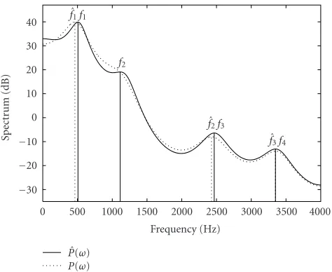
Figure1: AR specturms with and without quantization.
and then define a vector of the peak frequencies as f = (f1,f2,. . .). We here use the peak-picking (PP) method or the
Jenkins-Traub (JT) method to compute f froma.
The PP method finds local maxima of P(ω) by sam-pling it with a constant samsam-pling interval. We applied the PP method with a sampling interval of 1 [Hz] to a set of real speech signals. Then we have f = (507, 1114, 2467, 3349) (Hz). Next we quantized the AR coefficient by using a quan-tizer withα=6. Then we have f =(462, 2429, 3349) (Hz).
Figure 1shows the AR spectrums, where the solid line de-notes the true AR spectrum and the dashed line dede-notes the AR spectrum obtained with the quantized AR coefficients. We see that the second peak labeled “f2” has disappeared due
to rounding errors of the AR coefficients. This phenomenon often occurs in a dull peak such as f2.
The JT method finds the roots of the AR polynomial equation A(z) = 0. The resonance frequency fp and the
bandwidth Bp are then computed from the roots by
us-ing (5) and (6), respectively. As Bp is smaller, the
corre-sponding peak at frequency fpbecomes sharper. Therefore,
in the JT method, we can easily find sharp peaks accord-ing to the bandwidth. Therefore, the peak selection method is effective in overcoming the problem of peak disappear-ance.
3.1.3. Database construction
We putρand f as key and data (nonkey), respectively, and enter a record consisting of key and data items into a database at each time step. Thekd trie (k-dimensional digital search tree) is used as the data structure to allow efficient range searching [26,27]. The average computation time for range searching is onlyO(logN), whereNis the number of records contained in the database. When the database has contained a record with a key equal to the current key, the current record is discarded without being entered into the database.
3.2. Peak frequency estimation using test data
When evaluating the estimation performance, we used a dif-ferent set of speech signals from the ones used for database construction. We recursively computeρnpfromxnby the LSL
algorithm to adapt to changing statistics of signals. We then obtain a coefficient vectorρby quantizingρnpin the same way
as inSection 3.1. We chooseρas a query, and retrieve a co-efficient vector nearest toρ, defined byρ, from the database by range search. More concretely, we retrieve records with keys lying in the space{(ρ1,ρ2,. . .,ρp)| |ρp−ρp| ≤d,∀p}
from the database, wheredis the range size, and increase the value ofd from 0 by one until more than or equal to one record is retrieved. When more than one record is retrieved, the nearest neighbor to the queryρis selected out of them and the corresponding data value (peak frequency) is used as the estimation. In this way, we can recursively estimate peak frequencies without solvingA(z)=0 nor samplingP(ω).
3.3. Experimental results
A speech signal of L seconds from a male is sampled at 8 [kHz] to obtain 8000L records. We then constructed the database consisting of 8000Lrecords. Throughout the sim-ulations, we putλ=0.995 in the LSL algorithm so that good performance is achieved. We evaluated the estimation per-formance by using ten sets of speech signals of one second.
We denote the peak frequency estimation method that directly computes f fromaby using the PP and JT meth-ods as PP1 and JT1, respectively. Algorithm 2 summarizes the JT1 and PP1 methods without using a database. We de-note the proposed estimation method that uses the PP and JT methods to compute f fromaas PP2 and JT2, respec-tively. Algorithm 3 summarizes the JT2 and PP2 methods with using a database. We can estimate degradation of es-timation accuracy due to rounding errors of PARCOR coeffi -cients by comparing the results of the PP1 (JT1) method and PP2 (JT2) method.
We generated several databases by puttingα=5, 6, 7 [bit] and changingLfrom 10 [s] to 500 [s], and measured the es-timation accuracies of the PP2 and JT2 methods. Figures2
and3show the results of the PP2 and JT2 methods, respec-tively. We can measure the estimation accuracy of the PP2 and JT2 methods by the difference between ˆfkandfk, where
fkis the peak frequency estimated by the PP1 (JT1) method
and ˆfk is the one by the PP2 (JT2) method. Spectrum
dis-tortion caused by rounding errors of high order coefficients is relatively small. We thus evaluated the estimation accuracy by checking whether the relative error|fˆk−fk|/ fk<0.1 is sat-isfied or not. When using the JT2 method, we selected sharp peaks of bandwidth less than 500 [Hz]. In both methods, bet-ter results are obtained by puttingα= 6 andL= 500, and the PP2 and JT2 methods achieve accuracies of 78.8% and 76.8%, respectively. The estimation accuracy seems to be im-proved asLis larger.
Peak frequency estimation
(a) Estimateρfromxnby the LSL algorithm.
(b) Transformρintoa.
(c) Compute fcorresponding toawith the PP (JT) method.
(d) Go to step (a).
Algorithm2: JT1 (PP1) method.
Database construction using training data (a) Estimateρfromxnby the LSL algorithm.
(b) Quantizeρintoρ, and then transform
ρintoa.
(c) Computef corresponding toawith the PP (JT) method.
(d) Enter (ρ, f) into a database. (e) Go to step (a).
Peak frequency estimation using test data (a) Estimateρfromxnby the LSL algorithm.
(b) Quantizeρintoρ.
(c) Findρby range search, where the range size is increased by one until more than or equal to one record is retrieved. (d) Choosef corresponding toρas the
estimation. (e) Go to step (a).
Algorithm3: JT2 (PP2) method.
same. We can explain the reason as follows: if a record of (ρ,f) is stored for each bin distributed inρ-space, a finer quantization of PARCOR coefficients results in a higher esti-mation accuracy. However, the database size would become extremely large, because the number of bins is increased by a factor of 2Pasαis increased by one. The estimation accuracy
improves with an increase of the number of records, only un-der the assumption that we store a record for each bin. When the assumption is not satisfied, as is the current case, the im-provement is not expected.
As mentioned earlier, the current record is discarded when a record with a key equal to the current key has been stored in the database. We thus evaluated the number of records in the database, the rate to the total number of records, and the storage space.Table 1summarizes the results forL=500. We see that the database size forα=7 is large enough, and the number of records stored in the database increases asαis larger.
Figures4aand4bplot peak frequencies for every 50 time steps estimated by the JT1 and JT2 methods. We putL=500 andα=6 in the JT2 method, because this choice gave good result as shown in Figures2and3. We see that the results of the JT1 and JT2 methods are very close to each other, but differ in some snapshots.
Finally we measured the computation time of the PP1, PP2, JT1, and JT2 methods on a personal computer with an Intel Pentium III 1 GHz. Most of the computation time is spent in range searching in the PP2 and JT2 methods, and peak finding in the PP1 and JT1 methods. In other words,
Time (s)
Estimatio
n
ac
curacy
(%)
50 60 70 80
0 100 200 300 400 500
α=5 α=6 α=7
Figure2: Estimation accuracy of PP2 for different values ofLandα.
Time (s)
Estimatio
n
ac
curacy
(%)
50 60 70 80
0 100 200 300 400 500
α=5 α=6 α=7
Figure3: Estimation accuracy of JT2 for different values ofLandα.
the computational complexities of the LSL algorithm and (8) are negligibly small as compared to range searching and peak finding. The computation times of the PP1, JT1, and JT2 (PP2) methods required for processing signals of one second are 84.0 seconds, 5.3 seconds, and 5.0 seconds, respectively. The JT2 (PP2) method is much faster than the PP1 method, but the computation time is almost the same as that of the JT1 method, and real-time processing is not possible in ei-ther case.
4. IMPROVED ESTIMATION METHOD
4.1. Simultaneous execution of database construction and estimation
Table1: Number of records in the database for different values ofα.
α(bit) 5 6 7
Number of records 1.9×10
5 5.8×10⁵ 1.2×10⁶
(4.7%) (14.5%) (29.2%)
Storage space (MB) 61 108 170
Time (s)
Fre
q
u
en
cy
(H
z)
0 500 1000 1500 2000 2500 3000 3500 4000
0 0.5 1
(a)
Time (s)
Fre
q
u
en
cy
(H
z)
0 500 1000 1500 2000 2500 3000 3500 4000
0 0.5 1
(b) Figure4: Plots of peak frequencies: (a) JT1 and (b) JT2.
due to the fact that searching in the large database of size 108 (MB) is computationally expensive, and that the range size is repeatedly increased by one until more than or equal to one record is retrieved. The repeated range search in-creases the processing time, and degrades the estimation accuracy with an increase of range size, because records with keys far apart from a query are extracted from the database.
The estimation accuracies of the PP2 and JT2 meth-ods strongly depend on the database contents, for example, whether training and test data are from the same speaker or not, whether acoustic environments in training and testing phases are the same or not. We have to build a large database if we would store a large number of records obtained from different speakers in different acoustic environments. How-ever, searching in the large database requires large compu-tation time and memory requirements. As can be seen from
Table 1, the database size is large enough even when we store speech signals from only one speaker. A further data inser-tion into the database should be avoided from the view point of processing speed and storage space.
For the solution, we simultaneously execute database construction and peak frequency estimation. We first set the maximum range size as dmax so that records with keys far
apart from a query are not retrieved. We then compute the peak frequency vector f associated with the current PAR-COR coefficient ρ by using the JT method, only when no record is retrieved by range search withd=dmax, we choose
f as the estimation, and then enter a record of (f,ρ) into the
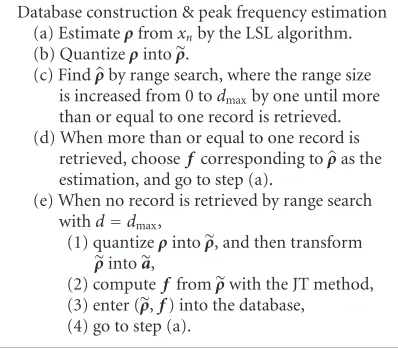
Database construction & peak frequency estimation (a) Estimateρfromxnby the LSL algorithm.
(b) Quantizeρintoρ.
(c) Findρby range search, where the range size is increased from 0 todmaxby one until more than or equal to one record is retrieved. (d) When more than or equal to one record is
retrieved, choosef corresponding toρas the estimation, and go to step (a).
(e) When no record is retrieved by range search withd=dmax,
(1) quantizeρintoρ, and then transform
ρintoa,
(2) computef fromρwith the JT method, (3) enter (ρ,f) into the database, (4) go to step (a).
Algorithm4: JT3 method.
database. The simultaneous execution technique decreases processing time and increases estimation accuracy by appro-priately choosingdmax. We here denote the improved
Table2: Estimation accuracy and processing time forα=6.
dmax 0 1 2 3
Number of records 11655 9665 2261 2212
(14.5%) (12.1%) (2.8%) (2.8%)
Accuracy 91.2% 91.0% 88.0% 88.0%
Time (s) 1.18 0.97 0.55 0.55
Table3: Estimation accuracy and processing time forα=7.
dmax 0 2 4 6
Number of records 22705 6211 1516 1477
(28.4%) (7.8%) (1.9%) (1.8%)
Accuracy 95.6% 94.6% 89.5% 87.4%
Time (s) 1.81 0.79 0.53 0.53
Table4: Estimation accuracy and processing time forα=8.
dmax 0 4 6 8 12
Number of records 36060 4398 3200 1826 1004
(45.0%) (5.5%) (4.0%) (2.3%) (1.3%)
Accuracy 98.0% 95.4% 95.2% 92.2% 89.1%
Time (s) 2.68 0.70 0.64 0.61 0.63
Table5: Estimation accuracy and processing time forα=9.
dmax 0 8 16 24
Number of records (6249793.2%) (65168.5%) (22048.6%) (11095.4%)
Accuracy 99.0% 96.7% 92.6% 89.4%
Time (s) 3.58 0.81 0.74 0.82
4.2. Experimental results
We have applied the JT3 method to ten sets of speech sig-nals of one second, and have measured the estimation accu-racy of four peak frequencies (f1,f2,f3,f4), the number of
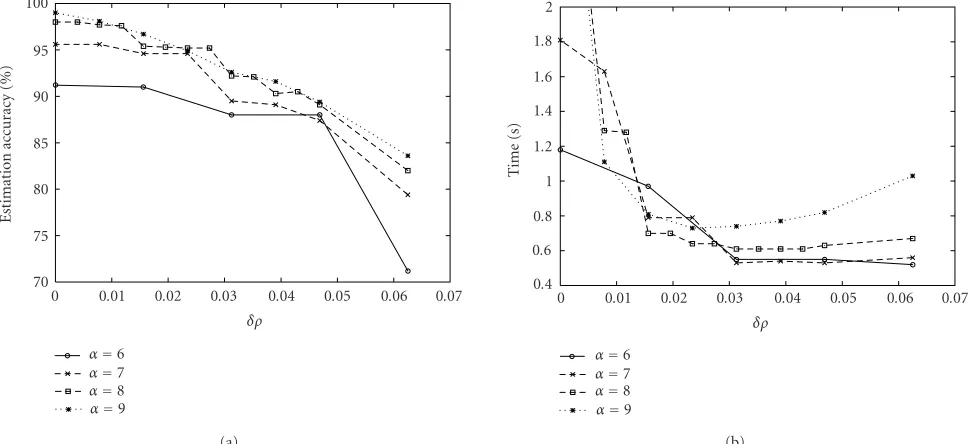
records in database, and the processing time per 8000 sam-ples (one second) for different values ofαanddmax. Tables 2,3,4, and 5summarize the results for α = 6, 7, 8, 9, re-spectively. Since the range size in ρ-space is represented by
δρ =dmax/2α, the actual range sizes for (α = a,dmax = b)
and (α = a+ 1,dmax = 2b) are the same.Figure 5shows
the estimation accuracy and the processing time for different values ofδρ. We see that the database size and the process-ing time decrease asdmaxis larger, while the estimation
ac-curacy decreases. If we putdmax =0 and α = ∞, a perfect
accuracy of 100% is achieved. However, instead of achieving perfect accuracy, the time-consuming polynomial rooting is frequently done. A choice ofα=9 anddmax=0 achieves the
best accuracy of 99.0%, but requires a large processing time of 3.58 seconds. A choice of α = 6 anddmax = 4 achieves
the fastest processing speed of 0.52 second, but provides poor
accuracy of 71.2%. We have to make a tradeoffbetween pro-cessing time and estimation accuracy in choosingαanddmax.
When the sampling interval is large, we can makeαlarge and
dmax small to improve estimation accuracy. When the
sam-pling interval is small, we should makeαsmall anddmaxsmall
to reduce processing time. The optimal choice depends on the application. In the current application, 8000 sample data must be processed within one second. Therefore, we should putα=8 anddmax =6, because this choice gave a
satisfac-tory accuracy of 95.2% with a processing time of 0.64 second per 8000 samples.Figure 6plots the estimated peak frequen-cies. It is evident that the estimation result is better than the previous one inFigure 4b.
4.3. Database update procedure
In the JT3 method, the current record is entered into the database when no record is retrieved by range search with
d = dmax. Therefore, the database size monotonously
δρ
Estimatio
n
ac
curacy
(%)
70 75 80 85 90 95 100
0 0.01 0.02 0.03 0.04 0.05 0.06 0.07
α=6 α=7 α=8 α=9
(a)
δρ
Ti
m
e
(s
)
0.4 0.6 0.8 1 1.2 1.4 1.6 1.8 2
0 0.01 0.02 0.03 0.04 0.05 0.06 0.07
α=6 α=7 α=8 α=9
(b)
Figure5: Results of the improved estimation method: (a) estimation accuracy and (b) processing time.
Time (s)
Fre
q
u
en
cy
(H
z)
0 500 1000 1500 2000 2500 3000 3500 4000
0 0.5 1
Figure6: Plots of peak frequencies obtained by JT3.
We thus update the database contents according to times-tamp. More precisely, we determined the maximum num-ber of records in the database asNmax, and deleted the
old-est record from the database if the number of records in the database exceedsNmax. The oldest record in thekd trie can
be easily deleted without adding the time index into the key field [28].
Table 4shows that the number of records is about 3200 when we putα=8 anddmax=6. We thus putNmax=4000,
and measured the processing time per 8000 samples.Figure 7
plots the result using speech signals of 500 seconds, where the solid and dashed lines denote the results with and with-out database update, respectively. We see that the processing time of the JT3 method without database update becomes larger as time passes, while the processing time with database update is almost constant, because the maximum number of records in the database is fixed at 4000. The estimation
ac-Time (s)
P
roc
essing
time
(s)
100 200 300 400 500
0.5 0.6 0.7 0.8 0.9 1.0 1.1
With update Without update
Figure7: Processing time with and without database update (single speaker).
curacies with and without database update are 92.7% and 92.3%, respectively. They are found to be almost the same. We see that the database update procedure can make the pro-cessing time almost constant with maintaining high estima-tion accuracy.
Time (s)
P
roc
essing
time
(s)
100 200 300 400 500
0.5 0.6 0.7 0.8 0.9 1.0 1.1
With update Without update
Figure8: Processing time with and without database update (mul-tiple speakers).
4.4. Application to LSP estimation
Also LSP (line spectrum pair) can be uniquely characterized by the PARCOR coefficients, and polynomial root finding is required to compute LSPs from PARCOR coefficients. We thus replaced peak frequencies by LSPs in the key field, and estimated LSPs by using the JT3 method with database up-date. Figure 9b plots the estimated LSPs for every 50 time steps, where we put p = 10 andα = 6. The result of the JT1 method is shown inFigure 9afor comparison purpose. The processing times of the JT1 and JT3 methods per 8000 samples are 9.2 seconds and 0.96 second, respectively, and the JT3 method achieves a very good accuracy of 98.4%.
5. CONCLUSION
We have developed the fast and recursive peak frequency es-timation method using a database of PARCOR coefficients. We have investigated searching range size and quantization interval of PARCOR coefficients so that a good tradeoff be-tween estimation accuracy and processing speed is achieved. We have simultaneously executed database construction and peak frequency estimation for decreasing processing time and increasing estimation accuracy. Moreover, we have up-dated the database contents according to timestamp so that processing time is not monotonously increased. We have also applied the database-based method to LSP estimation, and have shown the effectiveness.
The concept of the database-based method originally comes from an intelligent landing system designed previ-ously by one of authors [29]. It is very difficult to model a human skill with a simple mathematical equation. We thus built a database that stores aircraft states as key and con-trol commands provided by a human expert as nonkey, and succeeded to generate a control command close to human operation by database searching. The PARCOR coefficient and the peak frequency presented in this paper correspond to the aircraft state and the control command, respectively.
Time (s)
Fre
q
u
en
cy
(H
z)
0 500 1000 1500 2000 2500 3000 3500 4000
0 0.5 1
(a)
Time (s)
Fre
q
u
en
cy
(H
z)
0 500 1000 1500 2000 2500 3000 3500 4000
0 0.5 1
(b)
Figure9: Plots of LSPs: (a) JT1 and (b) JT3.
REFERENCES
[1] D. H. Johnson, “The application of spectral estimation meth-ods to bearing estimation problems,” Proc. IEEE, vol. 70, no. 9, pp. 1018–1028, 1982.
[2] G. Parati, J. P. Saul, D. M. Rienzo, and G. Mancia, “Spectral analysis of blood pressure and heart rate variability in evalu-ating cardiovascular regulation: A critical appraisal.,” Hyper-tension, vol. 25, no. 6, pp. 1276–1286, 1995.
[3] D. W. Rickey and A. Fenster, “Evaluation of an automated real-time spectral analysis technique,”Ultrasound in Medicine and Biology, vol. 22, no. 1, pp. 61–73, 1996.
[4] M. Arnold, H. Witte, P. Leger, H. Boccalon, S. Bertuglia, and A. Colantuoni, “Time-variant spectral analysis of LDF signals on the basis of multivariate autoregressive modelling,” Tech-nology and Health Care, vol. 7, no. 2–3, pp. 103–112, 1999. [5] I. G¨ulera, M. K. Kiymikb, M. Akinc, and A. Alkan, “AR
spec-tral analysis of EEG signals by using maximum likelihood es-timation,” Computers in Biology and Medicine, vol. 31, pp. 441–450, 2001.
[7] J. Markel, “Digital inverse filtering-a new tool for formant trajectory estimation,” IEEE Transactions on Audio and Elec-troacoustics, vol. 20, no. 2, pp. 129–137, 1972.
[8] S. S. McCandless, “An algorithm for automatic formant ex-traction using linear prediction spectra,” IEEE Trans. Acous-tics, Speech, and Signal Processing, vol. 22, no. 2, pp. 135–141, 1974.
[9] N. Ouaaline and L. Radouane, “Pole zero estimation of speech signal based on zero tracking algorithm,” Advances in Mod-elling & Analysis B, vol. 30, no. 4, pp. 35–48, 1994.
[10] A. Alwan, “Modeling speech production and perception mechanisms and their applications to synthesis, recognition, and coding,” inProc. IEEE 5th International Symposium on Signal Processing and Its Applications (ISSPA ’99), vol. 1, p. 7, Brisbane, Queensland, Australia, 1999.
[11] D. W. Guillaume, “A comparison of peak frequency-time plots produced with Hilbert and wavelet transforms,” Review of Scientific Instruments, vol. 73, no. 1, pp. 98–101, 2002. [12] P. F. Assmann and W. F. Katz, “Time-varying spectral change
in the vowels of children and adults,”Journal of the Acoustical Society of America, vol. 108, no. 4, pp. 1856–1866, 2000. [13] I. Bazzi, A. Acero, and L. Deng, “An
expectation-maximization approach for formant tracking using a parameter-free non-linear predictor,” inProc. IEEE Interna-tional Conference on Acoustics, Speech, and Signal Processing (ICASSP ’03), vol. 1, pp. 464–467, Hong Kong, 2003. [14] S. M. Kay and S. L. Marple Jr., “Spectrum analysis: A modern
perspective,”Proc. IEEE, vol. 69, no. 11, pp. 1380–1419, 1981. [15] D. Hush, N. Ahmed, and R. David, “Instantaneous frequency estimation using adaptive linear predictor weights,” IEEE Trans. on Aerospace and Electronics Systems, vol. AES-22, no. 4, pp. 442–431, 1986.
[16] T. J. Shan and T. Kailath, “Directional signal separation by adaptive arrays with a root-tracking algorithm,” inProc. Inter-national Conference on Acoustics, Speech, and Signal Processing (ICASSP ’87), pp. 2288–2291, Dallas, TX, USA, 1987. [17] S. Orfanidis and L. Vail, “Zero-tracking adaptive filters,”IEEE
Transactions on Acoustics, Speech, and Signal Processing, vol. 34, no. 6, pp. 1566–1572, 1986.
[18] A. Nehorai and D. Starer, “Adaptive pole estimation,” IEEE Transactions on Acoustics, Speech, and Signal Processing, vol. 38, no. 5, pp. 825–838, 1990.
[19] L. Jackson and S. Wood, “Linear prediction in cascade form,” IEEE Transactions on Acoustics, Speech, and Signal Processing, vol. 26, no. 6, pp. 518–528, 1978.
[20] P. C. Chin, C. C. Goodyear, and D. Phil, “Adaptive cascade filter for speech analysis,”IEE Proc., vol. 130, no. 1, pp. 11–18, 1983.
[21] G. Rigoll, “A new algorithm for estimation of formant tra-jectories directly from the speech signal based on an ex-tended Kalman-filter,” inProc. IEEE International Conference on Acoustics, Speech, and Signal Processing, (ICASSP ’86), pp. 1229–1232, Tokyo, 1986.
[22] J. Makhoul, “Linear prediction: A tutorial review,”Proc. IEEE, vol. 63, no. 4, pp. 561–580, 1975.
[23] B. Farhang-Boroujeny, Adaptive Filters: Theory and Applica-tions, Wiley & Sons, New York, NY, USA, 1998.
[24] N. Kitawaki and F. Itakura, “Efficient coding of speech by nonlinear quantization and nonuniform sampling of PAR-COR coefficients,” Transactions of the Institute of Electronics and Communication Engineers of Japan (IEICE), vol. J61-A, no. 6, pp. 543–550, 1978.
[25] N. Kitawaki, F. Itakura, and S. Saito, “Optimum coding of transmission parameters in PARCOR speech analysis synthe-sis system,,” Transactions of the Institute of Electronics and Communication Engineers of Japan (IEICE), vol. J61-A, no. 2, pp. 119–126, 1978.
[26] E. Fredkin, “Trie memory,” Comm. ACM, vol. 3, no. 9, pp. 490–499, 1960.
[27] J. A. Orenstein, “Multidimensional tries used for associative searching,”Inf. Process. Lett., vol. 14, no. 4, pp. 150–157, 1982. [28] Y. Iiguni, I. Kawamoto, and N. Adachi, “A nonlinear adap-tive estimation method based on local approximation,”IEEE Trans. Signal Processing, vol. 45, no. 7, pp. 1831–1841, 1997. [29] Y. Iiguni, H. Akiyoshi, and N. Adachi, “An intelligent landing
system based on a human skill model,” IEEE Trans. Aerosp. Electron. Syst., vol. 34, no. 3, pp. 877–882, 1998.
Tetsuya Watanabe received his B.E. and M.E. degrees in communications engineer-ing from Osaka University, Osaka, Japan, in 2001 and 2003, respectively. Since 2003, he has been working in Frontier Systems Group Network Division, NEC TOSHIBA Space Systems, Ltd., Yokohama, Japan.