Volume 2006, Article ID 71459, Pages1–14 DOI 10.1155/ASP/2006/71459
A Frequency Domain Approach to Registration of
Aliased Images with Application to Super-resolution
Patrick Vandewalle,1Sabine S ¨usstrunk,1and Martin Vetterli1, 2
1Ecole Polytechnique F´ed´eral de Lausanne, School of Computer and Communication Sciences, 1015 Lausanne, Switzerland 2Department of Electrical Engineering and Computer Sciences, University of California, Berkeley, CA 94720-1770, USA
Received 27 November 2004; Revised 4 May 2005; Accepted 18 May 2005
Super-resolution algorithms reconstruct a high-resolution image from a set of low-resolution images of a scene. Precise alignment of the input images is an essential part of such algorithms. If the low-resolution images are undersampled and have aliasing artifacts, the performance of standard registration algorithms decreases. We propose a frequency domain technique to precisely register a set of aliased images, based on their low-frequency, aliasing-free part. A high-resolution image is then reconstructed using cubic interpolation. Our algorithm is compared to other algorithms in simulations and practical experiments using real aliased images. Both show very good visual results and prove the attractivity of our approach in the case of aliased input images. A possible application is to digital cameras where a set of rapidly acquired images can be used to recover a higher-resolution final image.
Copyright © 2006 Patrick Vandewalle et al. This is an open access article distributed under the Creative Commons Attribution License, which permits unrestricted use, distribution, and reproduction in any medium, provided the original work is properly cited.
1. INTRODUCTION
Image resolutionis one of the limitingparameters in digital camera design. With most digital cameras, however, it is pos-sible to take bursts of multiple pictures in a very short period of time. Thus, high-resolution images can be reconstructed from a series of low-resolution images using super-resolution algorithms.
The idea behind super-resolution imaging is to combine the information from a set of slightly different low-resolution images of the same scene and use it to construct a higher-resolution image. Throughout this paper, a higher-higher-resolution image is defined as an image with more resolving power. This means that an image that is obtained by merely upsampling and interpolating a low-resolution image does not have a higher resolution than its original. It has a larger number of pixels, but the resolving power remains the same; that is, the interpolated image does not contain more details than its original. The resolving power of an image can be increased by adding high-frequency information typically based on knowledge about the specific image model. A higher resolv-ing power is also obtained when the aliasresolv-ing ambiguity in an image is removed. We will take this second approach to construct high-resolution images. The aliasing ambiguity in an image is removed by incorporating the additional infor-mation obtained from other images of the same scene.
We describe an image registration algorithm using a new frequency domain method that outperforms the state of the art in frequency domain registration methods. It also performs better than the spatial domain method by Keren et al. [5] if the images have some directionality. Unlike other motion estimation algorithms whose performance is often very low for noisy or highly aliased images (seeSection 2), our algorithm only uses low-frequency information. This is the part of the signals with the highest signal-to-noise ratio (SNR), and in our setup, the aliasing-free part of the images. We developed a new, computationally efficient method to es-timate planar rotations. To reconstruct the high-resolution image, we apply bicubic interpolation on a high-resolution grid. The super-resolution algorithm we propose recon-structs an image with almost double resolution in both di-mensions from four aliased images. The four low-resolution images are necessarily undersampled. Otherwise, our algo-rithm is not able to reconstruct a better image as it uses ex-actly this undersampled information. We compare our ap-proach in a simulation to other spatial domain and frequency domain registration algorithms. We find that our algorithm can better estimate shift and rotation parameters than the other methods, in particular, when some strong direction-ality is present in the image.
A possible application of the proposed image registra-tion algorithm is that of a user holding his digital camera in his hands while manually or automatically taking a se-ries of four shots of a scene within a short period of time. The small vibrations of the user’s hands during image cap-ture are sufficient to reconstruct a high-resolution image. The scene needs to be flat or at a large distance, such that no parallax effects take place. We tested such a setup us-ing real digital cameras. We verified that aliasus-ing occurs with these cameras by measuring their spatial frequency response. In the experiments, we found that our algorithm results in better visual quality than the other methods, which typically failed to adequately register all four images. Other applica-tions of super-resolution algorithms can be found in foren-sic imaging, satellite imaging, microscopy, medical imaging, constructing still images from video sequences, and so forth. The article is organized as follows.Section 2discusses the state of the art in image registration and super-resolution imaging. The planar motion estimation algorithm is de-scribed in Section 3 and the reconstruction in Section 4.
Section 5shows the results on simulated and real images and the comparison to other algorithms. The results are discussed in Sections6and7concluding the article.
2. STATE OF THE ART
The idea of super-resolution was first introduced in 1984 by Tsai and Huang [1] for multiframe image restoration of ban-dlimited signals. A good overview of existing algorithms is given by Borman and Stevenson [14] and Park et al. [15]. Most super-resolution methods are composed of two main steps: first all the images are aligned in the same coordinate system in the registration step, and then a high-resolution image is reconstructed from the irregular set of samples. In
this second step, the camera point spread function is often taken into account.
Precise subpixel image registration is a basic requirement for a good reconstruction. If the images are inaccurately reg-istered, the high-resolution image is reconstructed from in-correct data and is not a good representation of the orig-inal signal. Zitov´a and Flusser [16] presentan overview of image registration methods. Registration can be done ei-ther in spatial or in frequency domain. By the nature of the Fourier transform, frequency domain methods are limited to global motion models. In general, they also consider only planar shifts and possibly planar rotation and scale, which can be easily expressed in Fourier domain. However, aliasing is much easier to describe and to handle in frequency domain than in spatial domain.
Tsai and Huang [1] describe an algorithm to register mul-tiple frames simultaneously using nonlinear minimization in frequency domain. Their method for registering multiple aliased images is based on the fact that the original, high-resolution signal is bandlimited. It is not clear, however, if such a solution is unique and if such an algorithm will not converge to a local minimum. Most of the frequency do-main registration methods are based on the fact that two shifted images differ in frequency domain by a phase shift only, which can be found from their correlation. Using a log-polar transform of the magnitude of the frequency spectra, image rotation and scale can be converted into horizontal and vertical shifts. These can therefore also be estimated us-ing a phase correlation method. Reddy and Chatterji [17] and Marcel et al. [18] describe such planar motion estimation al-gorithms. Reddy and Chatterji apply a high-pass emphasis filter to strengthen high frequencies in the estimation. Kim and Su [19], Stone et al. [20], and Vandewalle et al. [2] also apply a phase correlation technique to estimate planar shifts. To minimize errors due to aliasing, their methods rely on a part of the frequency spectrum that is almost free of alias-ing. Typically this is the low-frequency part of the images. Foroosh et al. [21] showed that the signal power in the phase correlation corresponds to a polyphase transform of a filtered unit impulse. Lucchese and Cortelazzo [22] developed a ro-tation estimation algorithm based on the property that the magnitude of the Fourier transform of an image and the mir-rored version of the magnitude of the Fourier transform of a rotated image have a pair of orthogonal zero-crossing lines. The angle that these lines make with the axes is equal to half the rotation angle between the two images. The horizontal and vertical shifts are estimated afterwards using a standard phase correlation method.
motion models, such as affine flow or rigid body motion, can be used in combination with this approach. Irani et al. [25] present a method to compute multiple, possibly transparent or occluding motions in an image sequence. Motion is esti-mated using an iterative multiresolution approach based on planar motion. Different objects are tracked using segmen-tation and temporal integration. Gluckman [26] describes a method that first computes planar rotation from the gradient field distribution of the images to be registered. Planar shifts are then estimated after cancellation of the rotation using a phase correlation method.
In the subsequent image reconstruction phase, a high-resolution image is reconstructed from the irregular set of samples that is obtained from the different low-resolution images. This can be achieved using an interpolation-based method as the one used by Keren et al. [5]. Tsai and Huang [1] describe a frequency domain method, writing the Fourier coefficients of the high-resolution image as a function of the Fourier coefficients of the registered low-resolution images. The solution is then computed from a set of linear equations. This algorithm uses the same principle as the formulation in time domain given by Papoulis [27]. A high-resolution image can also be reconstructed using a POCS algorithm (Patti et al. [10]), where the estimated reconstruction is suc-cessively projected on different convex sets. Each set repre-sents constraints to the reconstructed image that are based on the given measurements and assumptions about the sig-nal. Capel and Zisserman [4] and Schultz et al. [6] use a maximum a posteriori (MAP) statistical method to build the high-resolution image.
Other methods iteratively create a set of low-resolution images from the estimated image using the imaging model. The estimate is then updated according to the difference between the real and the simulated low-resolution images (Keren et al. [5], Irani and Peleg [7]). This method is known as iterative backprojection. Zomet et al. [11] improved the results obtained with typical iterative backprojection algo-rithms by taking the median of the errors in the different backprojected images. This proved to be more robust in the presence of outliers. Farsiu et al. [12] proposed a new and robust super-resolution algorithm. Instead of the more com-monL2minimization, they use theL1norm, which produces sharper high-resolution images. They also showed that this approach performs very well in combination with the al-gorithm by Zomet et al. [11]. Elad and Feuer [13] present a super-resolution framework that combines a maximum-likelihood/MAP approach with a POCS approach to define a new convex optimization problem. Next, they show the con-nections between their method and different classes of other existing methods.
Our main contribution in this paper consists of a new frequency domain algorithm to register not just low resolu-tion, but also aliased images. We use a planar motion model. When a series of images is taken in a short amount of time with only small camera motion between the images, we as-sume that the motion can be described with such a model. In general, a planar model is simpler and has less parame-ters making it often more robust in the presence of noise. We
also extend the planar shift motion model from [2,19,20] to include planar rotations, because they are often part of the camera motion. Even a small rotation has a large influence on final registration. Our rotation estimation algorithm is com-putationally efficient and adapted to work with aliased im-ages. We test our algorithm not only in simulations, but also on real sequences of aliased images. The results from these tests validate the assumptions made about the motion. They show, both visually and in SNR, that our algorithm outper-forms other frequency domain registration methods as well as a spatial domain method if directionality is present in the images.
3. PLANAR MOTION ESTIMATION
We use a frequency domain algorithm to estimate the mo-tion parameters between the reference image and each of the other images. Only planar motion parallel to the image plane is allowed. The motion can be described as a function of three parameters: horizontal and vertical shifts,Δx1andΔx2, and a planar rotation angleφ.
A frequency domain approach allows us to estimate the horizontal and vertical shift and the (planar) rotation sepa-rately. Assume we have a reference signal f1(x) and its shifted and rotated version f2(x):
f2(x)= f1
R(x+Δx),
withx=
x1
x2
, Δx=
Δx1 Δx2
, R=
cosφ −sinφ
sinφ cosφ
.
(1)
This can be expressed in Fourier domain as
F2(u)=
x f2(x)e
−j2πuTx
dx
=
x f1
R(x+Δx)e−j2πuTxdx
=ej2πuTΔx
x f1(Rx
)e−j2πuTx
dx,
(2)
withF2(u) the Fourier transform off2(x) and the coordinate transformationx = x+Δx. After another transformation x=Rx, the relation between the amplitudes of the Fourier
transforms can be computed as
F2(u)=ej2πuTΔx
x f1(Rx
)e−j2πuTx
dx
=
x f1(Rx
)e−j2πuTx
dx
=
x f1(x
)e−j2πuT(RTx)
dx
=
x f1(x
)e−j2π(Ru)Tx
dx
=F1(Ru),
(a) (b)
−100 −80 −60 −40 −20 0 20 40 60 80 100 Angleα(degrees)
0 0.5 1 1.5 2 2.5 3 3.5×10
4
h
(
α
)
Original image Rotated image
(c)
Figure1: Rotation estimation. (a) Frequency values of the reference image for 0.1ρ < r < ρ. (b) Frequency values of the rotated image (φ=25 degrees) for 0.1ρ < r < ρ. (c) Average value as a function of the angleh(α) for both|F1(u)|and|F2(u)|.
where|F2(u)|is a rotated version of|F1(u)|over the same angleφas the spatial domain rotation (see Figures1(a)and
1(b)).|F1(u)|and|F2(u)|do not depend on the shift values Δx, because the spatial domain shifts only affect the phase values of the Fourier transforms. Therefore we can first esti-mate the rotation angleφfrom the amplitudes of the Fourier transforms|F1(u)|and|F2(u)|. After compensation for the rotation, the shiftΔxcan be computed from the phase diff er-ence betweenF1(u) andF2(u).
InSection 3.1, we give a precise rotation estimation al-gorithm. A subpixel shift estimation algorithm is described inSection 3.2, and an adaptation of this method to estimate motion accurately in aliased images is presented inSection 3.3.
3.1. Rotation estimation
The rotation angle between|F1(u)|and|F2(u)|can be com-puted as the angleθfor which the Fourier transform of the reference image|F1(u)|and the rotated Fourier transform of the image to be registered|F2(Rθu)|have maximum correla-tion. This implies the computation of a rotation of|F2(u)| for every evaluation of the correlation, which is computa-tionally heavy and thus practically difficult.
If|F1(u)|and|F2(u)|are transformed in polar coordi-nates, the rotation over the angleφis reduced to a (circular) shift overφ. We can compute the Fourier transform of the spectra|F1(u)|and|F2(u)|, and computeφas the phase shift between the two (as it was also done by Marcel et al. [18] and Reddy and Chatterji [17]). This requires a transformation of the spectrum to polar coordinates. The data from the regular
x1,x2-grid need to be interpolated to obtain a regularr,θ -grid. Mainly for the low frequencies, which generally contain most of the energy, the interpolations are based on very few
function values and thus introduce large approximation er-rors. An implementation of this method is also computation-ally intensive.
Our approach is computationally much more efficient than the two methods described above. First of all, we com-pute the frequency contenthas a function of the angleαby integrating over radial lines:
h(α)= α+Δα/2
α−Δα/2 ∞
0
F(r,θ)dr dθ. (4)
In practice,|F(r,θ)|is a discrete signal. Therefore, we com-pute the discrete functionh(α) as the average of the values on the rectangular grid that have an angleα−Δα/2 < θ < α+Δα/2. As we want to compute the rotation angle with a precision of 0.1 degrees, h(α) is computed every 0.1 de-grees. To get a similar number of signal values |F(r,θ)|at every angle, the average is only evaluated on a circular disc of values for which r < ρ (whereρ is the image radius or half the image size). Finally, as the values for low frequen-cies are very large compared to the other values and are very coarsely sampled as a function of the angle, we discard the values for whichr < ρ, with =0.1. Thus,h(α) is com-puted as the average of the frequency values on a discrete grid withα−Δα/2< θ < α+Δα/2 andρ < r < ρ.
umaxu
F(u)
0 0.2 0.4 0.6 0.8 1 Timet −8 −6 −4 −2 0 2 4 6 8 f ( t ) (a)
us−umaxuus max u
F(u)
0 0.2 0.4 0.6 0.8 1 Timet −8 −6 −4 −2 0 2 4 6 8 f ( t ) (b)
us−umax us
umax u
F(u)
0 0.2 0.4 0.6 0.8 1 Timet
−1
−0.8
−0.6
−0.4
−0.20 0.2 0.4 0.6 0.18
f
(
t
)
(c)
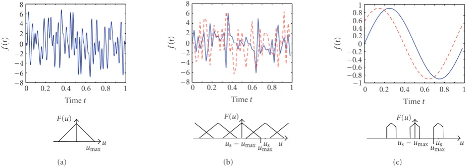
Figure2: In the presence of (partial) aliasing, the shift between two sampled signals cannot be found directly. However, after low-pass filtering, the shift can be easily determined. (a) Original continuous-time signal in time and frequency domain. (b) Sampled signal in time and frequency domain, with aliasing. (c) Low-pass filtered sampled signal in time and frequency domain.
3.2. Shift estimation
A shift of the image parallel to the image plane can be ex-pressed in Fourier domain as a linear phase shift:
F2(u)=
x f2(x)e
−j2πuTx
dx=
xf1(x+Δx)e
−j2πuTx
dx
=ej2πuTΔx
x f1(x
)e−j2πuTx
dx=ej2πuTΔxF1(u).
(5)
It is well known that the shift parameters Δx can thus be computed as the slope of the phase difference ∠(F2(u)/ F1(u)). To make the solution less sensitive to noise, a plane is fitted through the phase differences using a least squares method.
3.3. Aliasing
If the low-resolution images are aliased, the methods de-scribed earlier do not result in precise registration anymore. This is due to the difference in frequency content of the low-resolution images caused by the aliasing. In this case, (2), (3), and (5) no longer hold. Instead of (5), a shift is now expressed as
F2(u)= K
k=−K
ej2π(u−kus)TΔxF 1
u−kus
, (6)
withusthe sampling frequency and 2K+ 1 overlapping spec-trum copies at frequencyu. Aliasing terms disturb the linear phase relation betweenF1(u) andF2(u). However, in cases of limited aliasing, it is still possible to use the above methods, by considering only the frequencies that are free of aliasing or only marginally affected by aliasing. A similar idea was used for shift estimation methods by Kim and Su [19] and by Stone et al. [20].
Assume a one-dimensional, bandlimited signal f(x) (with maximum frequencyumax,Figure 2(a)), which is sam-pled at a frequencyumax < us<2umax. This does not satisfy the Nyquist criterion, and the sampled signal f[k] will have aliasing artifacts (Figure 2(b)). f(x) cannot be perfectly re-constructed from the samples f[k]. Consider two sampled signals, f1[k] and f2[k], sampled at 0,T, 2T,. . .,kT,. . .and Δx,T+Δx, 2T+Δx,. . .,kT+Δx,. . ., respectively (withT= 1/usthe sampling period). Due to the aliasing, their Fourier transforms differ by more than just a linear phase shift, and the shift estimation method described above does not work any more. However, the values at frequencies−us+umax <
u < us−umaxare free of aliasing and thus the same for the two sampled signals f1[k] and f2[k] (up to a linear phase shift). So if a low-pass filter is applied to f1[k] and f2[k], the re-sulting signals f1,low[k] and f2,low[k] are exactly the same up to their shiftΔx(Figure 2(c)). This shift can then be derived using a correlation operator in time domain or by estimating the linear phase difference in frequency domain.
An extension to two dimensions is straightforward. The two sampled signals f1[k] and f2[k] are first low-pass fil-tered (with cutoff frequency us−umax) in horizontal and vertical dimensions. The filtered images are identical up to their registration parameters and can be registered using the methods described in Sections3.1 and3.2. As both meth-ods are applied in the Fourier domain, the filtering step can be avoided by applying the registration algorithms imme-diately to the low frequencies. The rotation estimation is then based on the frequencies for which ρ < r < ρmax (withρmax =min((us−umax)/us)), and the horizontal and vertical shifts are estimated from the phase differences for −us+umax<u<us−umax.
(1) Multiply the imagesfLR,mby a Tukey window to make them circularly symmetric. The windowed images are called fLR,w,m.
(2) Compute the Fourier transformsFLR,w,mof all low-resolution images.
(3) Rotation estimation: the rotation angle between every image fLR,w,m(m=2,. . .,M) and the reference imagefLR,w,1is estimated.
(a) Compute the polar coordinates (r,θ) of the image samples.
(b) For every angleα, compute the average valuehm(α) of the Fourier coefficients for whichα−1< θ < α+ 1 and 0.1ρ < r < ρmax.
The angles are expressed in degrees andhm(α) is evaluated every 0.1 degrees. A typical value used forρmaxis 0.6.
(c) Find the maximum of the correlation betweenh1(α) andhm(α) between−30 and 30 degrees. This is the estimated rotation
angleφm.
(d) Rotate imagefLR,w,mby−φmto cancel the rotation.
(4) Shift estimation: the horizontal and vertical shifts between every imagefLR,w,m(m=2,. . .,M) and the reference image fLR,w,1are estimated.
(a) Compute the phase difference between imagemand the reference image as∠(FLR,w,m/FLR,w,1).
(b) For all frequencies−us+umax <u < us−umaxwrite the linear equation describing a plane through the computed phase difference with unknown slopesΔx.
(c) Find the shift parametersΔxmas the least squares solution of the equations.
(5) Image reconstruction: a high-resolution imagefHRis reconstructed from the registered imagesfLR,m(m=1,. . .,M).
(a) For every imagefLR,m, compute the coordinates of its pixels in the coordinate frame of fLR,1using the estimated registration parameters.
(b) From these known samples, interpolate the values on a regular high-resolution grid using for example cubic interpolation.
Algorithm1: An overview of the complete super-resolution algorithm as it was described in Sections3and4. A high-resolution imagefHR (with Fourier transformFHR) is reconstructed from a set ofMlow-resolution imagesfLR,m(m=1, 2,. . .,M) with Fourier transformFLR,m.
4. RECONSTRUCTION
When the low-resolution images are accurately registered, the samples of the different images can be combined to re-construct a high-resolution image. As discussed inSection 1, the sampling kernel is assumed to be a Dirac. In other words, no (generally low-pass filtering) point spread function was considered. For methods to deconvolve the image from a (known) point spread function, we refer to the reconstruc-tion algorithms reviewed inSection 2.
In our reconstruction algorithm, the samples of the dif-ferent low-resolution images are first expressed in the coor-dinate frame of the reference image. Then, based on these known samples, the image values are interpolated on a regu-lar high-resolution grid. We chose bicubic interpolation be-cause of its low computational complexity and good results.
What is the optimal number of images to use when re-constructing a high-resolution image? The exact answer to this question depends on many parameters, such as the reg-istration accuracy, imaging model, total frequency content, and so forth. Intuitively, two effects need to be balanced. On one hand, the more images there are, the better the recon-struction should be. On the other hand, there is a limit to the improvements that can be obtained: even from a very large number of very low-resolution images of a scene, it will not be possible to reconstruct a sharp, high-resolution im-age. Blur, noise, and inaccuracies in the signal model limit the increase in resolving power that can be obtained. In our case, the motion estimation algorithm is limited to subsam-pling by a factor less than two in both dimensions (because our algorithm needs an aliasing-free part of the spectrum, see
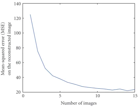
alsoSection 3.3). Therefore, the resolution can only be really increased by (almost) a factor of four. Any supplementary increase in the number of pixels can as well be performed by upsampling one of the signals and applying low-pass in-terpolation, but it does not result in an increase of resolv-ing power. It can reduce noise, however.Figure 3shows the mean-squared error (MSE) of the reconstruction versus the number of images used. The performance increases rapidly with the first six images, but the improvement is marginal beyond that.
In the rest of this paper, we will use four images as in-put to the super-resolution algorithms. Assuming the low-resolution images were subsampled by almost two, this is the theoretical limit for which our algorithm should be able to reconstruct an image of almost double resolution. In other words, four images are a minimum to have a well-determined system when upsampling by two. Thus, we do not consider the improvement to SNR that the use of more images would bring.
5. RESULTS
0 5 10 15 Number of images
20 40 60 80 100 120 140
M
ean-squar
ed
er
ro
r
(MSE)
on
the
re
const
ru
ct
ed
image
Figure3: MSE of the reconstructed image as a function of the num-ber of images used in the super-resolution algorithm. Six images form a good trade-offbetween performance and computational complexity.
In both simulation and experiment, we compared our registration algorithm to other registration methods. First, our registration method is compared to the frequency do-main algorithms by Marcel et al. [18] and by Lucchese and Cortelazzo [22]. Because Lucchese and Cortelazzo use the same phase correlation method as Marcel et al., the method by Lucchese and Cortelazzo is not included in the simula-tions where only shifts are used. Next, we also compared it to the spatial domain method based on Taylor expan-sions by Keren et al. [5]. In the simulations using only shifts, our registration method was also compared to the algorithm by Bergen et al. [24], as it was implemented in the super-resolution imaging software by Farsiu et al. [28]. This was only done for the case of horizontal and vertical shifts, be-cause image rotations are not (yet) implemented in this soft-ware.
5.1. Simulation
In the simulation, we started from a high-resolution im-age, which was considered as the equivalent for continu-ous space (Figure 5(a)). This image was then multiplied by a Tukey window (Figure 5(b)) to make the image circu-larly symmetric and thus avoiding all boundary effects. Next, three shifted and rotated copies are created from this high-resolution image. Gaussian zero-mean random variables are used for the shift (pixels) and rotation (degrees) parameters. For the shifts, a standard deviation of 2 is used, while the rotation angles have a standard deviation of 1. The different images are then low-pass filtered using an ideal low-pass fil-ter with cutofffrequency 0.12us(with usthe sampling fre-quency of the high-resolution image) to achieve the setup specified inSection 3.3andFigure 2. The first of these im-ages (not-moved reference image) will be the reconstruction target for the super-resolution algorithm (Figure 5(c)). And finally, the four images are downsampled by a factor eight.
This results in four low-resolution, shifted and rotated im-ages that can be used as input for the super-resolution algo-rithm (Figure 5(d)). They are aliasing-free in the frequency band (−0.04us, 0.04us), and are aliased in the rest of the spec-trum as discussed inSection 3.3andFigure 2. By construc-tion, all shifts are multiples of 0.125, but this information is not used in any of the registration algorithms to keep them generally applicable.
The results using the different algorithms are summa-rized inTable 1. The registration results with our algorithm are much better than the other frequency domain algorithms by Marcel et al. and Lucchese and Cortelazzo. The motion es-timates using the algorithm by Lucchese and Cortelazzo are still accurate up to subpixel precision, while the algorithm by Marcel et al. performs much worse in estimating the ro-tation angle. Because of this erroneous roro-tation cancellation, the following motion estimation also fails. The results ob-tained with the algorithm by Keren et al. are similar to those with our algorithm in both shift and rotation estimation.
Another simulation was also made with only horizontal and vertical shifts. The results of this simulation are listed inTable 2. Our algorithm outperformed the other methods and computed the parameters up to the working precision of the computations. The algorithm by Marcel et al. has clearly lower precision than the other algorithms. The spatial do-main algorithms by Keren et al. and by Bergen et al. (as im-plemented by Farsiu et al.) outperform the frequency domain algorithm by Marcel et al., but have lower precision than our algorithm.
In order to find the same motion parameters in the reg-istration as the parameters that were used to create the im-ages, we need to reverse the order in the registration. In other words, because we first shifted the images and then rotated them in the simulation setup, we need to undo the rotation first and then the shifts. Otherwise, a conversion would have to be made before comparing the two.
5.2. Practical experiment
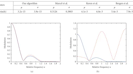
The different algorithms are also compared in two practical experiments with real images. First, a Leica DC250 black and white digital camera is used, with a Nikon 85 mm optical system. As can be seen from its spatial frequency response [29] (Figure 6), aliasing artifacts can occur with this camera. The camera was firmly fixed on a stable tripod that allows only horizontal and vertical shifts and planar rotations par-allel to the image plane.
With this camera setup, four shifted and rotated images of a planar scene are captured (Figures7(a)and7(b)1). The planar scene is a resolution test chartin a plane parallel to the image plane of the camera. These images are then registered using the different registration algorithms to be compared (see Table 3), and a high-resolution image is reconstructed using bicubic interpolation (Figure 8).
(a) (b) (c)
Figure4: High-resolution images used in the simulations. (a) Building, (b) castle, and (c) leaves.
(a) (b) (c)
(d) (e)
Figure5: Simulation setup. (a) Original high-resolution image. (b) Original image multiplied by a window to make it circularly symmetric. (c) Low-pass filtered image to satisfy the reconstruction conditions. This image is used as reconstruction target. (d) Low-resolution image used as input to the super-resolution algorithm. (e) Reconstructed high-resolution image.
In a second experiment, a set of four color images was taken using a Sigma SD10 digital camera. This camera uses a Foveon X3 sensor, which has three photodetectors (for red, green, and blue) at every pixel location. The camera was held manually in approximately the same position while taking
Table1: Comparison of the average absolute error (μ) and the standard deviation of the error (σ) for the shift and rotation parameters in the different algorithms. 150 simulations were performed for each of the images (Figure 4).
Parameters Our algorithm Marcel et al. Lucchese et al. Keren et al.
μ σ μ σ μ σ μ σ
Shift (pixels) 0.029 0.038 1.999 11.522 0.327 0.417 0.019 0.027
Rotation angle (deg) 0.126 0.191 19.003 79.086 0.142 0.181 0.053 0.071
Table2: Comparison of the average absolute error (μ) and the standard deviation of the error (σ) for the shift parameter in the different algorithms. 150 simulations with only horizontal and vertical shifts (no rotations) were performed for each of the images.
Parameters Our algorithm Marcel et al. Keren et al. Bergen et al.
μ σ μ σ μ σ μ σ
Shift (pixels) 3.2e-15 3.9e-15 0.3126 0.3803 4.1e-3 6.0e-3 5.4e-3 7.9e-3
0 0.2 0.4 0.6 0.8 1 1.2 1.4 1.6 1.8 2 Relative frequencyu
0 0.1 0.2 0.3 0.4 0.5 0.6 0.7 0.8 0.9 1
M
o
dulation
(a)
0 0.2 0.4 0.6 0.8 1 1.2 1.4 1.6 1.8 2 Relative frequencyu
0 0.2 0.4 0.6 0.8 1 1.2 1.4
M
o
dulation
(b)
Figure6: Spatial frequency response. (a) Horizontal (dashed line) and vertical (solid line) relative spatial frequency response of the Le-ica DC250 digital camera used in the experiment. A relative spatial frequency of 1 corresponds to 1017 line widths/picture height and 74 cycles/mm on the image sensor. (b) Relative spatial frequency response (solid line) and its aliased versions (dashed line) after sampling. Although there is no aliasing-free part, the signal-to-aliasing ratio is relatively high for low frequencies, and our algorithm still works.
In these experiments, the estimated cutofffrequency in our algorithm is set as high as possible to obtain reliable re-sults. The shifts are estimated from the central 5% of the fre-quency domain image, while for the rotation estimation, a disc withρ = 0.6 is used. The use of more information for the rotation estimation than for the shift estimation is re-quired to get sufficient precision (see alsoSection 6). It can be justified by the fact that in this area, the aliasing compo-nent of the sampled signal is smaller than the base spectrum component.
The estimates using the algorithm by Marcel et al. and the shift estimation of the algorithm by Lucchese and Corte-lazzo have lower precision due to the size of the images. Be-cause the original images are already relatively large, the re-quired additional upsampling and interpolation require too much memory to be performed on a regular computer. The upsampling is therefore omitted in this case and the shifts are only computed up to pixel level.
Because the exact motion parameters are unknown, it is only possible to compare visually the different reconstructed images. From Figures8and9, it can be seen that with our al-gorithm, the registration was very accurate. Most aliasing has been removed in both reconstructed images. In the images obtained with the algorithms by Marcel et al. and by Luc-chese and Cortelazzo, at least one of the images was badly aligned. Therefore, the reconstructions are also less precise. The results with the algorithm by Keren et al. are comparable to the results with our algorithm.
6. DISCUSSION
Table3: Registration parameters for the practical experiments using our algorithm, nonlinear minimization, and the algorithm by Keren et al. Experiment 1 is the experiment with the resolution chart using the Leica camera. Experiment 2 is the experiment with the outdoor scene using the Sigma camera.
Im. pairs Our algorithm Marcel et al. Lucchese et al. Keren et al.
Exp. 1 Δx Δy θ Δx Δy θ Δx Δy θ Δx Δy θ
Im2-Im1 9.24 −3.84 0.9 11.2 −4.20 1.06 9.00 −0.50 1.21 9.27 −3.86 0.92
Im3-Im1 9.74 −2.21 1.2 12.4 0.20 1.39 10.00 2.00 1.68 9.86 −2.29 1.14
Im4-Im1 10.32 −5.00 1.2 12.4 −5.00 1.39 11.25 −0.75 1.63 10.37 −5.06 1.17
Exp. 2 Δx Δy θ Δx Δy θ Δx Δy θ Δx Δy θ
Im2-Im1 −12.75 −10.34 −0.1 −17 −10 0 −15 −4 −0.53 −12.51 −10.43 −0.01
Im3-Im1 14.65 12.96 0 22 13 0 11 36 1.66 15.22 13.08 0.01
Im4-Im1 −12.08 1.54 −0.1 −18 2 0 −14 −6 −0.63 −12.76 1.74 −0.09
(a) (b)
(c) (d)
Figure7: Aliased images taken with a real digital camera and used in the practical experiments. (a) One of the four images of the res-olution chart taken with the Leica digital camera, and (b) a detail showing the aliasing. (c) One of the four images of a real-life scene taken with the Sigma digital camera, and (d) a detail showing the aliasing. The four images for both experiments are available online [30].
resolution and remove aliasing artifacts (see Figures8 and
9). Our algorithm performs better than the algorithm by Keren et al. if there is some strong directionality present in the images. The other frequency domain algorithms by Mar-cel et al. and Lucchese and Cortelazzo perform worse both in the simulations and in the practical experiment.
We can also observe that a bad image registration is fatal for the reconstruction. In such cases, it would be better to re-construct a larger image from only one of the low-resolution images using interpolation, even though this does not in-crease the resolution. The artifacts due to bad motion esti-mation are visually very noticeable.
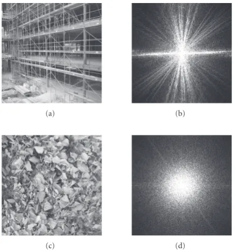
Our algorithm works best on images with strong fre-quency content in certain directions (Figures 10(a) and
10(b)). In that case, our algorithm outperforms all other al-gorithms including the spatial domain algorithm by Keren et al. The accuracy of our rotation estimation (and conse-quently also of the shift estimation) depends on the presence of some strong directionality in the images. This can be ob-served inTable 4, where the results fromTable 1for our algo-rithm are displayed per image. If such frequency directions are not present (Figures 10(c)and10(d)), the registration performance decreases. The results with our algorithm are then slightly worse than with the algorithm by Keren et al., but still much better than those using the other frequency domain algorithms. This dependence on directionality is re-lated to the projection along radial lines in our rotation es-timation algorithm. This highly reduces the computational complexity of the algorithm, as only a one-dimensional cor-relation is required instead of the regular two-dimensional correlations. However, because of the projection, it is also more subject to errors if there are no strong directions in the image.
Next to the presence of directional frequency content, the size of the low-resolution images also constrains the preci-sion of our rotation estimation algorithm. As the frequency values have to be averaged over a small angle (typically a few degrees), the number of values to be averaged will be very limited for small images. This number of values also varies for different angles (e.g., more values around 0 and 90 de-grees, less in between), which biases the computed functions. InTable 5, simulation results with our algorithm are com-pared for different image sizes. This explains also why we consider a large disc for the rotation estimation, as estimates based on the aliasing-free part alone are not accurate enough. The super-resolution technique described in Sections3
(a) (b)
(c) (d)
Figure8: Results of the different super-resolution algorithms on the real images of the resolution chart. Zoomed images of the central part are displayed to show the differences better. (a) Our algorithm. (b) Registration algorithm by Marcel et al. (c) Registration algorithm by Lucchese and Cortelazzo. (d) Registration algorithm by Keren et al.
(a) (b) (c) (d)
Figure9: Results of the different super-resolution algorithms on the images of the real-life scene. Zoomed images of the central part are displayed to show the differences better. (a) Our algorithm. (b) Registration algorithm by Marcel et al. (c) Registration algorithm by Lucchese and Cortelazzo. (d) Registration algorithm by Keren et al.
remove aliasing. An optical low-pass filter is applied to the image before it is captured to ensure that aliasing cannot oc-cur. Our technique totally relies on the presence of aliasing in
(a) (b)
(c) (d)
Figure10: Our algorithm works best on images with strong fre-quency content in a number of directions ((a) and its Fourier trans-form (b)). If the energy is homogeneously spread among all possible directions (as can be seen in (c) and its Fourier transform (d)), the performance of the motion estimation algorithm decreases.
Table4: Comparison of the average absolute error (μ) and the stan-dard deviation of the error (σ) for the shift and rotation parameters on different images. 150 simulations were performed for each of the images (Figure 4).
Parameters Image4(a) Image4(b) Image4(c)
μ σ μ σ μ σ
Shift (pixels) 0.041 0.050 0.025 0.027 0.020 0.031
Rotation angle (deg) 0.050 0.034 0.063 0.066 0.265 0.316
The advantage of a frequency domain approach is that the aliasing terms are clearly distinguishable. This makes it much easier to take aliasing into account and accurately esti-mate the motion, even in the (partially) aliased case. The fact that only low-frequency information was used makes the al-gorithm also more robust to noise, which is strongest in high frequencies.
The disadvantage of a frequency domain motion estima-tion algorithm is that it can compute only one set of moestima-tion parameters for the whole image. This motion model does not include a scenario when one object in a scene moves and the rest of the scene stays constant. For such cases, a local algo-rithm is needed.
7. CONCLUSIONS
We presented a new frequency domain method for the registration of a set of low-resolution, aliased images that
Table5: Comparison of the average absolute error (μ) and the stan-dard deviation of the error (σ) for the shift and rotation parameters for different image sizes using our algorithm. 50 simulations were performed for each of the three images (Figure 4).
Input image size 221×221 pixels 884×884 pixels
μ σ μ σ
Shift (pixels) 0.0748 0.1010 0.0288 0.0376
Rotation angle (deg) 0.3931 0.5550 0.1261 0.1910
outperforms previous frequency domain registration meth-ods. Planar rotation and translation parameters are precisely estimated based on the low-frequency, aliasing-free part of the images. This image registration technique is then ap-plied to super-resolution imaging to reconstruct a double-resolution image (in each dimension) from a set of aliased images. After the image alignment, bicubic interpolation was used to reconstruct the high-resolution image. This algorithm was compared to some other frequency and spatial domain methods in simulations and practical experiments. Both proved the validity and high precision of our algorithm. If the low-resolution images are sufficiently large and have di-rectionality, our algorithm outperforms the other algorithms and accurate aliasing-free high-resolution images can be re-constructed.
ACKNOWLEDGMENTS
The work presented in this paper was supported in part by the National Competence Center in Research on Mobile Information and Communication Systems (NCCR-MICS), a center supported by the Swiss National Science Founda-tion under Grant no. 5005-67322. All the results and fig-ures displayed in this paper are reproducible [31] using the data and Matlab code available online [30]. We thank Urs Schmid from Leica Microsystems AG and Rudy Guttosch from Foveon, Inc. for providing digital cameras, and Sina Farsiu and Peyman Milanfar from UC Santa Cruz for allow-ing us to use their super-resolution software. We would also like to thank the reviewers for their valuable comments to improve the quality of this paper.
REFERENCES
[1] R. Y. Tsai and T. S. Huang, “Multiframe image restoration and registration,” inAdvances in Computer Vision and Image Pro-cessing, vol. 1, chapter 7, pp. 317–339, JAI Press, Greenwich, Conn, USA, 1984.
[2] P. Vandewalle, S. E. S¨usstrunk, and M. Vetterli, “Super-resolution images reconstructed from aliased images,” in ceedings of SPIE/IS&T Visual Communications and Image Pro-cessing Conference, T. Ebrahimi and T. Sikora, Eds., vol. 5150 ofProceedings of SPIE, pp. 1398–1405, Lugano, Switzerland, 2003.
[4] D. Capel and A. Zisserman, “Computer vision applied to super-resolution,”IEEE Signal Processing Magazine, vol. 20, no. 3, pp. 75–86, 2003.
[5] D. Keren, S. Peleg, and R. Brada, “Image sequence enhance-ment using sub-pixel displaceenhance-ments,” inProceedings of IEEE Computer Society Conference on Computer Vision and Pattern Recognition (CVPR ’88), pp. 742–746, Ann Arbor, Mich, USA, June 1988.
[6] R. R. Schultz, L. Meng, and R. L. Stevenson, “Subpixel mo-tion estimamo-tion for super-resolumo-tion image sequence enhance-ment,”Journal of Visual Communication and Image Represen-tation, vol. 9, no. 1, pp. 38–50, 1998.
[7] M. Irani and S. Peleg, “Improving resolution by image reg-istration,” CVGIP: Graphical Models and Image Processing, vol. 53, no. 3, pp. 231–239, 1991.
[8] D. Rajan, S. Chaudhuri, and M. V. Joshi, “Multi-objective super-resolution: concepts and examples,”IEEE Signal Process-ing Magazine, vol. 20, no. 3, pp. 49–61, 2003.
[9] M. V. Joshi, S. Chaudhuri, and R. Panuganti, “Super-resolution imaging: use of zoom as a cue,”Image and Vision Computing, vol. 22, no. 14, pp. 1185–1196, 2004.
[10] A. J. Patti, M. I. Sezan, and A. Murat Tekalp, “Super-resolution video reconstruction with arbitrary sampling lattices and nonzero aperture time,”IEEE Transactions on Image Process-ing, vol. 6, no. 8, pp. 1064–1076, 1997.
[11] A. Zomet, A. Rav-Acha, and S. Peleg, “Robust super-resolution,” inProceedings of IEEE Computer Society Confer-ence on Computer Vision and Pattern Recognition (CVPR ’01), vol. 1, pp. 645–650, Kauai, Hawaii, USA, December 2001. [12] S. Farsiu, M. D. Robinson, M. Elad, and P. Milanfar, “Fast and
robust multiframe super-resolution,”IEEE Transactions on Im-age Processing, vol. 13, no. 10, pp. 1327–1344, 2004.
[13] M. Elad and A. Feuer, “Restoration of a single super-resolution image from several blurred, noisy, and undersampled mea-sured images,”IEEE Transactions on Image Processing, vol. 6, no. 12, pp. 1646–1658, 1997.
[14] S. Borman and R. L. Stevenson, “Spatial resolution enhance-ment of low-resolution image sequences—a comprehensive review with directions for future research,” Tech. Rep., Lab-oratory for Image and Signal Analysis (LISA), University of Notre Dame, Notre Dame, Ind, USA, 1998. Online available: http://www.nd.edu/∼sborman/publications/.
[15] S. C. Park, M. K. Park, and M. G. Kang, “Super-resolution im-age reconstruction: a technical overview,”IEEE Signal Process-ing Magazine, vol. 20, no. 3, pp. 21–36, 2003.
[16] B. Zitov´a and J. Flusser, “Image registration methods: a sur-vey,”Image and Vision Computing, vol. 21, no. 11, pp. 977– 1000, 2003.
[17] B. S. Reddy and B. N. Chatterji, “An FFT-based technique for translation, rotation, and scale-invariant image registration,” IEEE Transactions on Image Processing, vol. 5, no. 8, pp. 1266– 1271, 1996.
[18] B. Marcel, M. Briot, and R. Murrieta, “Calcul de translation et rotation par la transformation de Fourier,”Traitement du Signal, vol. 14, no. 2, pp. 135–149, 1997.
[19] S. P. Kim and W.-Y. Su, “Subpixel accuracy image registration by spectrum cancellation,” inProceedings of IEEE International Conference Acoustics, Speech, Signal Processing (ICASSP ’93), vol. 5, pp. 153–156, Minneapolis, Minn, USA, April 1993. [20] H. S. Stone, M. T. Orchard, E.-C. Chang, and S. A. Martucci,
“A fast direct Fourier-based algorithm for subpixel registration of images,”IEEE Transactions on Geoscience and Remote Sens-ing, vol. 39, no. 10, pp. 2235–2243, 2001.
[21] H. Foroosh, J. B. Zerubia, and M. Berthod, “Extension of phase correlation to subpixel registration,”IEEE Transactions on Image Processing, vol. 11, no. 3, pp. 188–200, 2002. [22] L. Lucchese and G. M. Cortelazzo, “A noise-robust frequency
domain technique for estimating planar roto-translations,” IEEE Transactions on Signal Processing, vol. 48, no. 6, pp. 1769– 1786, 2000.
[23] M. A. Fischler and R. C. Bolles, “Random sample consensus: a paradigm for model fitting with applications to image analy-sis and automated cartography,”Communications of the ACM, vol. 24, no. 6, pp. 381–395, 1981.
[24] J. R. Bergen, P. Anandan, K. J. Hanna, and R. Hingorani, “Hierarchical model-based motion estimation,” in Proceed-ings of 2nd European Conference on Computer Vision (ECCV ’92), Lecture Notes in Computer Science, pp. 237–252, Santa Margherita Ligure, Italy, May 1992.
[25] M. Irani, B. Rousso, and S. Peleg, “Computing occluding and transparent motions,”International Journal of Computer Vi-sion, vol. 12, no. 1, pp. 5–16, 1994.
[26] J. Gluckman, “Gradient field distributions for the registration of images,” inProceedings of IEEE International Conference on Image Processing (ICIP ’03), vol. 3, pp. 691–694, Barcelona, Spain, September 2003.
[27] A. Papoulis, “Generalized sampling expansion,”IEEE Transac-tions on Circuits Systems, vol. 24, no. 11, pp. 652–654, 1977. [28] S. Farsiu, M. D. Robinson, and P. Milanfar, “MDSP
res-olution enhancement software,” 2004, Online available: http://www.soe.ucsc.edu/∼milanfar/SR-Software.htm. [29] International Organization for Standardization, “ISO
12233:2000—Photography—Electronic still picture cameras —Resolution measurements,” 2000.
[30] http://lcavwww.epfl.ch/reproducible research/ VandewalleSV05/.
[31] M. Schwab, M. Karrenbach, and J. Claerbout, “Making scien-tific computations reproducible,”Computing in Science & En-gineering, vol. 2, no. 6, pp. 61–67, 2000.
Patrick Vandewalle received the M.S. degree in electrical engineering from Katholieke Universiteit Leuven, Belgium in 2001. From 2001 to 2002, he worked as a Research Assistant in the Medical Imaging Lab at the Department of Electrical Engi-neering (ESAT), KU Leuven. He is currently pursuing the Ph.D. degree in computer, communication, and information sciences at the Ecole Polytechnique F´ed´erale de
Lausanne (EPFL), Lausanne, Switzerland. His research interests are in signal and image processing, sampling, and digital photography.
Sabine S¨usstrunkreceived the B.S. degree in scientific photography from the Swiss Federal Institute of Technology, Zurich, Switzerland, and the M.S. degree in graphic arts publishing, concentration in electronic publishing, from the Rochester Institute of Technology, Rochester, NY, and the Ph.D. in computer science from the University of East Anglia, Norwich, UK in 1987, 1993, and 2005, respectively. She is an Adjunct
Switzerland. Her research interests are in digital photography, color image processing, and image quality.
Martin Vetterli received his Engineering degree from ETH Zurich, Switzerland, his M.S. degree from Stanford, and his Ph.D. degree from Ecole Polytechnique F´ed´erale de Lausanne. In 1986, he joined Columbia University in New York, first with the Cen-ter for Telecommunications Research and then with the Department of Electrical En-gineering where he was an Associate Pro-fessor of electrical engineering. In 1993, he