Volume 2006, Article ID 86053, Pages1–13 DOI 10.1155/ASP/2006/86053
Target Identification Using Harmonic
Wavelet Based ISAR Imaging
B. K. Shreyamsha Kumar, B. Prabhakar, K. Suryanarayana, V. Thilagavathi, and R. Rajagopal
Central Research Laboratory, Bharat Electronics Limited, Bangalore-560013, India
Received 30 April 2005; Revised 21 November 2005; Accepted 23 November 2005
A new approach has been proposed to reduce the computations involved in the ISAR imaging, which uses harmonic wavelet-(HW) based time-frequency representation (TFR). Since the HW-based TFR falls into a category of nonparametric time-frequency (T-F) analysis tool, it is computationally efficient compared to parametric T-F analysis tools such as adaptive joint time-frequency transform (AJTFT), adaptive wavelet transform (AWT), and evolutionary AWT (EAWT). Further, the performance of the proposed method of ISAR imaging is compared with the ISAR imaging by other nonparametric T-F analysis tools such as short-time Fourier transform (STFT) and Choi-Williams distribution (CWD). In the ISAR imaging, the use of HW-based TFR provides similar/better results with significant (92%) computational advantage compared to that obtained by CWD. The ISAR images thus obtained are identified using a neural network-based classification scheme with feature set invariant to translation, rotation, and scaling.
Copyright © 2006 Hindawi Publishing Corporation. All rights reserved.
1. INTRODUCTION
Inverse synthetic aperture radar (ISAR)is an imagingradar that uses the target’s pitch, roll, and yaw motions to gen-erate an image in the range-Doppler plane. Primarily, the Fourier transform (FT) was used for the ISAR imaging with the assumption that Doppler frequency is constant over the imaging time duration [1,2]. However, the assumption of constant Doppler frequency is not true as the Doppler fre-quency varies in time because of the nonuniform motion of the target due to maneuvers. Hence the FT-based method suffers from the disadvantage of image blurring in the final output.
In the last decade, many techniques such as transform domain methods, subaperture methods, and superresolution methods have been applied to obtain the time-varying spec-trum in the hope of enhancing image resolution. How-ever, none of them completely resolved the blurring prob-lem. With the intention of obtaining focused ISAR image, Chen et al. introduced time-frequency (T-F) transform in the place of FT. Well-known T-F transforms include short-time Fourier transform (STFT), Wigner-Ville distribution (WVD) [1, 2], continuous wavelet transform (CWT) [3], adaptive joint time-frequency transform (AJTFT) [4], adap-tive wavelet transform (AWT) [5], and evolutionary AWT (EAWT) [6]. Among these T-F transforms, STFT, WVD, and CWT fall into a category of nonparametric T-F anal-ysis tools whereas AJTFT, AWT, and EAWT fall into a
category of parametric T-F analysis tools. The STFT is the best-known and most basic T-F analysis tool, but it suffers from tradeoffbetween time resolution and frequency resolu-tion. The WVD [7,8] provides better resolution both in time as well as frequency, but has a cross-term problem. The CWT has multiresolution characteristics and it is free from cross-term problem, but its T-F grid is still rigid [2,6]. The AWT provides a more flexible T-F grid than the CWT. Further, it is free from resolution problem and cross-term problem, but its accuracy is limited as it uses a bisection search method and fast FT (FFT) for parameter extraction [5]. The AJTFT uses iterative search method to get the adaptive spectrogram (ADS) [2,4] that is in turn used to extract feature set for target recognition without computing the ISAR image. The EAWT uses evolutionary programming for the T-F parame-ter extraction instead of FFT and the bisection search method used in the conventional AWT [5]. As all the parametric T-F analysis tools [2,4–6] use parameter extraction as well as one or the other search methods while getting ISAR image, the computational complexity involved is quite high and hence hard to realize in real-time applications [6].
and is difficult to implement for practical scenarios. In [9], Newland modified the harmonic wavelets (HW) [10–12] for time-frequency representation (TFR), which issimple to im-plementcompared to other wavelets and TFRs like WVD and CWD.
In order to trim down thecomputational complexity as-sociated with ISAR imaging and make itviablefor practical applications, the conception of TFR by HW is proposed in this paper for ISAR imaging. To capture theDoppler informa-tioneffectively,high-frequency resolutionis required, which is achieved withshorter frequency window functionwhile com-puting the TFR by HW. The results from the simulated ISAR data show that the proposed method providesbetter image compared to that generated by CWD with reduction in com-putational complexity. Since the cost of the comcom-putational complexity plays an important role for practical scenarios, the proposed method is well suited for real-time implemen-tation. The ISAR image thus obtained from the proposed method can be used for target identification using any of the existing methods. Here the neural network-based automatic target identification (ATI) scheme invariant to translation, rotation, and scale is used for identification and classifica-tion.
ATI is an important problem in the field of machine learning and pattern recognition. Hence, in the last two decades a large number of algorithms have been proposed. For example, Oja used the principle component analysis technique [13], Comon adopted the independent compo-nent approach [14], and Al-Ani et al. proposed a hybrid in-formation algorithm [15] to deal with the problem of fea-ture selection. Several methods were also proposed based on probability theory [16], fuzzy set theory [17], and artificial neural networks (ANNs) [18–20]. Further, the target recog-nition scheme discussed in [4] extracts the feature set directly from geometrical moments of the ADS without computing the ISAR image. But, the proposed method of recognition uses ISAR image for extracting the feature set. As the ISAR image gives the silhouette of the target, the trained operator can use his intelligence in addition to machine intelligence in classification and decision-making.
Any recognition process usually involves three compo-nents: preprocessing block, feature extractor, and classifier. The function of preprocessing block is to transform the input digital image into a form that can be processed and used by the subsequent blocks. Typical image-preprocessing func-tions are noise suppression, blur control, edge detection, and boundary extraction. In feature extractor, certain selective characteristics of the image are extracted that can uniquely distinguish the image from the other class of images. If the selected feature set is large, the preprocessing and analysis task becomes more difficult. On the other hand, if the feature set is small, the recognition rate may come down. Also, the extracted features should be invariant to certain parameters like scaling, shifting, and rotation depending on the scenario. As a result, feature selection has become important and well-known problem. The classifier block compares these features with the feature set in the database according to a
prede-fined similarity function and classifies the output image to one class of the stored images.
In this paper, region-growing technique is used for finding the centroid to overcome the problem of spurious edges and noise. A rotation invariant, translation invariant, and scale invariant feature set is selected for accurate clas-sification [21]. Neural network-based clasclas-sification is done instead of conventional template matching to increase the speed of matching and robustness to distorted patterns.
This paper is organized as follows. The basic of HW and its variation for ISAR imaging is discussed inSection 2. Neural network-based ATI using ISAR images invariant to translation, rotation, and scaling is discussed in Section 3. Section 4 presents simulated results for ISAR imaging and classification. Finally conclusions are made inSection 5.
2. ISAR IMAGING USING TIME-FREQUENCY REPRESENTATION
Radar transmits electromagnetic waves to a target and re-ceives the reflected signal from the target. The received signal can be used to obtain the image of the target as it is related to the reflectivity function of the target by means of a filter-ing process.Figure 1illustrates the process of the ISAR imag-ing system usimag-ing a stepped-frequency (SF) waveform. For a stepped-frequency waveform, the radar transmits a sequence ofN bursts. Each burst consists ofM narrow-band pulses. Within each burst, the center frequency fmof each successive pulse is increased by a constant frequency stepΔf. The total bandwidth of the burst, that is,M times the frequency step Δf, determines the radar range resolution. The total number of burstsNalong with the pulse duration for a given imaging integration time determine the Doppler or cross-range res-olution. The returned pulse is heterodyned and quadrature detected in the radar receiver.
To form a radar image, after measuring the returned in-phase (I-Channel) and quadrature phase (Q-Channel) sig-nals at baseband with a pulse repetition rate atM∗Ntime instants tm,n = (m+nM)Δt, the M×N complex data is organized into a two-dimensional array which represents the unprocessed spatial frequency signature of the targetS(fm,n), wherem= 1, 2,. . .,M,n= 1, 2,. . .,N, andΔtdenotes the time interval between the pulses.
The radar processor uses the frequency signatures as the raw data to perform range compression and the stan-dard motion compensation. Range compression functions as a matched filter, which removes frequency or phase mod-ulation and resolves range. For the stepped-frequency sig-nals, the range compression performs an M-point inverse FT (IFT) for each of theN received frequency signatures as
G(rm,n)=IFTm{S(fm,n)}, where IFTmdenotes the IFT oper-ation with respect to the variablem. Therefore,Nrange pro-files (i.e., the distribution of the target reflectivity in range), each containingMrange cells, can be obtained. At each range cell, theN range profiles constitute a new time history se-ries. Then, the motion compensated range profiles become
Mpulses
Transmitted stepped-frequency signal
T no1 no2 f Nbursts
R R
ρ(x,y)
Moving target
Time history
1 2 . . . N
M . . . 2 1
F
req
uency
sig
natur
e
2R/c
T f
Received signal Range gates
N M
Motion compensation
N M
Range compression IFT
M Doppler
processing JTF M
range
N Doppler Radar image
Figure1: Illustration of SF radar imaging of moving target.
2.1. Time-frequency representation
TFR is an essential element in most of diagnostic sig-nal asig-nalysis schemes. There is considerable interest in the effectiveness of different methods for generating TFRs, which describe the distribution of energy over frequency and time. The three main methods are: (1) the short-time Fourier transform (STFT), which generates a spectrogram, (2) the Wigner-Ville method of generating time-frequency distribu-tions, and (3) the harmonic wavelet (HW) method of con-structing wavelet maps, which is akin to TFR except that wavelet scale is plotted instead of frequency. All three meth-ods generate a (real) function of time and frequency, which can be plotted to generate a surface on the time-frequency plane. For this purpose, wavelet scale is converted to fre-quency.
The Wigner-Ville distribution (WVD) is a TFR with ex-cellent time and frequency resolution and several translation, modulation and marginal properties, and hence, is very use-ful for nonstationary signal analysis. The WVD of a signal
x(t) is given by [7,8]
Wx(t,ω)=
∞
−∞r(t,τ)e
−jωτdτ, (1)
wherer(t,τ) = x(t+τ/2)x∗(t−τ/2) is called the instan-taneous autocorrelation function and the superscript∗ in-dicates conjugate operation. Since the lag length τ can go to even infinity, the WVD theoretically can provide infinite frequency resolution. The WVD has two fundamental dis-advantages: (1) computational complexity and (2) difficulty introduced by its spurious interference terms (cross-terms). The former is an important practical problem and the lat-ter occurs when the signal contains more than one compo-nent because of the built-in quadratic nature of the WVD.
For real-time computations or for long-time series, this leads to inaccuracies and hence, it can be reduced by filtering the WVD with Choi-Williams kernele−θ2τ2/σ
. This filtered WVD is also known as Choi-Williams distribution (CWD) as it uses Choi-Williams kernel to reduce the cross-terms and preserve the useful properties of the WVD with slightly re-duced time-frequency resolution and largely rere-duced cross-term interference. The CWD of a signalx(t) is given by [7,8]
CWD(t,ω)
= 1
4π3/2
1
√
τ2/σ exp
−(u−t)2
4τ2/σ −jτω
r(u,τ)du dτ.
(2)
For large values ofσ, CWD approaches the WVD since the kernel approaches one and for small values ofσ, the cross-term existing in WVD is reduced in CWD. But, this intro-duces extra computations.
2.2. Harmonic wavelets [9,10]
In essence, HW-based TFR is the same as the STFT except that any basis function can be used (only harmonic functions of constant amplitude and phase are used by the STFT). Usu-ally the wavelets with a narrow frequency band are effective for time-frequency analysis; otherwise good frequency res-olution is impossible. Subject to this narrow-band proviso, wavelets of any kind may be used for TFR, but HWs are par-ticularly suitable because their spectrum is confined to a com-pact frequencyband.
a(n),n=0 toN−1 IFFT A(k)=
W∗(l−k+ 1)∗X(l),k≤l≤(L+k−1) 0, otherwise
W∗(l−k+ 1)=0,k≤l≤(L+k−1) L=window length
X(l),l=0 toN−1 x(n),n=0 toN−1
FFT
Figure2: Schematic to compute harmonic wavelet coefficients.
admissibility and regularity conditions [22]. For an analyz-ing wavelet functionw(t), the wavelet transform coefficient
a(t) of a signalx(t) is given by
a(t)=
∞
−∞x(τ)w(t+τ)dτ. (3)
In terms of FT,
A(ω)=X(ω)W∗(ω), (4)
a(t)=F−1X(ω)W∗(ω). (5)
That is, the wavelet transform coefficients can be computed using inverse fast Fourier transform (IFFT) algorithm by (5) usingX(ω) withW(ω) for different wavelet functions. Specifically, for the HW given by Newland [10,11],W(ω) is very simple and it is zero except over a finite band [π/ p,π/q], wherep,qcan be real numbers, not necessarily integers. For HW, the rectangular windowW(ω), though compact in fre-quency domain, is of infinite duration in time domain. This can be overcome by using a proper smoother weighing func-tionW(ω) other than a rectangular one.
A practical computation of HW for an input signalx(t) sampledN times is illustrated inFigure 2. In first stage, the FFT of the signal is computed. In second stage, the Fourier coefficients obtained are weighed by a frequency window function of lengthLand the length of the resultant block is made equal toNby paddingpleading zeros andN−(L+p) trailing zeros. The IFFT of the resultingNterm series is then computed in third stage to determine the HW coefficients (HWCs) for that particular frequency band. Similar proce-dure is repeated for the successive frequency blocks by mov-ing the frequency window along the frequency spectrum. It is shown in [9] that the number of added zeros both be-fore and after the embedded block of Fourier coefficients can be changed while still preserving the HWCs. The data in the chosen frequency band is zero-padded to get smoothness over time, which can be further improved by multiplying the
FTs of a wider range of test functions, but data for equally-spaced times is always produced. Therefore, there is a duality between the STFT and HW method. The STFT produces re-sults for local, short-time segments, covering the whole fre-quency spectrum in constant bandwidth steps whereas the HW method produces results for local, narrow frequency bandwidths, covering the whole duration of the record in constant time steps.
Both the STFT and WVD/CWD methods are constant bandwidth methods. Their algorithms require a transforma-tion from the time domain to frequency domain by using the FT generating Fourier coefficients for frequencies at constant separation. The bandwidth of each frequency term is same. In contrast, the HW method allows the bandwidth of adja-cent frequency terms to be chosen arbitrarily. Because the wavelet transform acts as a variable Q filter, where Q is the ra-tio of center frequency to bandwidth, it has greater flexibility than the other two methods. Further, the HW provides built-in decimation as well as built-interpolation if required [11,12].
The fundamental advantage of the HW is that it offers a computationally efficient method for a variable bandwidth frequency transform so that the TFR can have a constant-Q or a variable-constant-Q basis as desired. In contrast, a TFR con-structed by the STFT always has a constant bandwidth ba-sis, therefore giving the same frequency resolution from low frequencies to high frequencies. Similar to STFT, the pro-posed method also suffers from tradeoffbetween time and frequency resolution. However, to capture the Doppler in-formation effectively, better frequency resolution is required, which is achieved with shorter frequency window function while computing the HWCs.
2.3. Harmonic wavelets for ISAR imaging
In the proposed method, the HW-based TFR is customized for the purpose of ISAR imaging. Here all the stages of the HW method are similar but some extra step has to be fol-lowed before the second stage. That is, if length of the win-dow used to truncate the spectrum of the signal isL (assum-ingLas even), thenL/2 zeros have to be padded before and after the spectrum of the signal so that total length of the modified spectrum is equal to the sum of lengths of the orig-inal spectrum and the window. IfLis odd, then (L−1)/2 zeros have to be padded before and (L+ 1)/2 zeros have to be padded after the spectrum. To capture the Doppler in-formation, better frequency resolution is required, which is achieved by using a shorter window. As the window length is constant for different center frequencies, the TFR obtained by HW is of constant bandwidth just like that obtained by STFT and WVD/CWD.
The data consists ofNrange profiles each containingM
range cells. The samples taken at theith range cell for theN
range profiles constitute a time history series. For the compu-tation of a TFRi(n,k), (n =1, 2,. . .,N,k =1, 2,. . .,N), for ith range cell, HW uses this time history series as an input to get
TFRi(n,k)=IFFT
where
Ak(l)=
⎧ ⎪ ⎪ ⎨ ⎪ ⎪ ⎩
W(l−k+ 1)∗X(l),
k≤l≤(L+k−1), L: window length,
0, otherwise.
(7)
This procedure is repeated for each range cell i to get M
number of TFRs. Finally, the ISAR image atmth instant is obtained by
I(m,k)=
⎡ ⎢ ⎢ ⎢ ⎢ ⎢ ⎣
TFR1(m,k)
TFR2(m,k)
.. . TFRM(m,k)
⎤ ⎥ ⎥ ⎥ ⎥ ⎥
⎦, k=1, 2,. . .,N. (8)
Since TFRi(m,k) captures the Doppler for every time instant, the imageI(m,k) obtained by TFRi(m,k) through (8) will be of better quality with reduced blurring.
2.3.1. Algorithm for ISAR imaging by harmonic wavelets
Step 1. The given data consists ofNrange profiles each con-tainingM range cells. Compute the FT ofith range cell by
X(l) = FFT[xi(n)], wherexi(n) = x(i,n),n = 1, 2,. . .,N; i=1, 2,. . .,M, andlis the discrete frequency bin index.
Step 2. Pad the equal number of zeros at thebeginning and at theendof thespectrumof the signal such that the length of the modified spectrum is equal to the sum of lengths of the original spectrum (N) and the window (L), that is, (N+L), therefore discrete frequency bin indexl =1, 2,. . ., (N+L). This is to preserve the spectral information that may be lost otherwise.
Step 3. Compute the TFR of ith range cell using HW. For this:
(i) compute the weighted Fourier coefficients at thekth discrete frequency index using
Ak(l)=
⎧ ⎨ ⎩
W(l−k+ 1)∗X(l), k≤l≤(L+k−1),
0, otherwise, (9)
whereW(p) is the window of lengthL,p=1, 2,. . .,L, (ii) the HWCsak(n) are computed by taking IFFT of
Ak(l),
(iii) squared magnitudes of the HWCs are computed by TFRi(n,k)= |ak(n)|2,
(iv) repeat steps (i), (ii), (iii) for different frequency in-dicesk=1, 2,. . .,Nto get the complete TFR of theith range cell.
Step 4. Repeat steps 1,2, 3 to get TFRi(n,k) for different range cellsi=1, 2,. . .,M.
Table1: Computational complexity by different methods.
Number of Number of
multiplications additions STFT 3276800=32.768∗105 3145728=31.45728∗105
CWD 44058624=440.58624∗105 44040192=440.40192∗105
HW 3456636=34.56636∗105 3440252=34.40252∗105
Step 5. The range-Doppler image frame atnth time instant is obtained by combining the respectiventh Doppler spectrum from each of TFRi(n,k) fori=1, 2,. . .,M.
Steps1to5form the algorithm for ISAR imaging by HW.
2.3.2. Computational complexity
To compare the computational complexity of ISAR imaging by STFT, CWD, and HW, the data ofN range profiles each withMrange cells is considered. The computation of a sin-gle TFR by STFT requires “N”N-point FFTs for each time history. Hence the computation of “M” TFRs for each time history requires “(N∗M)”N-point FFTs. Further, the use of any window of lengthLsrequires (N∗Ls)multiplicationsfor the computation of a single TFR and thus the computation of “M” TFRs requires [(N∗Ls)∗M]multiplications. From these “M” TFRs, “M” ISAR images can be obtained.
The computation of a single TFR by CWD involves (N2
w/8)multiplications(to compute instantaneous autocor-relation function), “Nw”Nw-point IFFTs(to compute ambi-guity function), (Nw ∗Nw)multiplications (for cross-term reduction by windowing), and “(2∗Nw)”Nw-point FFTs (2-DFFT of sizeNw×Nw), whereNw=2∗N. Accordingly, the computation of “M” TFRs needsMtimes the above compu-tations, that is, [(N2
w/8) +(Nw∗Nw)]∗Mmultiplicationsand [Nw+ (2∗Nw)]∗Mnumber ofNw-point FFTs.
On the other hand, the computation of a single TFR by HW requires oneN-pointFFT and “N” (N+L)-point IFFTs for each time history. Also, the use of window of lengthLfor the computation of a single TFR requires (N∗L) multipli-cations. Consequently, the computation of “M” ISAR images requires [(N∗L)∗M]multiplications, “M”N-point FFTs, and “(N∗M)” (N+L)-point FFTs.
As the FFT lengths are different for different methods, the computational complexities involved in the methods are compared in terms of multiplications and additions. For this, the computation of a singleN-pointFFT requires 2∗N∗
log2(N) real multiplications and 2∗N∗log2(N) real addi-tions.Table 1shows the computations required by different methods in terms of multiplications and additions for the following parameters:N=64,M=64,L=4,Ls=32, and
Nw=2∗N=128.
Digital image F(x,y)
Image preprocessing
g(x,y)
Feature selection and extraction
F
Classification
C
Figure3: Typical image pattern recognition system.
the proposed method is better suited for practical scenar-ios with reduction in computations while maintaining simi-lar/better results compared to CWD.
3. TARGET RECOGNITION
A typical pattern recognition process usually involves three components, preprocessing block, feature extractor, and a classifier.Figure 3shows the block diagram of a typical im-age pattern recognition system. Input to the system is a dig-ital image. However, this image may not be in a state that can be processed. The function of image preprocessing block is to transform this input digital image f(x,y) into a form
g(x,y) that can be processed and used by the subsequent blocks. Typical image-preprocessing functions required are noise suppression, blurring control, and edge detection.
In most cases, entire image may not be required for car-rying out the pattern recognition process. Certain selective characteristics of the image can retain the uniqueness of the image. Such characteristics are called primitive features. These primitive features are to be extracted from the pre-processed image. Further, a typical recognition system needs to recognize only few classes of objects. Hence, among the primitive features, only certain features of the image (F) can uniquely distinguish it from the other classes of image. These features are identified and selected by the feature extraction block of the system shown inFigure 3. The classifier block then compares these features with the features of the image in its database according to a predefined “similarity” func-tion and recognizes the output image.
ATI using ISAR images is a challenging task because of low SNR, poor resolution, and blur associated with the ISAR images. So preprocessing block is essential before fea-ture extraction and classification. Median filtering [23] is used for removing the point-spread noise. Unwanted patches are removed and the object is extracted using the standard region-growing technique [24]. After the object is extracted from background with region-growing method, all the pixel positions within the region of interest (ROI) are well known. Giving equal importance to all the pixels within ROI, cen-troid calculation reduces to simple average of all horizontal and vertical positions of the pixels within ROI. Features are extracted from the test patterns by applying FFT and wavelet transforms to the polar-transformed original patterns. Fi-nally classification is done using the neural networks.
3.1. Feature selection and extraction
For feature selection, both Fourier descriptors and wavelet descriptors are considered. Fourier descriptor has been a
powerful tool for recognition because it has a useful prop-erty of shift invariance with respect to spectrum. However, the frequency information obtained from the Fourier de-scriptor is global, a local variation of the shape can affect all Fourier coefficients. In addition, Fourier descriptor does not have a multiresolution representation. On the other hand, wavelet descriptors have multiresolution property, but they are not translation invariant. A small shift of original signal will cause totally different wavelet coefficients. Since Fourier descriptor and wavelet descriptor both have good properties and drawbacks, they are combined to obtain the descriptor, which is invariant to translation, rotation, and scaling.
Feature extraction is a crucial processing step for pattern recognition. Some methods extract 1-D features from 2-D patterns. The advantage of this approach is that space can be saved for the database and the time for matching through the whole database can be reduced. The apparent drawback is that the recognition rate may not be very high because less information from the original pattern is retained. In this paper, 2-D features for pattern recognition is used in order to achieve higher recognition rate [25].
The translation invariance is achieved by translating the origin of the coordinate system to the center of the image pattern or object, denoted by (x0,y0). As the center of the
object is considered as the reference point for the next level processing, the recognition scheme is invariant to translation of the object within the frame.
The scale invariance is obtained by transforming the im-age pattern f(x,y) into normalized polar coordinate system. Let
d= max
f(x,y)=0
x−x0
2
+y−y0 2
(10)
be the longest distance from (x0,y0) to a point (x,y) on the
pattern.N concentric circles are drawn centered at (x0,y0)
with radius d∗I/N,I = 1, 2, 3. . .,N. Also, N angularly equal-spaced radial vectors θj departing from (x0,y0) with
angular step 2π/Nare drawn. For any small region,
Si,j=
(r,θ)|ri< r≤ri+1, θj< θ≤θj+1
,
i=0, 1,. . ., (N−1), j=0, 1,. . ., (N−1) (11)
calculate the average value of f(x,y) over this region, and as-sign the average value tog(r,θ) in the polar coordinate sys-tem. The featureg(r,θ) obtained in this way is invariant to scaling, but the rows may be circularly shifted if we use dif-ferent orientation.
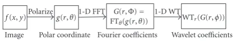
f(x,y) Image
Polarize g(r,θ)
Polar coordinate
1-D FFT G(r,Φ)= FTθ(g(r,θ))
Fourier coefficients 1-D WT
WTr(G(r,φ))
Wavelet coefficients Figure4: Block diagram of feature extraction algorithm.
level feature set. Lifting scheme is used for implementing the Haar wavelet transform because of its less computational complexity and memory requirements.
3.1.1. Feature extraction algorithm
The steps of the algorithm can be summarized as follows (also shown inFigure 4):
(1) find the centroid of the pattern f(x,y) and transform
f(x,y) into polar coordinate system to obtaing(r,θ), (2) conduct 1-D FT ong(r,θ) along the axis of polar angle
θand obtain its spectrum,
(3) apply 1-D wavelet transform onG(r,Φ) along the axis of radiusr.
3.2. Neural network-based pattern recognition
Back propagation network is an ideal choice to serve as a pattern classifier because it has been used successfully in var-ious pattern recognition applications with good recognition results. In the back propagation algorithm, the information about errors at the output units is propagated back to the hidden units. The number of input units depends on the size of feature vector. The training of a network by back propaga-tion involves three stages: the feed forward of the input train-ing pattern, the calculation and back propagation of the as-sociated error, and the adjustment of the weights. Through a set of learning samples, the network can find the best weights
Wi j automatically, enabling it to exhibit optimal classifica-tion ability. After training, applicaclassifica-tion of the net involves only computations of the feed forward phase. Even if training is slow, a trained net can produce its output very rapidly.
Feature vectors coming from feature selection and extrac-tion block are given as input to the neural network. Back propagation network with one input layer, one hidden layer, and one output layer is used for classification. The activa-tion funcactiva-tion used is a binary sigmoidal funcactiva-tion, which has a range of (0, 1) and is defined as
f(x)= 1
1 +e−x,
f(x)= f(x)1−f(x).
(12)
The initial weights are set at random. In the training process, weights are updated in such a way as to mini-mize the mean square difference between the actual and de-sired output. Finally the pattern is classified according to the output sequence of the neural network.
4. SIMULATION RESULTS
The radar data used for simulation is obtained from the stepped-frequency radar operating at 9 GHz and has a band-width of 512 MHz (for MIG-25), 150 MHz (for B-727) [http://airborne.nrl.navy.mil/∼vchen/tftsa.html]. The radar data of MIG-25 consists of 512 successive pulses with each pulse having 64 complex range samples and that of B-727 consists of 256 successive pulses with each pulse having 64 complex range samples.
The performance of the proposed method of ISAR imag-ing is compared with the existimag-ing methods usimag-ing FT, STFT, and CWD and is illustrated for both the aircrafts. Figures5 and6illustrate the performance comparison of the proposed method for MIG-25. Use of FT for ISAR imaging assumes that Doppler frequency is constant over the imaging time duration. However, the assumption of constant Doppler fre-quency is not true as the Doppler frefre-quency varies in time because of the nonuniform motion of the target. Hence the ISAR image computed by FT often leads to blurring, which is illustrated inFigure 5(a). The ISAR images (frame 30) ob-tained by STFT, CWD, and HW are shown in Figures5(b), (c), and (d), respectively. It is observed that the ISAR im-age obtained by CWD (Figure 5(c)) is prolonged in Doppler frequency. This is because the spectral peaks will occur at twice the desired frequencies due to built-in nature of the WVD. Even though the proposed method requires one ex-tra FT (to compute the spectrum of the signal for a sin-gle TFR) compared to STFT, it provides better Doppler fre-quency resolution. Further, ISAR image by HW provides bet-ter Doppler frequency resolution compared to CWD, with reduced computations.
The blurred ISAR image obtained by FT of frame-1 is shown in Figure 6(a). The frame-1 images of MIG-25 obtained by CWD and STFT are of poor quality com-pared to that obtained by HW (Figure 6). That is, the pro-posed method gives better image quality compared to other nonparametric methods with reduced computations. Sim-ilar results are shown in Figure 7(frame-30) and Figure 8 (frame-1) for B-727 to compare the performance of the pro-posed method with the existing methods. Because of the complex motion of the target B-727, the image by FT suf-fers from blurring (Figures7(a),8(a)), which is not observed in other methods (Figures7(b), (c), (d)). Also, it is observed that images obtained by STFT and CWD do not show the wings, wingtips, and tail of the target clearly (Figures7(b), (c),8(b), (c)), but are visible to some extent with HW (Fig-ures7(d),8(d)). Further, the proposed method provides bet-ter and consistent results for all the frames compared to other two methods with reduced computational complexity.
100 200 300 400 500 Doppler
60 50 40 30 20 10
Range
(a)
20 40 60
Doppler 60
50 40 30 20 10
Range
(b)
20 40 60 80 100 120 Doppler
60 50 40 30 20 10
Range
(c)
20 40 60
Doppler 60
50 40 30 20 10
Range
(d)
Figure5: Images of simulated MIG-25 by (a) FT, (b) STFT (frame-30), (c) CWD (frame-30), (d) HW (frame-30).
100 200 300 400 500 Doppler
60 50 40 30 20 10
Range
(a)
20 40 60
Doppler 60
50 40 30 20 10
Range
(b)
20 40 60 80 100 120 Doppler
60 50 40 30 20 10
Range
(c)
20 40 60
Doppler 60
50 40 30 20 10
Range
(d)
50 100 150 200 250 Doppler
60 50 40 30 20 10
Range
(a)
20 40 60
Doppler 60
50 40 30 20 10
Range
(b)
20 40 60 80 100 120 Doppler
60 50 40 30 20 10
Range
(c)
20 40 60
Doppler 60
50 40 30 20 10
Range
(d)
Figure7: Images of simulated B-727 by (a) FT, (b) STFT (frame-30), (c) CWD (frame-30), (d) HW (frame-30).
50 100 150 200 250 Doppler
60 50 40 30 20 10
Range
(a)
20 40 60
Doppler 60
50 40 30 20 10
Range
(b)
20 40 60 80 100 120 Doppler
60 50 40 30 20 10
Range
(c)
20 40 60
Doppler 60
50 40 30 20 10
Range
(d)
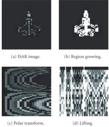
(a) ISAR image. (b) Region growing.
(c) Polar transform. (d) Lifting. Figure9: Simulation results for MIG-25.
ISAR image with the assumption that the target motion is uniform within the window duration. But this may not be true for longer window duration and hence degrades the ISAR image. Further, to capture the Doppler information effectively, better frequency resolution is required, which is achieved with longer window provided that the data available is sufficient. If sufficient amount of data is not available, then the window length should be chosen such that it provides better frequency resolution. Here, the window length of 32 is used for the computation of STFT as it provides better re-sults. Like STFT, TFR by HW also suffers from tradeoff be-tween time resolution and frequency resolution. That is, the shorter the window length, the better the frequency resolu-tion with poorer time resoluresolu-tion would be, and vice versa. This is because TFR by HW involves windowing the spec-trum instead of data as in STFT. As better frequency res-olution is required to capture the Doppler information ef-fectively, shorter window is considered while computing the TFR by HW. Further, use of rectangular window generates HW of infinite duration in time. Use of a proper smooth-ing window other than a rectangular one makes it finite in time. Considering the above arguments, hamming window of length 4 for computing the TFR by HW is found to pro-vide better results.
The reconstructed gray scale ISAR images of size 64×64 are given as input to the target recognition block. The re-sults are shown in Figures9,10,11, and12for different im-age patterns. The efficiency of the region-growing technique over edge-based technique in object extraction can be seen. The polar pattern for the rotated MIG-25 (Figure 10) and MIG-25 (Figure 9) can be compared to visualize how the polar transform converts object rotation into circular shifts for applying the FT. Wavelet transform is applied along each row (range) to get the finer level coefficients, which will help in minimizing the feature set size and thereby memory
re-(a) ISAR image. (b) Region growing.
(c) Polar transform. (d) Lifting. Figure10: Simulation results for rotated MIG-25.
(a) ISAR image. (b) Region growing.
(c) Polar transform. (d) Lifting. Figure11: Simulation results for 50% scaled MIG-25.
quirements. Further, finer level wavelet coefficients with the decimated Fourier coefficients (8×8) are taken as the feature set for classification. Back propagation network with input layer of 64 nodes, one hidden layer of 32 nodes, and output layer of 9 nodes is used for classification.
4.1. Classification results
(a) ISAR image. (b) Region growing.
(c) Polar transform. (d) Lifting. Figure12: Simulation results for B-727.
Table2: Recognition results for different scaling factors.
Percentage (%) Scaling factor
0.5 0.6 0.7 0.8 0.9 1.2
Recognition rate 93.73 97.38 98.68 100 100 100
Error rate 2.12 0.27 0 0 0 0
Rejection rate 4.15 2.35 1.32 0 0 0
results for different scaling factors are shown inTable 2. Rec-ognition rate is defined as number of targets properly identi-fied per total number of targets, error rate is defined as num-ber of targets falsely identified per total numnum-ber of targets, and rejection rate is defined as number of unknown targets per total number of targets. Classification results for diff er-ent rotation angles are not given, as the change in recognition results is nominal. As the scaling factor decreases, the extent of interpolation required in getting the feature set increases, thereby decreasing the recognition rate.
5. CONCLUSIONS
A new method of ISAR imaging based on TFR by HW is pro-posed in order toreduce the computationsinvolved in ISAR imaging. The performance of the proposed method is com-pared with CWD as well as STFT in terms of performance as well as computational complexity. Further, the proposed method provides similar/better results with significant re-duction (92%) in computations compared to that by CWD. The ISAR images obtained from the proposed method are used for target identification. For target identification, a neu-ral network-based ATI scheme is used which is invariant to translation, rotation, and scaling. Because of low SNR and poor resolution of ISAR images, region-growing technique
is used instead of conventional edge-based techniques to im-prove the accuracy in centroid calculation. The use of fea-ture set that is invariant to translation, rotation, and scaling, achieves good recognition results for all test patterns.
Abbrevations
ISAR Inverse synthetic aperture radar
RF Radio frequency
LFM Linear frequency modulation
SFM Stepped-frequency modulation
HW Harmonic wavelet
FT Fourier transform
IFT Inverse Fourier transform
STFT Short-time Fourier transform
FFT Fast Fourier transform
WVD Wigner-Ville distribution
CWD Choi-Williams distribution
TFR Time-frequency resolution
ANN Artificial neural networks
HWC Harmonic wavelet coefficients
CWT Continuous wavelet transform
AJTFT Adaptive joint time-frequency transform
AWT Adaptive wavelet transform
EAWT Evolutionary adaptive wavelet transform
ADS Adaptive spectrogram
ATI Automatic target identification
ACKNOWLEDGMENTS
The first author is grateful to Dr. S. V. Narasimhan, Deputy Director, DSP Systems Lab, National Aerospace Laborato-ries, Bangalore, India, who taught him harmonic wavelets. The authors would like to express their gratitude to the anonymous reviewers for their helpful and constructive com-ments. The authors are thankful to Mr. C. R. Patil, Mem-ber (Research Staff), Central Research Laboratory, Banga-lore, India, for reviewing and helpful comments.
REFERENCES
[1] V. C. Chen and S. Qian, “Joint time-frequency transform for radar range-Doppler imaging,”IEEE Transactions on Aerospace and Electronic Systems, vol. 34, no. 2, pp. 486–499, 1998. [2] V. C. Chen and H. Ling,Time-Frequency Transforms for Radar
Imaging and Signal Analysis, Artech House, Boston, Mass, USA, 2002.
[4] K.-T. Kim, I.-S. Choi, and H.-T. Kim, “Efficient radar tar-get classification using adaptive joint time-frequency process-ing,”IEEE Transactions on Antennas and Propagation, vol. 48, no. 12, pp. 1789–1801, 2000.
[5] V. C. Chen, “Reconstruction of inverse synthetic aperture radar image using adaptive time-frequency wavelet trans-form,” inWavelet Applications II, vol. 2491 ofProceedings of SPIE, pp. 373–386, Orlando, Fla, USA, April 1995.
[6] I.-S. Choi, B.-L. Cho, and H.-T. Kim, “ISAR motion com-pensation using evolutionary adaptive wavelet transform,”IEE Proceedings of Radar, Sonar and Navigation, vol. 150, no. 4, pp. 229–233, 2003.
[7] L. Cohen,Time-Frequency Analysis, Prentice-Hall, Englewood Cliffs, NJ, USA, 1995.
[8] L. Cohen, “Time-frequency distributions—a review,” Proceed-ings of the IEEE, vol. 77, no. 7, pp. 941–981, 1989.
[9] D. E. Newland, “Practical signal analysis: do wavelets make any difference?” inProceedings of Design Engineering Technical Conferences (DETC ’97), Sacramento, Calif, USA, September 1997.
[10] D. E. Newland, Random Vibrations, Spectral and Wavelets Analysis, Longman, Singapore, 3rd edition, 1993.
[11] D. E. Newland, “Wavelet analysis of vibration, part I: theory,” Transactions of the ASME: Journal of Vibration and Acoustics, vol. 116, no. 4, pp. 409–416, 1994.
[12] D. E. Newland, “Time-frequency and time-scale signal analysis by harmonic wavelets,” inProceedings of the 1st European Con-ference on Signal Analysis and Prediction, pp. 53–59, Prague, Czech Republic, June 1997.
[13] E. Oja, “Neural networks, principal components, and sub-spaces,”International Journal of Neural Systems, vol. 1, no. 1, pp. 61–68, 1989.
[14] P. Comon, “Independent component analysis, a new con-cept?”Signal Processing, vol. 36, no. 3, pp. 287–314, 1994. [15] A. Al-Ani and M. Deriche, “A hybrid information
maximi-sation (HIM) algorithm for optimal feature selection from multi-channel data,” inProceedings of IEEE International Con-ference on Acoustics, Speech, and Signal Processing (ICASSP ’00), vol. 6, pp. 3470–3473, Istanbul, Turkey, June 2000. [16] P. A. Devijver and J. Kittler,Pattern Recognition: A Statistical
Approach, Prentice-Hall, London, UK, 1982.
[17] S. K. Pal, “Fuzzy set theoretic measures for automatic feature evaluation: II,”Information Sciences, vol. 64, no. 1-2, pp. 165– 179, 1992.
[18] R. Battiti, “Using mutual information for selecting features in supervised neural net learning,”IEEE Transactions on Neural Networks, vol. 5, no. 4, pp. 537–550, 1994.
[19] L. M. Belue and K. W. Bauer Jr., “Determining input features for multilayer perceptrons,”Neurocomputing, vol. 7, no. 2, pp. 111–121, 1995.
[20] D. W. Ruck, S. K. Rogers, and M. Kabrisky, “Feature selec-tion using a multilayer perceptron,”Journal of Neural Network Computing, vol. 2, no. 2, pp. 40–48, 1990.
[21] P. Wunsch and A. F. Laine, “Wavelet descriptors for multires-olution recognition of handprinted characters,”Pattern Recog-nition, vol. 28, no. 8, pp. 1237–1249, 1995.
[22] I. Daubechies, Ten Lectures on Wavelets, vol. 61 of CBMS-NSF Regional Conference Series in Applied Mathematics, SIAM, Philadelphia, Pa, USA, 2nd edition, 1992.
[23] R. C. Gonzalez and R. E. Woods,Digital Image Processing, Ad-dison Wesley, Boston, Mass, USA, 1993.
[24] Y. Yokoyama, Y. Miyamoto, and M. Ohta, “Very low bit rate video coding using arbitrarily shaped region-based motion compensation,”IEEE Transactions on Circuits and Systems for Video Technology, vol. 5, no. 6, pp. 500–507, 1995.
[25] G. H. Granulund, “Fourier processing for handwritten charac-ter recognition,”IEEE Transactions on Computers, vol. 21, pp. 195–201, 1992.
B. K. Shreyamsha Kumarreceived the B.E. degree in electronics and communication engineering from Bangalore University, In-dia, in 2000. He received the M.Tech. degree in industrial electronics from National In-stitute of Technology, Karnataka, Surathkal, India, in 2004. He joined Central Research Laboratory as a Member (Research Staff) in 2004. He has two international conference papers in to his credit. His areas of research
include group delay functions, spectral estimation, time-frequency representation, inverse synthetic aperture radar imaging, wavelets and image processing.
B. Prabhakar received the B.Tech. degree in electronics and communication engi-neering from Shri Venkateswara University, Tirupati, India, in 1997, and continued as a Faculty Member for one year. He received the M.Tech degree in digital signal pro-cessing from Indian Institute of Technol-ogy, Kanpur, India, in 2000. He joined Cen-tral Research Laboratory as a Member (Re-search Staff) in 2000. He has more than 10
research papers in international as well as national conferences. His research activities include image compression, video compression, tracking and pattern recognition.
K. Suryanarayanareceived the B.Tech. de-gree from Mangalore University, India, in 1998. He received the M.Tech. degree in system analysis and computer application from Karnataka Regional Engineering Col-lege, Surathkal, India, in 2001. He joined Central Research Laboratory as a Member (Research Staff) in 2001. He has more than five research papers in international as well as national conferences. His research
activ-ities include radar imaging, multitarget tracking and radar signal processing.
R. Rajagopalgraduated from Madras Uni-versity with B.E. (Honors) in 1982. He got his M.E. and Ph.D. degrees from Bharathidasan University, Tiruchirappalli. He worked in the Regional Engineering College, Trichy, in various capacities from 1982–1998. He joined Central Research Laboratory, Bangalore, in June 1998. He is currently Head of Radar Signal Processing Group. He has published more than 50