Optimization of Radiators, Underfloor and Ceiling Heater Towards the Definition of a Reference Ideal Heater for Energy Efficient Buildings

Optimization of radiators, underfloor and ceiling

heater towards the definition of a reference ideal

heater for energy efficient buildings

Andrea Ferrantelli1,* , Karl-Villem Võsa1and Jarek Kurnitski1,2

1 _{Tallinn University of Technology, Department of Civil Engineering and Architecture, Ehitajate tee 5, 19086}

Tallinn, Estonia; [email protected] (A.F.); [email protected] (K-V.V.) 2 _{Aalto University, Department of Civil Engineering, P.O.Box 12100, 00076 Aalto, Finland;}

[email protected] (J.K.)

* Correspondence: [email protected]

Abstract: Heat emitters, as the primary devices used in space heating, cover a fundamental role in the energy efficient use of buildings. In the search for an optimized design, heating devices should be compared with a benchmark emitter with maximum heat emission efficiency. However, such an ideal heater still needs to be defined. In this paper we perform an analysis of heat transfer in a European reference room, considering surface effects of thermal radiation and computing the induced operative temperature (op.t.) both analytically and numerically. Our ideal heater is the one determining the highest op.t. By means of functional optimization, we analyse trends such as the variation of operative temperature with radiator panel dimensions, finding optimal configurations. In order to make our definitions as general as possible, we address panel radiators, convectors, underfloor (UFH) and ceiling heater. We obtain analytical formulas for the operative temperature induced by panel radiators and identify the 10-type as our ideal radiator, while the UFH provides the best performance overall. Regarding specifically UFH and ceiling heaters, we find optimal sizes providing maximum op.t. The analytical method and qualitative results reported in this paper can be generalized and adopted in most studies concerning the efficiency of different heat emitter types in building enclosures.

Keywords: radiator efficiency; energy; operative temperature; analytical model; computer simulations

1. Introduction

The energy performance of heat emitters is a key factor in the energy demand of the building sector, which is primarily determined by space heating [1–3]. Such devices can be of very different type (panel radiators, convectors, ceiling and underfloor heating...), each determining the energy demand in a specific way [4–8]. For these reasons, several studies have investigated the emitters’ performance on both the experimental and theoretical viewpoint [9–11], focusing especially on the design, specific type and room placement of panel radiators (e.g. close to a window or slightly detached from a wall) [4,12–18]. For instance, measurements have shown a better performance of low temperature panel radiators [19], and a sensibly different outcome for serial and parallel connected radiators [9].

Despite such recent advances, this kind of investigation seems to be very involved, for a variety of reasons. Contrasting results also exist: an experimental investigation of a convector, a radiant and a baseboard heater showed a lower energy consumption by the convector [7], in contrast with the classic work by Olesen et al. [4], written in the early 80s. While it was concluded in [7] that the cause was probably the improved flow outlet design of the newer convector, an older study already considering this improvement [13] agreed instead with [4].

Previous research regarding the energy performance of heat emitters has largely dealt with matters of emission efficiency and losses within the system. In such a framework, one typically addresses the emitted power and energy usage by the system under predefined boundary conditions [20,21]. So

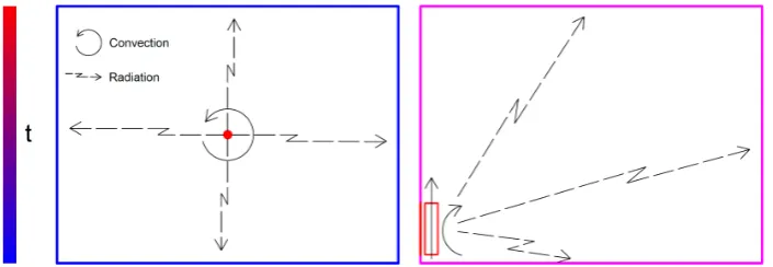
Figure 1.Ideal point heater (left) and real heat emitter (right).

far, this approach has been effective enough for product characterisation. However, the methodology fails to take into account the different levels of thermal comfort provided by the heaters at equal air temperature (which is the target value that is kept constant throughout product comparison). Such a difference in the thermal environment can affect negatively even the perceived productivity in the workplace, with a seizable economical impact [22,23]. More importantly, accounting for this phenomenon could allow for some direct energy savings if different set-points within the heating systems could be used.

Thermal comfort within an enclosure can be quantified with the so-called operative temperature (hereinafter op.t. ortop), which is finding an increasing use recently [9,13,18,24]. This is defined as the uniform temperature of an enclosure in which an occupant would exchange the same amount of heat by radiation and convection as in the existing non-uniform environment [25].

Unfortunately, such a formulation generates a fundamental problem for product comparison, as it does not provide one clear "ideal" emitter to benchmark others against. For ordinary systems where the air temperature is controlled, such an ideal heater is generally described as a dimensionless point (Figure1). Heat is transferred by convection to the thermal node of indoor air, and by radiation to the surrounding surfaces. A higher convective transfer fraction induces lower surface temperatures on the surrounding surfaces with minimal heat loss, as in Fig.1. To reach the desired air temperature set-point tair, an emitter with convective fraction of 1 (pure convection) thus requires the lowest possible heat output. In this sense, it represents an "ideal" heater.

By the definition of operative temperature however, top is inversely proportional to the surrounding surfaces’ temperatures. In this respect, the "ideal" device described above should now exhibit a lower performance, as it heats the surrounding surfaces only minimally. As we will illustrate in the following, preliminary simulations with the software IDA ICE [26] confirm indeed that a number of real emitter configurations can outperform the point heater (or convector). In other words, defining an ideal benchmark heater for operative temperature control is non-trivial, and needs to be addressed for better comparison between different heat emitter systems.

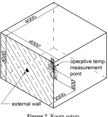
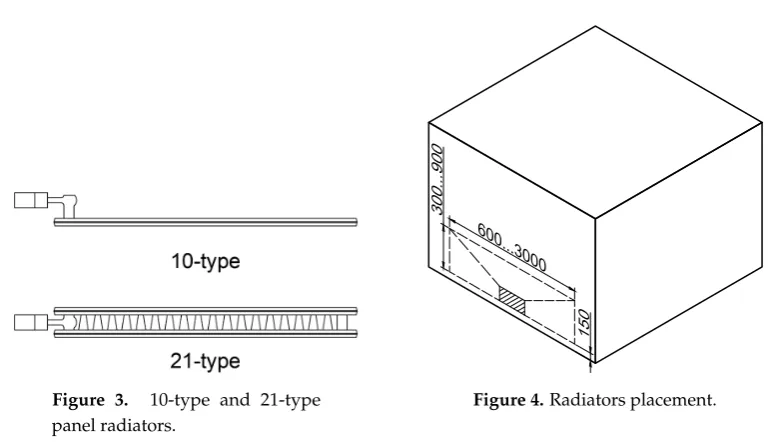
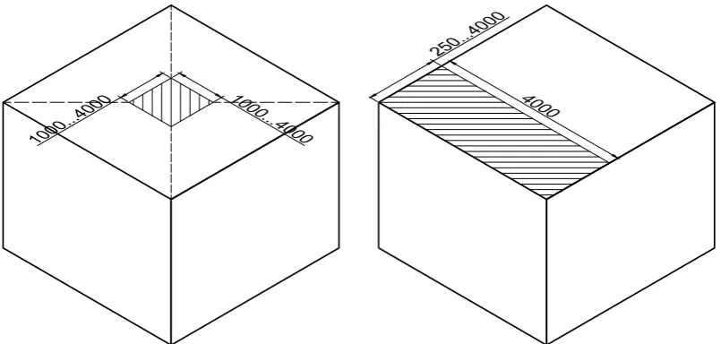
To this aim, in the present paper we consider an average-sized enclosure provided by the CEN technical committee TC130 working group WG13, with a user sitting in the middle (Figure2). We investigate how the operative temperature sensed by this user changes with the typology and size of emitter, and whether there exist optimal configurations corresponding to the highesttop. We address panel radiators (10- and 21-type), underfloor (UFH) square, UFH strip and ceiling heater. A 10-type radiator has only one panel and no convector fins, while the 21-type has two panels with one set of fins in between, as illustrated in Fig.3. They are placed on the cold wall, with centrelines aligned, as in Fig.4.

Figure 2.Room setup.

as a function of the emitters’ dimensions to identify general trends, comparing the different devices and finding optimal configurations.

Concerning panel radiators, by keeping the heat output constant we determine analyticaltop curves in function of their panel dimensions, finding an optimal width range of both the 10- and 21-type. We prove that the thermal comfort performance of radiators is more sensitive to the height than to the width, and that the convector and 21-type provide the lowest operative temperatures. On the other hand, the 10-type can provide atopas high as the air temperature, and accordingly it can be identified as our "ideal" emitter. For the case at hand, we also list a series of analytical formulas for calculatingtopfor radiators of 10- or 21-type, with panel size in the range considered and excluding back wall losses1.

The UFH and ceiling heater provide in general higher operative temperatures, approaching, and often exceeding, the air temperature. We find, both analytically and numerically, a maximumtopfor sizes smaller than the whole width of the room: the analytical solution allows to locate them precisely, up to three digits. Remarkably, if one considers typical radiator sizes with height 0.6m, when compared to a 10-type the UFH provides atop that is higher by 0.25 K - 0.3 K, and by 0.35 K in the case of a 21-type2.

The present paper is organized as follows: in Section 2 we describe the test chamber, the simulation setup and the different methods for computing the operative temperature. In Section 3we report our results for each single case, some general discussion then appears in Section4and finally, Section5contains a summary of our findings and concluding remarks. In the Appendix we include considerations about the view factors, a comparison between our analytical and numerical methods and the analytical formulas to determine the operative temperature for any radiator size discussed in the study.

2. Method

In this study, we consider an enclosure with thermal layer properties and dimensions 4mx4mx3m specified by the CEN TC130 European Committee, shown in Figure2. The external wall has U-value

1 _{Adiabatic internal surfaces are used in the model, namely no additional heat is transferred from the ceiling heater and UFH} to the colder rooms above and below. This additional heat loss is also omitted for the radiators, to guarantee an accurate comparison.

Figure 3. 10-type and 21-type panel radiators.

300...900

600...3000

150

Figure 4.Radiators placement.

0.25 W/m2K, and heat recovery ventilation in the room provided an air change rate of 1 ACH with temperature efficiency 0.8.

Vertical temperature gradients are mainly influenced by the amount of air circulation within an enclosure. As it was shown in [8], gradients measured for radiators and UFH were approximately 0 K/m for ventilated rooms. The ventilation flow rates and room geometry (mainly the height of the room) within the referenced study are similar to the room considered in this paper. We accordingly neglect the possible effects of a vertical temperature gradient, assuming indoor air mixing and lack of stratification to be similar. This approximation is therefore true at least for radiators and UFH, however no information exists for ceiling heater. We do note that including a vertical gradient would yield marginally different surface (and thus operative) temperatures, since the temperature differences for convection calculation purposes would change between the room air and enclosing surfaces only slightly. A more detailed study on this phenomenon would certainly be interesting, however it would require extensive measurements to accurately assess the variation in the gradient values, as the size of the emitters changes within a broad range.

We locate the calculation point, namely the centre of mass of an average sitting user, at 0.6m above the floor in the room centre (i.e., at 2m distance from each wall) [25]. The most performing heater configuration will then be the one providing the highest operative temperature, with the same heater nominal output. The steady-state boundary conditions are the following: Indoor air temperature Tin=20 °C, external air temperatureText= -15°C. Both direct normal and diffuse horizontal irradiance are set to zero. 134 W of power are required to heat up the room under these predefined conditions (the heat outputs throughout the simulations were within±0.5 W of this value).

IDA-ICE calculates the heat emission from any hydronic heating device as follows. The characteristic equation used to determine and model the device’s heat output comes in the form of an empirical power law [21],

P=kldTn, (1)

wherekandnare coefficients determined individually for each emitter type, withlits length anddT the logarithmic mean temperature difference between heating water and indoor air. This governing equation therefore holds true for radiators, ceiling panels and UFH. The detailed version of the model, containing the heat balance equations used in the IDA ICE software for e.g. the calculation of relevant flow and surface temperatures, can be found in [28].

for the underfloor heating system. The maximal mass flowGmaxthrough the underfloor piping is then calculated as

Gmax= _∆TPnom

nomcp, (2)

wherecpis the specific heat capacity of water at constant pressure. The exact heat output, return temperature and mass flow depend on the actual amount of heat required within the room.

Heat transfer from the heating water to the surfaces of heating pipe and floor is modelled with an n-layered RC-network, see [28] for exact model descriptions. The piping layer is basically given by a heat exchanger, with an active plane at constant surface temperature located inside the floor slab. In the resulting floor coil model, the heat transfer between fluid and active plane is computed via their logarithmic temperature difference; the according heat transfer coefficient includes convection between medium and tube wall, heat conduction through the tube walls and "fin efficiency" given by the distance between immersed tubes or actual fins. In steady state, this approach corresponds to the resistance method of the EN 15377-1 standard [29].

For a selection of IDA ICE model and software validations, see e.g. [30–34].

The operative temperaturetopis computed analytically, according to the prescriptions of the ISO 7726 standard, as we explain in the following. Considering the contributions of all the six surfaces in the enclosure, we obtain an expression fortop=top(a,b)that is a function of the radiator heighta and widthb. The eventual global maxima of this function in the(a,b)plane would then correspond to the optimal configuration for that specific heater. Such full analytical solution is then numerically validated by the finite difference method software IDA ICE [26] in the same CEN TC130 test room, in the limit when only the contribution of the surfaces that are parallel to the principal calculation surface is accounted for.

The operative temperature at the above location is not uniquely defined. In IDA ICE this is evaluated as the simple arithmetic average of air temperaturetairand mean radiant temp. ¯tr [26],

top= tair

+¯tr

2 , (3)

(throughout this paper, [ti]=[°C ] and [Ti]=[K]). This differs from the exact definition given in the ISO 7726 [25],

top= hctair

+hrt¯r hc+hr

≡Atair+ (1−A)t¯r, (4) where the average is weighted by the radiation and convection heat transfer coefficientshrandhcat the calculation point3. The explicit formula for the coefficientA, which is itself a function ofhcandhr, is given in the Appendix; for our setup, it lies within the rangeA∼0.5−0.6.

Another difference between the ISO standard and IDA ICE is that the numerical software has a peculiar way of computing the mean radiant temperature ¯tr. It considers only the surfaces that are parallelto the principal calculation surface, therefore the sum of view factors in a principal direction is<1 (Figure5). Moreover, ¯tris obtained as the average of mean radiant temperatures from the six principal directions, weighted by the respective view factors,

Tmrt= 4

v u u t

∑6

i=1∑nj=1Fi→jTj4 ∑6

i=1∑nj=1Fi→j

, (5)

where theFi→jare computed for a small area (the observer) that is only parallel to the radiating surface.

Figure 5. Calculation of mean radiant temperature from IDA-ICE [26].

Figure 6. Calculation of mean radiant temperature from ISO 7726 [25].

In contrast, the ISO 7726 prescribes that for each direction one considers both paralleland perpendicular surfaces (see Figure6), obtaining the plane radiant temperature [14,25],

T(pri)= 4

v u u t

6

∑

j=1

Fp−A_jT_sj(i)4, (6)

with the angle factorsFp−Ajreported in the Appendix. Now the sum of view factors in each direction is accordingly =1, and the mean radiant temperature is given by [25],

¯

tr(a,b,c) = 4

v u u

t∑

6 i=1βiT

(i) pr(a,b,c) ∑6

i=1βi

−273.15, (7)

namely by a weighted average over the projected area factorsβiof a person, listed in Table1.

Table 1.Projected area factors of a person [25].

Standing Seated

Up/down 0.08 0.18

Left/right 0.23 0.22 Front/back 0.35 0.30

Specifically, in this work all the "Analytical Full"top points in the graphs are calculated with Eqs.(4) and (7), therefore following the ISO standard completely throughout this paper. The only point in common with IDA ICE consists of the surface temperaturesT_sj(i), which are written as polynomial interpolations from the data provided by the software. Since both the definitions of operative and mean radiantTare different, the analyticaltopis independent of the numericaltop.

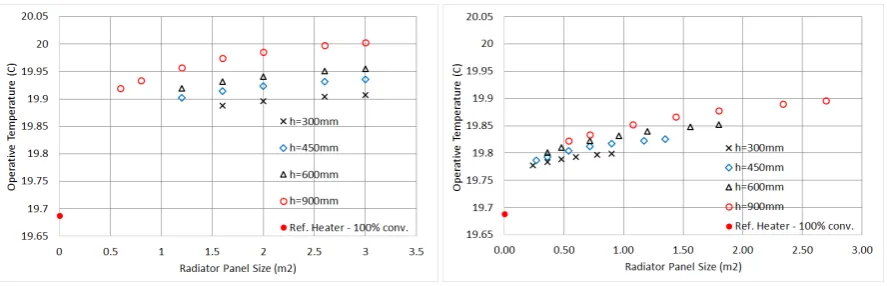
Figure 7.IDA ICE operative temperatures for a 10-type radiator and convector in function of the panel area.

Figure 8.IDA ICE operative temperatures for a 21-type radiator and convector in function of the panel area.

The "strip" configuration instead considers a heated strip running from the cold (or external) wall. Further descriptions are given in Sections3.2and3.3.

3. Results

3.1. Panel radiator

As discussed in the previous section, in this study we consider a room with a single external wall and adiabatic internal walls, floor and ceiling under steady-state conditions. Thermal layer properties and room dimensions (Figure2) are chosen according to the European CEN technical committee TC130 working group WG13 specifications, with a U-value for the external wallU=0.25 W/m2K. A supply temperature of 55°C was used. Different types and sizes of heat emitters (radiators, UFH and ceiling heater) are used in IDA ICE simulations to offset the heat loss through the external wall (specific details for each emitter type are presented in their relevant sections). The resulting surface temperatures as calculated by the software are logged and used as input in the analytical calculation. The operative temperatures computed by IDA ICE are also used for comparison with the analytical result.

Figures7and8illustrate first of all that the area by itself is not a good parameter for assessing the performance related to the operative temperature: given the same area, the efficiency varies with height. Additionally, and more importantly, we observe that one cannot identify a reference ideal convector with 100% convection and 0% radiation as an ideal heater, since it returns the lowesttop.

Operative temperatures for fixed heights are plotted in Figures9and10. These hold respectively for a 10-type and a 21-type panel radiator (some values for the 10-type are missing, as it could not reach 134W of power output). One can see that in general, the numerical and analytical solutions are nearly equivalent. Only for the 10-type we see a slight deviation; moreover, the 10-type reveals to be the most performing radiator, withtopvalues always exceeding those of the 21-type by∼0.1°C . They can even approach the air temperature 20°C ath=0.9m. We can thus conclude that for the study at hand the 10-type can be identified as our "ideal" radiator.

Further conclusions can be made rigorous by means of our analytical solution. First of all, the topvalues are linearly distributed along different heightsh. By applying a method first introduced in [27], we interpolate the operative temperature versus the height (minimum square method), for a fixed width. The according curves can be generally written as

Figure 9. Operative temperatures for a 10-type panel radiator, with h=0.3, 0.45, 0.6, 0.9m.

Figure 10. Operative temperatures for a 21-type panel radiator, with h=0.3, 0.45, 0.6, 0.9m.

In contrast, assuming a given height providestopvalues that arenotlinearly distributed along different widthsw. They rather follow a quadratic law in the form

top(h,w) =A(h)w2+B(h)w+C(h). (9) As it is shown in TablesA3andA4, one finds A(h) < 0 for any height. topgrows instead linearly with increasing height,top(h,w) =A(w)h+B(w)withA(w)>0 (TablesA1andA2): this verifies the physical result that the operative temperature is more dependent on the height than on the width4_.

The analytical solution allows to make even more specific conclusions. As an example, consider the 21-type radiator. The explicit form of the operative temperature is generally highly non linear, however plotting the first derivative Dtop ≡ dtop/dwin function of the width returns additional information. In Figure11we find indeed a "plateau" starting atw ∼1m and ending at about 2m, where the decrease withwis less pronounced: in other words, in the according range∆wthe operative temperaturetopis optimised with respect to width increase, and widths contained in this interval are most advantageous.

The approximated range∆wabove is probably precise enough for practical applications, however an analytical formula such as Eq.(9) allows to identify its boundaries with high precision. The second and third derivativesD2top≡d2top/dw2andD3top≡d3top/dw3provide indeed the exact locations of the plateau, atw=0.87m andw=1.86m respectively . The latter point corresponds to a minimum of D3_t

op, which identifies a change of concavity inD2top. Finally, the second derivative gives the exact point of minimal increment oftop, sitting atw=2.736m. Interestingly, exactly the same value holds forh=0.9m, as illustrated in Figure12.

To summarize, investigating the performance with respect to the induced operative temperature of 10- and 21-type panel radiators, we have rigorously proven that

• given the same area, the efficiency varies with height,

• an ideal convector with 100% convection performs worse than panel radiators, • the 10-type can be identified as our ideal heater,

• the operative temperature is more dependent on the height than on the width, • there exists an ideal width range for 21-type radiators.

Figure 11. First derivative of the analytical operative temperature for a 21-type radiator, h=0.3m.

Figure 12. First derivative of the analytical operative temperature for a 21-type radiator, h=0.9m.

1750...4000

1750...4000

Figure 13.Underfloor heating - square setup

4000

750...4000

Figure 14. Underfloor heating - strip setup

Furthermore, we provide in TablesA1toA4useful analytical formulas which determine precisely the operative temperatures for any width and height in the ranges considered in the study at hand.

3.2. Underfloor heating

Regarding underfloor heating (UFH), we considered two different cases: a square heater in the centre of the floor, with varying side length (Figure13), and a strip setup with fixed width as the floor and varying depth from the external wall (Figure14). A nominal heat output of 50 W/m2 at a water-side temperature drop of∆T=7Kwas used as input for the IDA ICE model, with the piping

placed at 25mm depth in screed. A 30 W/m2K fluid-to-slab heat transfer coefficient and a supply temperature of 35°C were used.

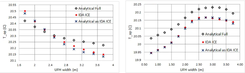
The operative temperature for square and strip UFH is plotted in Figs.15and16respectively. Here we compare IDA ICE (dots) with an analogous analytical calculation with no projection on perpendicular surfaces (crosses) and with the full analytical calculation (all the 6 directions with perpendicular surfaces), diamonds.

Figure 15.Operative temperature for a square UFH.

Figure 16.Operative temperature for a strip UFH.

width is around 2m: considering the horizontal and vertical walls as a whole, this case corresponds to the most symmetric configuration indeed. As it can be seen by investigating the view factors of each surface, for smaller squaresw<2m IDA ICE does not account for the heat dissipation to the vertical walls5. On the other hand, forw>2m these contribute to increasingtopat the calculation point (2m from each wall, at 0.6m from the floor). The main result in any case is that there is no evident optimal size for the UFH with this configuration.

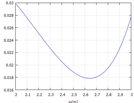
In the case of UFH as a strip running between the side walls, starting from the cold wall, we find instead something more interesting. Neglecting the vertical walls we get again an excellent cross-check with IDA ICE; furthermore, the extension to the full enclosure shows a systematic difference of nearly 0.1°C, accounting for the effect of vertical walls. While qualitatively there is basically no deviation from the numerical solution, this is interesting when considering precision calculations.

More importantly, we find a very distinct maximum fortopbetween 3m and 3.1m, Figure16. By means of the analytical form of the solution, we can compute its location precisely atw=3.0372m, see Fig.21. Notice also that, qualitatively, the operative temperature difference between radiators and a fully covering UFH is comparable to that obtained in the experimental paper [8].

3.3. Ceiling heater

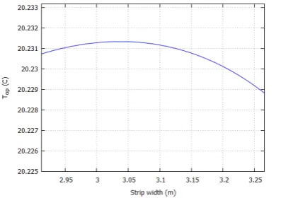
The two configurations of square and strip heaters we addressed for floor heating were also considered for the ceiling (Figures17and18). Geometrically, the setup is a mirror-reflection of the floor model on the vertical axis. The main difference in the view factors is in the calculation point, which now sits at 2.4m from the heated surface, making the reflection not perfectly symmetrical. Catalogue values of a well-known manufacturer were applied for the IDA ICE model input (nominal heat output of 529.2W/m2at∆Tln =50Kwith characteristic exponent n=1.174). A supply temperature of 45°C was used. The operative temperatures in this case are given in Figures19and20, and the absolute maximum for a heated strip is shown in Fig.22. It occurs atx=3.1349m.

Comparing Figure19with Fig.15, we notice a marginal difference forw<2m, while otherwise the same highertopwith respect to IDA ICE is obtained. The operative temperature values are naturally smaller in this case, due to the larger distance heater-observer that reduces the heat transfer. For a heated strip, this is reflected in Figure20, showing a smaller effect of the vertical walls compared to Figure16. Qualitative differences are irrelevant.

1000...4000

1000...4000

Figure 17.Ceiling panel - square setup

4000

250...4000

Figure 18.Ceiling panel - strip setup

Figure 19.Operative temperature for a heated square portion of the ceiling.

Figure 20.Operative temperature for a heated strip on the ceiling.

4. Discussion

Besides a number of specific results, in this paper we have shown quantitatively two general features: how the radiator performance for thermal comfort changes with panel area, and the existence of optimal sizes for the UFH and ceiling heater.

These findings are supported by well-tested approaches such as the view factors (see e.g. the standard [25]), which constitute the foundation of our analysis. In this respect, the analytical calculation is necessary for two main reasons: first, IDA ICE calculates the operative temperature in a very specific way that is different from the ISO prescription6_{. Since we are aiming to contribute to the heat emission} code EN 15316-2-1:200, a more standard procedure is preferable.

Secondly, and more importantly, we are able to extrapolate and generalize our results toany 10- or 21-type emitter with size included in the studied range, by virtue of the simple interpolation method introduced in [27]. The exact formulas listed in TablesA1toA4can be of practical use for qualitative assessments of thermal comfort induced by radiators of 10- or 21-type, with dimensions 0.3m≤h≤0.9mand 1.2m≤w≤3mand assuming no back wall losses.

In our simulation setup, temperature limits for the water supplied to the emitters are imposed on their systems for a variety of reasons. In theory, any size of emitter in any configuration could be used to offset the heat loss through the external wall, with smaller devices needing hotter surfaces (thus requiring a higher supply water temperature). However, practical reasons bound these temperatures

6 _{As we have shown, thet}

Figure 21. Operative temperature maximum for a strip heated area underfloor.

Figure 22. Operative temperature maximum for a heated strip on the ceiling.

greatly. For example, floor surfaces with UFH in living rooms are limited to 27/29 °C to avoid thermal discomfort [35]. Moreover, large surface temperature differences in opposing directions can cause local discomfort via a phenomena called "radiant temperature asymmetry" [25]. In addition, supply water at low temperature can be generated by ground and air source heat pumps with a higher thermal efficiency. Finally, warmer supply water would also yield higher embedded losses.

It should be also noted that if a UFH heated square could follow and track an occupant location, this solution would represent the best performing heater with the highest operative temperature, a result that may have practical implications for personal thermal comfort solutions7.

As the differential between outdoor and indoor air temperature decreases, we expect the corresponding∆t=tair−topto do the same, since each and every wall surface temperature tends to approachtair. The emitters’ surface temperatures will decrease as well, affecting ¯trand therefore topaccordingly. In other words, for a more realistic (higher) outdoor temperature we expect∆tto be generally smaller than what reported in this study. The surface temperatures for our enclosure are listed in Table2for the smallest size of each emitter type addressed in this study.

The occurrence of a maximumtopfor UFH and ceiling heater strips that do not cover the floor or ceiling entirely implies that the remaining area does not contribute to thermal comfort, which might be interesting for energy saving purposes. More generally, the finding thattopapproaches in some cases tairis very advantageous for energy saving, as it was shown e.g. in [36] that the energy demand is very sensitive to operative temperature corrections. In particular, a difference of only 0.1°C can increase the annual heating need by 1-2% [36]: such effect is found for both the convector and the 21-type panel radiator, which are therefore fairly underperforming.

All these results are obtained by a rather general methodology. Our model can easily be extended to any study where it is possible to express the quantity of interest in function of the system variables: in the case of HVAC for instance, one could investigate how the indoortair changes according to different inlet velocities and/or temperatures, to the diffusers and windows location and so on.

5. Conclusions

In this paper we have compared quantitatively the operative temperature induced by different types of heat emitters, in the search for the most performing, or "ideal", heater for thermal comfort. We considered a number of configurations of practical interest, with analytical and numerical calculations oftopperformed in a test room with a standard size defined by updated European Standards.

Table 2.Emitter and room surface temperatures [°C] for minimal sized emitters.

Emitter type Emitter surf. Floor Ceiling Sidewalls Backwall External wall

10-type radiator 33.83 19.78 19.80 19.72 19.74 18.59

21-type radiator 32.04 19.61 19.71 19.60 19.62 18.53

UFH, square 24.66 19.89 20.03 20.01 20.03 18.92

Ceiling heater, square 31.78 20.00 19.90 19.95 19.96 18.87

We first addressed panel radiators of 10- and 21-type installed on the cold wall, for a variety of sizes and surface temperatures. Compared with an ideal convector providing the same output∼134W, we found the 10-type to be the most performing radiator, and accordingly the "ideal" radiator for the setup considered in this paper. By means of our analytical calculations, we were able to draw a number of considerations, proving for instance that the thermal comfort performance of radiators is more sensitive to the height than to the width.

For underfloor UFH and ceiling heater strips, we identified the occurrence of non-trivial global maxima, corresponding to the highest temperature sensed by a person sitting in the middle of the room. Furthermore, compared to typical radiator sizes with height 0.6m, the UFH provides 0.25 K - 0.3 K highertoprelative to the 10-type and 0.35 K relative to the 21-type. In general, we found the convector and the 21-type panel radiator to be fairly underperforming. Specifically, the former shows the worst performance: the op.temp. is lower by 0.55 K when compared to UFH. Let us remark anyway that the air and operative temperature differences calculated in this study should not be directly applied for energy saving assessment, because they are valid at the outdoor temperature -15°C, which is much lower than the average heating season value.

In conclusion, the investigation presented in this paper constitutes a good starting point for a number of improvements in the search for an ideal heater. Here we have addressed the operative temperature as the sole parameter that is responsible for thermal comfort; we therefore do not claim by any means to have provided an ultimate method for determining an ideal heater. Taken as a whole, the phenomenology of heat transfer and thermal comfort inside an enclosure depends indeed on a number of factors that are very difficult to track simultaneously.

For these reasons, there definitely exists some ground for future work. As remarked in the Introduction, our method can be easily applied to HVAC as a way to fine-tune the room ventilation. Also, we can investigate how any quantity of interest (such as the op.t.) is affected by e.g. the emitters position, the location and size of the windows, the emissivity of materials and so on. Furthermore, parametric studies on the relationship between view factors, room and geometry of the emitter might show a more general pattern, whose impact on the whole energy demand could be quantified with e.g. annual simulations.

Funding:The research was supported by the Estonian Research Council with Institutional research funding grant IUT1-15. The authors are also grateful to the Estonian Centre of Excellence in Zero Energy and Resource Efficient Smart Buildings and Districts, ZEBE, grant 2014-2020.4.01.15-0016 funded by the European Regional Development Fund.

Conflicts of Interest:The authors declare no conflict of interest.

Appendix View factors and operative temperature formulas

The view factors for a small area parallel or perpendicular to a surface of heightaand widthb, separated by a distancec, hold respectively as [25]

Fp−Ai = 1 2π

_X

√

1+X2arctan Y √

1+X2 + (X↔Y)

Figure A1. Comparison of surface temperatures for a 21-type radiator,h=

0.9m. IDA ICE (crosses) vs 4th order polynomial interpolation (diamonds).

Figure A2.Operative temperatures for a 21-type, IDA ICE cross-check: arithmetic (crosses) vs weighted average for different clothing surface temperatures.

withX=a/c,Y=b/c, and

Fp−Ai = 1 2π

arctan1 Y−

Y √

X2_+Y2arctan 1 √

X2_+Y2

, (A2)

withX=a/b,Y=c/b. We should remark that the calculation of mean radiant temperatures for the perpendicular surfaces is extremely sensitive to how the above view factors are implemented. For example, in Section3.1we discussed panel radiators of varying heighththat are installed on the cold wall, at 15cm from the floor. In this case, one could naively compute the view factor from the lower edge of the cold wall up to the top of the radiator (a=h+15cm), or alternatively ignoring the 15cm displacement (a=h). It can be shown that the view factor differs critically for both cases and returns a non physical result for the operative temperature.

The reason is that the above functions are not linear ina,b,c: since the view factors are additive, a more correct way to calculate them with formulas (A1) and (A2) consists of subtractingFp−Ai ata=h fromFp−Ai ata= h+15cm. This way one obtains anetview factor, which despite not being 100% accurate, returns physical operative temperatures that match earlier results [24,36] and the present numerical simulations (see e.g. Figs.19and20).

We conclude with a few considerations about the definition of operative temperature adopted in this paper. In Section2we remarked that IDA ICE uses the simple arithmetic average of air temperature tairand mean radiant temperature ¯tr, Eq.(3). On the other hand, for the analytical calculation we used the exact formula for computing the op.t., Eq.(4). The Acoefficient is expanded as

A≡

1+hr

hc

−1

, (A3)

and we expresshc andhr in function of the air and mean radiant temperatures by means of the following [37–39]: the heat transfer coefficient for radiation is written as

hr =σe_cl Ar

AD

(tcl+273.15)4−(¯tr+273.15)4

tcl−t¯r , (A4)

whereeclis the emissivity of a clothed person andAr/ADthe ratio of the body radiation area (0.67 for crouching, 0.7 for sitting and 0.73 for standing).e_cllies typically in the range 0.8-0.9 [40], here we use ecl=0.9. It can be shown that a 0.1 difference in the emissivity is marginal to the operative temperature, inducing anO(0.001)difference intop, which is less than 0.1%. The same holds for the ratioAr/AD, as it is evident from Eq.(A4); in this paper we chooseAr/AD=0.7. σ=5.67×10−8W/(K4m2) is the

The convection coefficient holds instead as

hc=2.384

p

tcl−tair, (A5)

if 2.38√4 _t

cl−tair >12.1 √

Vair, otherwise

hc=12.1

p

Vair, (A6)

withVair[m/s] the air velocity relative to the human body. Since for our room the air ventilation rate is 1 ACH,Vairis very small, ofO(0.01)m/s, therefore we use Eq.(A5).

The clothing surface temperature for a sitting person doing office work can vary depending on the clothing; moreover, the exact calculation is rather involved and based on a recursive formula [39]. Considering three casestcl=23, 25, 31°C, which are shown in FigureA2, one can see a small impact of tclontop. In particular,tcl=25°C reproduces the IDA ICE values almost exactly.

The operative temperature evaluated (ideally) on the surface of a clothed user is thus a function of air and mean radiant temperatures, and of the heat transfer coefficients measured at that same point. As ¯tr =t¯r(a,b,c), also the radiation coefficienthrin (A4) is a function of the radiator dimensionsaand b, together with the distance radiator-personc.

Comparison of the operative temperature as computed with (4), namely withhrandhcinstead of the arithmetic average (3) fortcl=25°C is illustrated in Fig.A3.

It can be easily verified that for underfloor and ceiling heater thetopdifference is even more negligible (of the order∼0.01°C). FigureA1also shows the precision of the interpolations used in this paper for a type-21 panel radiator.

One might also wonder about the effect of (4) on the cross-check with IDA ICE, namely when computing the mean radiant temperature without considering the heater projections on the perpendicular surfaces. The result is given in FigureA2.

Figure A3.Operative temperatures for a 21-type panel radiator, arithmetic average Eq.(3) vs average weighted with convection and radiation coefficients (A-factor in Eq.(4)).

References

1. Serrano, S.; Ürge Vorsatz, D.; Barreneche, C.; Palacios, A.; Cabeza, L.F. Heating and cooling energy trends and drivers in Europe.Energy2017,119, 425 – 434. doi:https://doi.org/10.1016/j.energy.2016.12.080. 2. D’Agostino, D.; Cuniberti, B.; Bertoldi, P. Data on European non-residential buildings. Data in Brief2017,

14, 759 – 762. doi:https://doi.org/10.1016/j.dib.2017.08.043.

3. Yao, R.; Steemers, K. A method of formulating energy load profile for domestic buildings in the UK.Energy and Buildings2005,37, 663 – 671. doi:http://dx.doi.org/10.1016/j.enbuild.2004.09.007.

4. Olesen, B.W.; Mortensen, E.; Thorshauge, J.; Berg-Munch, B. Thermal comfort in a room heated by different methods. ASHRAE transactions1980,86, 34–48.

5. Inard, C.; Meslem, A.; Depecker, P. Energy consumption and thermal comfort in dwelling-cells: A zonal-model approach. Building and Environment 1998, 33, 279 – 291. doi:https://doi.org/10.1016/S0360-1323(97)00074-7.

6. Olesen, B.W.; de Carli, M. Calculation of the yearly energy performance of heating systems based on the European Building Energy Directive and related CEN standards. Energy and Buildings2011,43, 1040 – 1050. Tackling building energy consumption challenges - Special Issue of ISHVAC 2009, Nanjing, China, doi:https://doi.org/10.1016/j.enbuild.2010.10.009.

7. Léger, J.; Rousse, D.R.; Borgne, K.L.; Lassue, S. Comparing electric heating systems at equal thermal comfort: An experimental investigation. Building and Environment 2018, 128, 161 – 169. doi:https://doi.org/10.1016/j.buildenv.2017.11.035.

8. Maivel, M.; Ferrantelli, A.; Kurnitski, J. Experimental determination of radiator, underfloor and air heating emission losses due to stratification and operative temperature variations. Energy and Buildings2018, 166, 220 – 228. doi:https://doi.org/10.1016/j.enbuild.2018.01.061.

9. Võsa, K.V.; Ferrantelli, A.; Kull, T.M.; Kurnitski, J. Experimental analysis of emission efficiency of parallel and serial connected radiators in EN442 test chamber. Applied Thermal Engineering2018,132, 531 – 544. doi:https://doi.org/10.1016/j.applthermaleng.2017.12.109.

10. Myhren, J.A.; Holmberg, S. Performance evaluation of ventilation radiators.Applied Thermal Engineering 2013,51, 315 – 324. doi:https://doi.org/10.1016/j.applthermaleng.2012.08.030.

11. Risberg, D.; Risberg, M.; Westerlund, L. CFD modelling of radiators in buildings with user-defined wall functions. Applied Thermal Engineering 2016, 94, 266 – 273. doi:https://doi.org/10.1016/j.applthermaleng.2015.10.134.

13. Ali, A.H.H.; Gaber Morsy, M. Energy efficiency and indoor thermal perception: a comparative study between radiant panel and portable convective heaters. Energy Efficiency2010, 3, 283–301. doi:10.1007/s12053-010-9077-3.

14. Kalmár, F.; Kalmár, T. Interrelation between mean radiant temperature and room geometry. Energy and Buildings2012,55, 414 – 421. doi:https://doi.org/10.1016/j.enbuild.2012.08.025.

15. Shati, A.; Blakey, S.; Beck, S. The effect of surface roughness and emissivity on radiator output. Energy and Buildings2011,43, 400 – 406. doi:https://doi.org/10.1016/j.enbuild.2010.10.002.

16. Munaretto, F.; Recht, T.; Schalbart, P.; Peuportier, B. Empirical validation of different internal superficial heat transfer models on a full-scale passive house. Journal of Building Performance Simulation2017,0, 1–22. doi:10.1080/19401493.2017.1331376.

17. Sevilgen, G.; Kilic, M. Numerical analysis of air flow, heat transfer, moisture transport and thermal comfort in a room heated by two-panel radiators. Energy and Buildings 2011, 43, 137 – 146. doi:https://doi.org/10.1016/j.enbuild.2010.08.034.

18. Jahanbin, A.; Zanchini, E. Effects of position and temperature-gradient direction on the performance of a thin plane radiator. Applied Thermal Engineering 2016, 105, 467 – 473. doi:https://doi.org/10.1016/j.applthermaleng.2016.03.018.

19. Maivel, M.; Kurnitski, J. Low temperature radiator heating distribution and emission efficiency in residential buildings. Energy and Buildings 2014, 69, 224 – 236. doi:https://doi.org/10.1016/j.enbuild.2013.10.030.

20. EN 442-1:2014. Radiators and convectors. Technical specifications and requirements. Standard, CEN, 2014. 21. EN 442-2:1996/A2:2003. Radiators and Convectors—Part 2: Test Methods and Rating. Technical report,

CEN, Bruxelles, BE, 2003.

22. McCartney, K.; Humphreys, M. Thermal comfort and productivity.Proceedings of Indoor Air2002,1, 822–827. 23. Akimoto, T.; Tanabe, S.i.; Yanai, T.; Sasaki, M. Thermal comfort and productivity-Evaluation of workplace

environment in a task conditioned office. Building and environment2010,45, 45–50.

24. Maivel, M.; Konzelmann, M.; Kurnitski, J. Energy performance of radiators with parallel and serial connected panels. Energy and Buildings 2015, 86, 745 – 753. doi:https://doi.org/10.1016/j.enbuild.2014.10.007.

25. ISO 7726:1998. Ergonomics of the thermal environment - Instruments for measuring physical quantities. Standard, International Organization for Standardization, 1998.

26. EQUA. IDA ICE - Indoor Climate and Energy. Technical report, EQUA, Stockholm, Sweden, 2013. http://www.equaonline.com/iceuser/pdf/ice45eng.pdf.

27. Ferrantelli, A.; Ahmed, K.; Pylsy, P.; Kurnitski, J. Analytical modelling and prediction formulas for domestic hot water consumption in residential Finnish apartments. Energy and Buildings2017,143, 53 – 60. doi:https://doi.org/10.1016/j.enbuild.2017.03.021.

28. Bring, A.; Sahlin, P.; Vuolle, M. Models for Building Indoor Climate and Energy Simulation. Journal of Research and Development1999,21, 350–359. https://www.equa.se/dncenter/T22Brep.pdf.

29. BS EN 15377-1. Heating systems in buildings - Design of embedded water based surface heating and cooling systems Part 1: Determination of the design heating and cooling capacity. Standard, BSI, 2008. 30. Equa Simulation AB. Validation of IDA Indoor Climate and Energy 4.0 with respect to CEN Standards EN

15255-2007 and EN 15265-2007. Technical report, Equa Simulation AB, Solna, Sweden, 2010.

31. Equa Simulation AB. Validation of IDA Indoor Climate and Energy 4.0 build 4 with respect to ANSI/ASHRAE Standard 140-2004. Technical report, Equa Simulation AB, Solna, Sweden, 2010. 32. Sven Kropf, G.Z. Validation of the Building Simulation Program IDA-ICE According to CEN 13791

"Thermal Performance of Buildings - Calculation of Internal Temperatures of a Room in Summer Without Mechanical Cooling - General Criteria and Validation Procedures". Technical report, Lucerne University of Applied Sciences and Arts, 2013.

33. Peter Loutzenhiser, Heinrich Manz, G.M. Empirical validations of shading/daylighting/load interactions in building energy simulation tools. A report for the International Energy Agency’s SHC Task 34/ ECBCS Annex 43 Project C. Technical report, Swiss Federal Laboratories for Material Testing and Research, Iowa State University, 2007.

38. Olesen, B.W. Thermal comfort. B & K Technical Review1982,2, 3–37.

39. ISO 7730:2005. Ergonomics of the Thermal Environment: Analytical Determination and Interpretation of Thermal Comfort Using Calculation of the PMV and PPD Indices and Local Thermal Comfort Criteria. Standard, International Organization for Standardization, 2005.

Table A1. Operative temperaturetop(°C) in function of panel width and height, 10-type.

Height (m) 0.30 −0.0046w2+0.0357w+19.833 0.45 −0.0066w2+0.0494w+19.839 0.60 −0.0069w2_{+0.053w+19.851} 0.90 −0.0111w2_{+0.0786w+19.859}

Width (m) 0.60 -0.80

-1.20 0.1079h+19.84 1.60 0.1268h+19.842 2.00 0.1404h+19.846 2.60 0.1489h+19.853 3.00 0.1403h+19.86

Table A2. Operative temperaturetop(°C) in function of panel width and height, 21-type.

Height (m) 0.30 −0.0031w2+0.0216w+19.766 0.45 −0.0049w2+0.0355w+19.773 0.60 −0.0054w2+0.042w+19.778 0.90 −0.007w2+0.0573w+19.788

Width (m) 0.60 0.0593h+19.765 0.80 0.0773h+19.761 1.20 0.0938h+19.763 1.60 0.1101h+19.764 2.00 0.125h+19.764 2.60 0.1408h+19.764 3.00 0.1509h+19.763

Table A3. Formulas for the coefficients in (8) and (9), 10-type.

A(h) −0.1074h3+0.1828h2−0.1045h+0.0132 B(h) 0.6012h3−1.0361h2+0.6114h−0.0707 C(h) 19.846

A(w) −0.0234w2+0.1174w+3×10−5 B(w) 0.0039w2−0.0054w+19.841

Table A4. Formulas for the coefficients in (8) and (9), 21-type.

A(h) −0.0061h−0.0017

B(h) 0.3025h3−0.5728h2+0.3929h−0.0529 C(h) 0.0741h3−0.1444h2+0.1233h+19.74