Capacity analysis of LTE Advanced HetNets with reduced power subframes and range expansion

R E S E A R C H

Open Access

Capacity analysis of LTE-Advanced HetNets

with reduced power subframes and range

expansion

Arvind Merwaday

, Sayandev Mukherjee

and Ismail Güvenç

Abstract

The use of reduced power subframes in LTE Rel. 11 can improve the capacity of heterogeneous networks (HetNets) while also providing interference coordination to the picocell-edge users. However, in order to obtain maximum benefits from the reduced power subframes, setting the key system parameters, such as the amount of power reduction, carries critical importance. Using stochastic geometry, this paper lays down a theoretical foundation for the performance evaluation of HetNets with reduced power subframes and range expansion bias. The analytic expressions for average capacity and 5th percentile throughput are derived as a function of transmit powers, node densities, and interference coordination parameters in a two-tier HetNet scenario and are validated through Monte Carlo

simulations. Joint optimization of range expansion bias, power reduction factor, scheduling thresholds, and duty cycle of reduced power subframes is performed to study the trade-offs between aggregate capacity of a cell and fairness among the users. To validate our analysis, we also compare the stochastic geometry-based theoretical results with the real macro base station (MBS) deployment (in the city of London) and the hexagonal grid model. Our analysis shows that with optimum parameter settings, the LTE Rel. 11 with reduced power subframes can provide substantially better performance than the LTE Rel. 10 with almost blank subframes, in terms of both aggregate capacity and fairness.

Keywords: Fairness; FeICIC; HetNets; LTE-Advanced; Performance analysis; Poisson point process; PPP; Reduced power ABS; Reduced power subframes

1 Introduction

Cellular networks are witnessing an exponentially increas-ing data traffic from mobile users. Heterogeneous net-works (HetNets) offer a promising way of meeting these demands. They are composed of small-sized cells such as micro-, pico-, and femtocells overlaid on the existing macrocells to increase the frequency reuse and capacity of the network. Since the base stations (BSs) of differ-ent tiers use differdiffer-ent transmission powers and typically a frequency reuse factor of 1, analyzing and mitigating the interference at an arbitrary user equipment (UE) is a challenging task.

*Correspondence: [email protected]

1Department of Electrical and Computer Engineering, Florida International University, 10555 W Flagler Street, Miami, FL 33174, USA

Full list of author information is available at the end of the article

1.1 Related work on evaluation methodology

Different approaches have been used in the literature for the performance evaluation of HetNets. The tradi-tional simulation models with BSs placed on a hexagonal grid are highly idealized and may typically require com-plex and time-consuming system-level simulations. On the other hand, models based on stochastic geometry and spatial point processes provide a tractable and compu-tationally efficient alternative for performance evaluation of HetNets [1-4].Poisson point process(PPP)-based mod-els have been recently used extensively in the literature for performance evaluation of HetNets. However, as the macro base station (MBS) locations are carefully planned during the deployment process, PPP-based models may not be viable for capturing real MBS locations, due to some points of the process being very close to each other. The Matern hardcore point process (HCPP) provides a more accurate alternative spatial model for MBS loca-tions. In HCPPs, the distance between any two points

of the process is greater than a minimum distance pre-defined by the hard core parameter. HCPP models are relatively more complicated due to the non-existence of the probability generating functional [1]. Also, HCPP has a flaw of underestimating the intensity of the points that can coexist for a given hard core parameter [5]. Hence, HCPP models are not as tractable and simple as the PPP models.

With PPPs, using simplifying assumptions, such as Rayleigh fading channel model, and a path-loss exponent of 4, we can obtain closed form expressions for aggre-gate interference and outage probability. Therefore, use of PPP models for performance evaluation of HetNets is appealing due to their simplicity and tractability [6]. Fur-thermore, the PPP-based models provide reasonably close performance results when compared with the real BS deployments. In particular, results in [3] show that, when compared with real BS deployments, PPP- and hexagonal grid-based models for BS locations provide a lower bound and an upper bound, respectively, on the outage probabil-ities of UEs. Also, the PPP-based models are expected to provide a better fit for analyzing denser HetNet deploy-ments due to higher degree of randomness in small-cell deployments [2]. In this paper, due to their simplicity and reasonable accuracy, we will use PPP-based models to characterize and understand the behavior of HetNets in terms of various design parameters.

1.2 Use of PPP-based models for LTE-Advanced HetNet performance evaluation

The existing literature has numerous papers based on the PPP model for analyzing HetNets. Using PPPs, the basic performance indicators such as coverage probabil-ity and average rate of a UE are analyzed in [7-10]. The use of range expansion bias (REB) in the picocell enables it to associate with more UEs and thereby improves the offloading of UEs to the picocells. The effect of REB on the coverage probability is studied in [11,12]. How-ever, with range expansion, the offloaded UEs at the edge of picocells experience high interference from the macrocell. This necessitates a coordination mechanism between the MBSs and pico base stations (PBSs) to protect the picocell-edge UEs from the MBS interference. While [2,3,13] consider a homogeneous cellular network, [12] considers a HetNet with range expansion. The authors of [2,3,12] have obtained the information of real BS loca-tions in an urban area from a cellular service provider. On the other hand, the authors of [13] have obtained the BS location information from an open source project [14] that provides approximate locations of the BSs around the world.

To mitigate the interference problems in HetNets, different enhanced inter-cell interference coordination

(eICIC) techniques have been specified in LTE Rel. 10 of

3GPP which includes time-domain, frequency-domain, and power control techniques [15]. In the time-domain eICIC technique, MBS transmissions are muted during certain subframes and no data is transmitted to macro UEs (MUEs). The picocell-edge users are served by PBS during these subframes (coordinated subframes), thereby protecting the picocell-edge users from MBS interference. The eICIC technique using REB is studied well in the literature by analyzing its effects on the rate coverage [16,17] and on the average per-user capacity [18,19]. However, in the simulations of [20], the MBS transmits at reduced power (instead of muting the MBS completely) during the coordinated subframes (CSFs) to serve only its nearby UEs. Therein, the use of reduced power subframes during CSFs is shown to improve the HetNet performance considerably in terms of the trade-off between the cell-edge and average throughputs. Later on, reduced power subframetransmission has also been standardized under LTE Rel. 11 of 3GPP and commonly referred therein as further-enhanced ICIC (FeICIC). In another study [21], simulation results show that the FeICIC is less sensitive to the duty cycle of CSFs than the eICIC. In [22], 3GPP simulations are used to study and compare the eICIC and FeICIC techniques for different REBs andalmost blank subframedensities. Therein, the amount of power reduction in the reduced power sub-frames is made equivalent to REB and its optimality is not justified.

1.3 Contributions

In the authors’ earlier work [7], analytic expressions for coverage probability of an arbitrary UE are derived using PPPs. Later, the analytical framework in [7] has been extended to spectral efficiency (SE) derivations in [18,19] by considering eICIC and range expansion. Reduced power subframes, which are standardized in LTE Rel. 11 [23], are not analytically studied in the literature to our best knowledge.

thresholds. The 5th and 50th percentile capacities are also analyzed to determine the trade-offs associated with FeICIC parameter adaptation. Further, we compare the 5th percentile SE results from the PPP model with the real MBS deployment [25] and the hexagonal grid model.

2 System model

We consider a two-tier HetNet system with MBS, PBS, and UE locations modeled as two-dimensional homoge-neous PPPs of intensitiesλ,λ, andλu, respectively. Both the MBSs and the PBSs share a common transmission bandwidth. We assume round robin scheduling in all the downlinks of a cell. For analytical tractability, we also assume that during a subframe, a BS allocates an entire system bandwidth to a single UE. We also assume that the cells have full buffer traffic and the thermal noise is negligible when compared to interference. The MBSs employ reduced power subframes, in which they transmit at reduced power levels to prevent high interference to the picocell UEs (PUEs). On the other hand, the PBSs transmit at full power during all the subframes.

The frame structure with reduced power subframes is shown in Figure 1. During uncoordinated subframes (USFs), the MBS transmits data and control signals at full power Ptx, and during CSFs, it transmits at a reduced power αPtx, where 0 ≤ α ≤ 1 is the power reduction factor. The PBS transmits the data, control signals, and

cell reference symbol with power P_tx during all the sub-frames. Settingα = 0 corresponds to eICIC, andα = 1 corresponds to the no eICIC case. A list of all the nota-tions and symbols used in this paper are described in Table 1.

Define β as the duty cycle of USFs, i.e., ratio of the number of USFs to the total number of subframes in a frame. Then, (1 −β) is the duty cycle of CSF/reduced power subframes. LetKandKbe the factors that account for geometrical parameters such as the transmitter and receiver antenna heights of the MBS and the PBS, respec-tively. Then, the effective transmitted power of MBS dur-ing USFs isP = PtxK, MBS during CSFs isαP, and PBS during USF/CSF isP = P_tx K. For an arbitrary UE, let the nearest MBS at a distancerbe its macrocell of interest (MOI) and the nearest PBS at a distancerbe its picocell of interest (POI). Then, assuming Rayleigh fading channel,

thereference symbol received powerfrom the MOI and the POI are given by

S(r)= PH rδ ,S

_r= PH

(r)δ, (1)

respectively, whereδ is the path-loss exponent, and the random variablesH ∼ Exp(1)andH ∼ Exp(1)account for Rayleigh fading. Define an interference term,Z, as the total interference power at a UE during USFs from all the MBSs and the PBSs, excluding the MOI and the POI. Similarly, defineZas the total interference power during CSFs. We assume that there is no frame synchronization across the MBSs, and therefore irrespective of whether the MOI is transmitting a USF or a CSF, the interference at UE has the same distribution in both cases and is independent of bothS(r)andS(r). Then, an arbitrary UE experiences the following four SIRs:

= S(r)

S(r)+Z,→USF SIR from MOI (2) = S(r)

S(r)+Z,→USF SIR from POI (3)

csf= α

S(r)

S(r)+Z,→CSF SIR from MOI (4) csf=

S(r)

αS(r)+Z.→CSF SIR from POI (5)

2.1 UE association

In (4) and (5), it can be noted thatcsfand_csf are directly affected byα, and hence, their usage will make the cell selection process dependent on α. Thus, we consider andto minimize the dependence of the cell selection process onα.

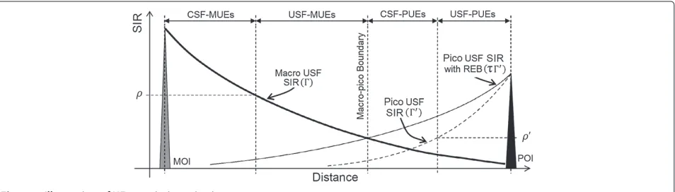
The cell selection process using, , and the REB τ can be explained with reference to Figure 2. Ifτis less than, then the UE is associated with the MOI, otherwise with the POI. After the cell selection, the UE is scheduled either in USF or in CSF based on the scheduling thresh-oldsρ(for MUE) andρ(for PUE). In a macrocell, ifis less thanρthen the UE is scheduled to USF, otherwise to CSF. Similarly, in a picocell, if is greater thanρ then the UE is scheduled to USF, otherwise to CSF (to pro-tect it from macrocell interference). The cell selection and

Table 1 Notations and symbols

Symbol Description

λ,λ,λu Intensities of the MBS, PBS, and UE nodes,

respectively

Ptx,Ptx Maximum transmit powers of MBS and PBS,

respectively

K,K Signal attenuation factors that account for geometrical parameters such as the transmitter/receiver antenna heights of the MBS and the PBS, respectively

P,P Effective maximum transmit powers of MBS and PBS, respectively, after considering the attenuation factorsKandK

α Power reduction factor for MBS during the transmission of CSFs

β Duty cycle for the transmission of USFs

τ Range expansion bias for picocells

ρ,_ρ Scheduling thresholds for MUEs and PUEs, respectively

r,r Distances of a UE from its MOI and POI, respectively

δ Path-loss exponent

S(r),S(r) RSRPs from the MOI and the POI, respectively

H,H Exponentially distributed random variables that account for Rayleigh fading for the transmissions from MBS and PBS, respectively

Z,Z Total interference power at a UE during USF and CSF, respectively

γ,_γ SIRs from MOI and POI, respectively, during USFs

γcsf,γcsf SIRs from MOI and POI, respectively, during

CSFs

N_usf,N_usf,N_csf,N_csf Mean number of USF-MUEs, USF-PUEs, CSF-MUEs, and CSF-PUEs, respectively, in a cell

Cusf,Cusf,Ccsf,Ccsf Mean aggregate SEs for USF-MUEs, USF-PUEs,

CSF-MUEs, and CSF-PUEs, respectively, in a cell

Cu,usf,C_u,usf ,Cu,csf,C_u,csf Per-user SEs for USF-MUEs, USF-PUEs,

CSF-MUEs, and CSF-PUEs, respectively, in a cell

Csum,Clog Sum of capacities and sum of log capacities in

a cell

scheduling conditions can be combined and formulated as follows:

If > τand≤ρ→USF-MUE, (6)

If > τ and > ρ→CSF-MUE, (7) If≤τ and> ρ→USF-PUE, (8)

If≤τ and≤ρ→CSF-PUE. (9)

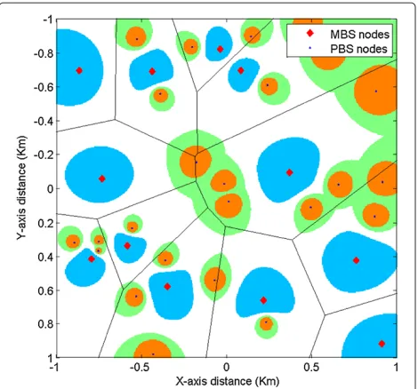
A sample layout of MBSs and PBSs with their cover-age areas for the four different UE categories is illustrated in Figure 3. Note that in the related work of [16], the UE association criteria are based on the average refer-ence symbol received power at UE, where as our model is based on the SIR at UE, it also encompasses the FeICIC mechanism. In [16], the boundary between the USF-PUEs (picocell area) and the CSF-PUEs (range expanded area) is fixed due to the fixed transmit power of PBS. On the other hand, in our approach, the boundary between USF and CSF users can be controlled using ρ in the macro-cell andρ in the picocell, the parameters which play an important role during optimization as will be shown in Section 5.3.

Using (1) to (5), it can be shown that the two SIRscsf and_csfcould be expressed in terms ofandas

csf=α,csf =

₍₁₊₎

1+[α (+1)−]. (10) Hence, knowing the statistics of and, particularly theirjoint probability density function(JPDF), would pro-vide a complete picture of the SIR statistics of the HetNet system. We first derive an expression for joint comple-mentary cumulative distribution function (JCCDF) of and in Section 3.1. Then, we differentiate the JCCDF with respect toγ andγto get the expression for JPDF in Section 3.2, which will then be used for spectral efficiency analysis.

Figure 3Illustration of two-tier HetNet layout.In picocells, the coverage regions for USF- and CSF-PUEs are colored in orange and green, respectively, whereas in macrocells, the coverage regions for USF- and CSF-MUEs are colored in white and blue, respectively.

3 Derivation of joint SIR distribution 3.1 JCCDF ofand

From (1), we know thatS(r)andS(r)are exponentially distributed with meanP/rδandP/(r)δ, respectively. For brevity, substituteS(r)=XandS(r)=Yin (2) and (3):

= X

Y+Z, ₌ Y

X+Z. (11)

Using (11), it can be easily shown that the product has a maximum value of 1.

Let,RandRbe the random variables denoting the dis-tances of MOI and POI from a UE. Then, the JCCDF of andconditioned onR=r,R=ris given by

P > γ,> γR=r,R=r

=EZ

PX> γ (Y+Z),Y > γ(X+Z),

=EZ

+∞

y1

fY(y)

y/γ_−Z

γ (y+Z) fX(x)dxdy

,

(12)

for γ > 0, γ > 0, and γ γ < 1. Here, fX(x) = r δ

P

exp −r_Pδx, fY(y) = (r

₎δ

P exp

−(r)δ

P y

, and the

inte-gration limity1 = γZ

1+γ 1−γ γ

. The integration region of (12) is graphically represented in Figure 4. By solving

Figure 4Illustration of the integration region in the JPDF ofX

andY.The shaded region indicates the integration region in order to compute the JCCDF.

the integration as shown in Appendix 1, we can obtain a closed form expression for the conditional JCCDF as

P > γ,> γ|R=r,R=r

= (1−γ γ

_)L

Z

1 1−γ γ

γ (1+γ_)rδ

P +

γ_{(1+γ )(r)}δ

P

1+γP_Prr δ

1+γ_PP

r r

δ ,

(13)

forγ >0,γ>0, andγ γ<1, whereLZ(s)is the Laplace

transform of the total interferenceZ.

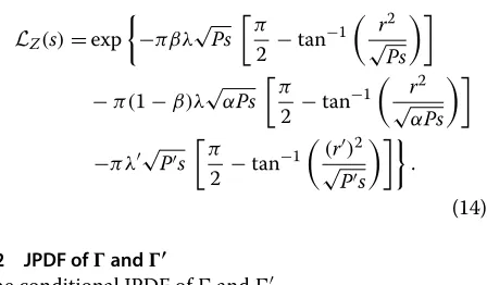
Expression for LZ(s) can be derived as follows. We assume that the interfering MBSs of a UE are frame asynchronous and subframe synchronous. Essentially, we wanted to assume no synchronization at all. However, this would permit part of a subframe from an interfering trans-mitter to interfere with part of another subframe at the receiver, and the complications for analysis would be too much. To simplify the interference scenario, we would not account for, or model, any interference by partially over-lapping subframes. In other words, if a subframe partially overlaps another subframe, it is assumed to overlap com-pletely. This is equivalent to the ‘subframe-synchronized but frame-asynchronous’ assumption.

be modeled using three independent PPPs as illustrated in Table 2.

Let Iusf(r), Icsf(r), andI(r) be the interference at UE from all interfering USF-MBSs, CSF-MBSs, and PBSs. Then, the total interference is Z = Iusf(r) + Icsf(r) +

I(r). Using ([26], Corollary 1), parameters in Table 2, and assumingδ=4, we can derive the Laplace transform ofZ

in (13) to be

can be derived by differentiating the JCCDF in (13) with respect to γ and γ. Detailed derivation of conditional probability JPDF is provided in Appendix 2. Using the theorem of conditional probability, we can write

f,_,R,Rγ,γ,r,r=f,_|R,R γ,γr,rfR(r)fR

, respectively. We can then express the unconditional JPDF ofandas

f,γ,γ= satisfies the minimum distance constraints: UE should be located at distances of at leastdminfrom the MOI anddmin from the POI.

Table 2 PPP parameters for USF MBSs, CSF MBSs, and PBSs

BS type PPP Intensity Tx. power Distance of UE to nearest BS

USF-MBSs _{usf βλ} P r

CSF-MBSs _{csf (}1_{−β)λ α}P r

PBSs _λ P r

4 Spectral efficiency analysis

In this section, the expressions for aggregate and per-user SEs for different UE categories are derived. Considering the JPDF of an arbitrary UE in (17), first, the expressions for the probabilities that the UE belongs to each category are derived. Then, these expressions are used to derive the mean number of UEs of each category in a cell. These are followed by the derivation of the aggregate SE. Then, per-user SE expressions are obtained by dividing the aggregate SE by the mean number of UEs.

4.1 MUE and PUE probabilities

Depending on the SIRs and , a UE can be one of the four types: USF-MUE, MUE, USF-PUE, or CSF-PUE. Given that the UE is located at a distancerfrom its MOI andrfrom its POI, probabilities of the UE belonging to each type can be found by integrating the conditional JPDF over the regions whose boundaries are set by the cell selection conditions in (6) to (9). Based on these condi-tions, the integration regions for different UE categories are shown in Figure 5.

The probability that a UE is a CSF-MUE can be found by integrating the JPDF over the region R1,

Pcsf=P

To form concise equations, let us define an integral function

wheregis a function ofγ andγ, and Rifori = 1, 2, 3, 4 is the integration region as defined in Figure 5. Then, (18) can be written as

Pcsf=P

> τ, > ρ=G(1, R1). (20) Similarly, the conditional probabilities that a UE is a USF-MUE, USF-PUE, or CSF-PUE are respectively given as 4.2 Mean number of MUEs and PUEs

Since the MBS locations are generated using PPPs, the coverage areas of all the MBSs resemble a Voronoi tessel-lation. Consider an arbitrary Voronoi cell. Let the number of UEs in the cell beNand the number of CSF-MUEs in the cell beM. Then,Mis a random variable, and the mean number of CSF-MUEs is given by

Ncsf=E[M]=E

where in (24) we use the fact that the probability that any of theN UEs in a cell being a CSF-MUE is independent ofN. However, it is important to note that this is itself a consequence of our assumption that there is no limit on the number of CSF-MUEs per cell. Further, the event that any of the UEs in a cell is a CSF-MUE is independent of the event that any other UE in that cell is a CSF-MUE, and all such events have the same probability of occurrence, namelyPcsfgiven in (20). Then,

Ncsf=EN

Using ([27], Lemma 1), it can be shown that the mean number of UEs in a Voronoi cell isλu/λ. Therefore, the mean number of CSF-MUEs in a cell is given by

Ncsf=

Pcsfλu

λ . (26)

Similarly, the mean number of USF-MUEs, USF-PUEs, and CSF-PUEs is respectively given by

Nusf=

4.3 Aggregate and per-user spectral efficiencies

We use Shannon capacity formula, log₂(1+SIR), to find the SE of each UE type. The mean aggregate SE of an arbitrarily located CSF-MUE can be found by

Ccsfλ,λ,τ,α,ρ,β=(1−β)E

Similarly, the mean aggregate SEs for MUEs, USF-PUEs, and CSF-PUEs can be respectively derived to be

Cusf

4.4 5th percentile throughput

The 5th percentile throughput reflects the throughput of cell-edge UEs. Typically, the cell-edge UEs experience high interference, and analyzing their throughput pro-vides important information about the fairness among the users in a cell and the system performance.

Consider the JPDF expression in (17). The integration regions of the JPDF for different UE categories are shown in Figure 5. The SIR PDF of USF-MUEs can be evaluated by integrating the JPDF overγin region R2,

for 0≤γ ≤ρ. The CDF expression can be derived as

F(γusf)=P{≤γusf|UE is a USF-MUE} = γusf

0

f(γ )dγ= γusf

0

min

γ τ,1γ

0

f,

γ,γdγdγ,

(37)

for 0≤γusf≤ρ, and the CDF of throughput of the USF-MUEs can be derived as a function ofF(γusf)in (37) as

FCusf(cusf)=P{Cusf≤cusf|UE is a USF-MUE}

=Plog₂(1+usf)≤cusf|UE is a USF-MUE

, =Pusf≤(2cusf−1)|UE is a USF-MUE

=F(2cusf−₁)_,

(38)

for 0≤cusf≤log2(1+ρ). By using the CDF plots, the 5th percentile throughput of USF-MUEs can easily be found as the value at which the CDF is equal to 0.05. Similarly, the 5th percentile throughput of other three UE categories can also be found.

5 Numerical and simulation results

The average SE and 5th percentile throughput expressions derived in the earlier sections are validated using a Monte Carlo simulation model built in MATLAB. Validation of the PPP capacity results for a HetNet scenario with range expansion and reduced power subframes is a non-trivial task. In this section, details of the simulation approach used for validating the PPP analyses are explicitly doc-umented to enable reproducibility. MATLAB codes for the simulation model, and the theoretical analysis can be downloaded from [24].

5.1 Simulation methodology for verifying PPP model The algorithm used in the simulation to find the aggregate and per-user SEs is described below.

1. TheX- andY-coordinates of MBSs, PBSs, and UEs are generated using uniformly distributed random variables. The mean number of MBS and PBS location marks isλAandλA, respectively, whereA is the assumed geographical area that is square in shape as illustrated in Figure 6.

2. In the PPP analysis, the geographical area is assumed to be infinite. In such case, it is important to account foredge effects in the simulations. In a tessellation that is defined on an unbounded region, what happens outside a bounded simulation window may effect what happens within the window [28]. As the simulation area is limited, if a UE is located at the edge of the simulation area, the BSs around it will not be symmetrically distributed. Hence, to avoid the edge effects, the UE locations are constrained within

−6 −4 −2 0 2 4 6

−6 −4 −2 0 2 4 6

Y−axis distance (Km)

X−axis distance (Km)

UEs PBSs MBSs

Area A

Area A_u

Figure 6Simulation layout.

a smaller areaAuthat is aligned at the center of the main simulation areaAto avoid the UEs from being located at the edges. The mean number of UEs in the areaAuisλuAu.

3. The MOI (closest MBS) and POI (closest PBS) for each UE are identified. The minimum distance constraints are applied by discarding the UEs that are closer thandmin(dmin )from their respective MOIs (POIs).

4. The SIRs,,csf, andcsfare calculated for each UE using (2) to (5).

5. The UEs are classified as USF-MUEs, CSF-MUEs, USF-PUEs, and CSF-PUEs using the conditions in (6) to (9).

6. The MUEs (PUEs) which share the same MOI (POI) are grouped together to form the macro- and picocells.

7. The SEs of all the UEs are calculated. In a cell, SE of a USF-MUEiis calculated using βlog2(1+i)

(No. of USF-MUEs in the cell). The SEs of other UE types are calculated using similar formulations.

8. The aggregate capacity of each UE type is calculated in all the cells.

9. Mean aggregate capacity and mean number of UEs of each type are calculated by averaging over all the cells. 10. The per-user SE of each UE type is calculated by

(mean aggregate capacity)/(mean number of UEs).

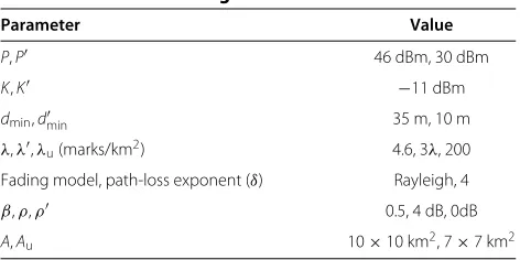
Table 3 Parameter settings

Parameter Value

P,P 46 dBm, 30 dBm

K,K ₋11 dBm

dmin,dmin 35 m, 10 m

λ,_λ,_λu(marks/km2) 4.6, 3λ, 200

Fading model, path-loss exponent (δ) Rayleigh, 4

β,ρ,ρ 0.5, 4 dB, 0dB

A,Au 10×10 km2, 7×7 km2

to Figure 6, the inner simulation areaAuwhere the UEs are distributed consists of a random number of macrocells and picocells in each simulation instance. On average, it containsλAumacrocells andλAupicocells. Since the sim-ulation results are obtained by averaging over the macro-cells and picomacro-cells, we can say that the simulation results were obtained by averaging over approximatelyλAuNsim macrocells andλAuNsimpicocells, whereNsimis the num-ber of simulation instances. Using the parameter values in Table 3 andNsim = 20, we can say that the simulation results were obtained by averaging over approximately 4,508 macrocells and 13,524 picocells.

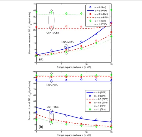
The analytic and simulation plots in Figure 7a,b match with sufficient accuracy. However, there exists a slight dis-agreement between the analytic and simulation results which could be due to the fact that the calculation of analytic results involves four nested integrals. Since the numerical integration in MATLAB has certain tolerance limits, the results could be off the ideal values. Another source for disagreement could be due to the fact that in theoretical analysis, the BSs are assumed to be distributed over an infinite geographical area. However, the simula-tions are performed using a finite area of 10×10 km2. Nevertheless, Figure 7 provides the following insights.

5.2.1 USF- and CSF-MUEs

Referring to Figure 2, USF-MUEs form the outer part and CSF-MUEs form the inner part of the macrocell. As the REB increases, some of the USF-MUEs at the macro-pico boundary which have worse SIRs are offloaded to the picocell. Consequently, the mean number of USF-MUEs decreases and their per-user SE increases as shown in Figure 7a.

The mean number of CSF-MUEs are not affected byτ as long as√τ ≤ ρ. Considering Figure 5, it can be noted that if√τ = ρ, the lineγ = τγ intersects the bound-ary of region R1. Hence, ifτis increased further such that √_{τ > ρ}

, the area of R1 decreases and thereby decreases the mean number of CSF-MUEs. Therefore, the per-user SE of CSF MUEs remains constant as long as√τ ≤ρand increases ifτ crosses this limit as shown in Figure 7a.

On the other hand, as the α increases, the trans-mit power of all the interfering MBSs increases dur-ing CSFs; hence, it increases the interference power

Z at all the UEs. This causes the SIRs of USF-MUEs (), USF-PUEs (), and CSF-PUEs (_csf) to decrease, which can be noted in (2), (3), and (5), respectively. However, the SIRs of CSF-MUEs (csf) would increase (despite of increased interference) because of the increase in received signal power (due to higher α) which can be noted in (4). Considering (6) and (7), since ρ is a constant, the degradation in causes the number of USF-MUEs to increase and CSF-MUEs to decrease. Con-sequently, the per-user SE of USF-MUEs decreases and that of CSF-MUEs increases for increasingα, as shown in Figure 7a.

5.2.2 USF- and CSF-PUEs

As the REB increases, the mean number of USF-PUEs remains constant if ρ > 1/√τ because the area of region R4 in Figure 5 is unaffected by the value of τ. Therefore, the per-user SE of USF-PUEs also remains constant for increasing REB as shown in Figure 7b. With increasing REB, some MUEs are offloaded to the picocell and become CSF-PUEs. But these UEs are located at cell-edges and have low SIRs. Hence, the per-user SE of CSF-PUEs decreases as shown in Figure 7b.

On the other hand, as the α increases, the transmit power of all the interfering MBSs increases during CSFs causing, , and _csf to decrease andcsfto increase, as explained previously. Considering (8) and (9), sinceρ is a constant, the degradation incauses the number of USF-PUEs to decrease and CSF-PUEs to increase. Con-sequently, the per-user SE of USF-PUEs increases and that of CSF-PUEs decreases for increasingα, as shown in Figure 7b.

5.3 Optimization of system parameters to achieve maximum capacity and proportional fairness

The five parametersτ, α, β, ρ, andρare the key system parameters that are critical to the satisfactory perfor-mance of the HetNet system. The goal of these param-eter settings is to maximize the aggregate capacity in a cell while providing proportional fairness among the users.

Consider an arbitrary cell which consists ofNUEs. Let

Cibe the capacity of an arbitrary UEi∈ {1, 2,. . ., N}. The

sum of capacities (sum-rate) and the sum of log capacities (log-rate) in a cell are respectively given by

Csum=

N

i=1

Ci, Clog=

N

i=1

log(Ci)=log

_N

i=1

Ci

.

0 5 10 15 0

5 10 15 20 25 30 35 40 45

Range expansion bias,τ (in dB)

Per−user macrocell SE x

λ u

(bps/hertz)

α = 0 (Sim)

α = 0 (PPP)

α = 0.5 (Sim)

α = 0.5 (PPP)

α = 1 (Sim)

α = 1 (PPP)

0 5 10 15

0 10 20 30 40 50 60 70 80 90 100

Range expansion bias,τ (in dB)

Per−user picocell SE x

λ u

(bps/hertz) α = 0 (PPP)

α = 0 (Sim)

α = 0.5 (PPP)

α = 0.5 (Sim)

α = 1 (PPP)

α = 1 (Sim) CSF−MUEs

USF−MUEs

(a)

USF−PUEs

(b)

CSF−PUEs

Figure 7Per-user SE in (a) macrocell and (b) picocell.For the case withβ= 0.5,ρ= 4 dB, andρ= 0 dB.

Maximizing the Csum corresponds to maximizing the aggregate capacity in a cell, while maximizing the Clog corresponds to proportional fair resource allocation to the users of a cell ([29], App. A) [30]. There can be trade-offs existing between aggregate capacity and fair-ness in a cell. Maximizing theCsummay reduce theClog and vice versa. In this section, we try to understand these trade-offs by analyzing the characteristics of Clog and Csum with respect to the variation of key system parameters.

We attempt to maximize the aggregate capacity and the proportional fairness among the users by jointly

optimizing the five key system parameters which can be mathematically formulated as

max

ρ,ρ_,α,τ,βCsum=_ρ,ρmax_,α,τ,β

N

i=1

Ci, (40)

and

max

ρ,ρ_,α,τ,β Clog=_ρ,ρmax_,α,τ,β log

_N

i=1

Ci

. (41)

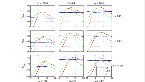
for an optimum solution in a five-dimensional space. The variation ofClogwith respect toρ, ρ, α, andτ is shown in Figure 8, forβ =0.5. These plots are obtained through the Monte Carlo simulations, and each plot is the varia-tion ofClogwith respect toρfor fixed values ofρ,α, and τ. The optimum scheduling thresholdsρ∗ andρ∗ that maximize theClogare dependent on the values ofαandτ. In this paper, we have used a simple brute-force search technique to optimize the system parameters, while it is also possible to use non-linear optimization techniques. For example, reinforcement learning method is used in [31,32] to optimize the downlink transmission strategies in HetNets such as the transmit power and the REB. In [33], a game theoretic approach and distributed learn-ing algorithm are used to optimize the downlink trans-mit power, REB, and the ON/OFF states of individual BSs to minimize the system cost which includes energy and load expenditures. Typically, these optimization tech-niques use distributed approach and are developed to be efficient from the implementation perspective. In addi-tion, some information exchange among the BSs is typ-ically required for these optimization methods to work. For example, in [33], estimated traffic load, transmission power, and REB are broadcasted by the BSs for optimiza-tion of the operating parameters at each individual small cell BS. On the other hand, the brute-force search tech-nique does not require any information exchange among

the BSs. In this paper, our focus is to understand the char-acteristics of the optimum system parameters, rather than the implementation efficiency of the optimization method used. Brute-force search method is also used, for exam-ple, in [16] to find the optimum REB and duty cycle of almost blank subframes that maximize the rate coverage in HetNets.

Figure 9 shows the plots ofρ∗andρ∗as the functions of αandτ. The markers show the simulation results, while the dotted lines show the smoother estimation obtained using the curve fitting tool in MATLAB. For small α values, the optimum threshold ρ∗ has higher values as shown in Figure 9a, and according to (7), this causes very few MUEs that have > ρ∗ to be scheduled during CSFs. This makes sense because MBS transmit power during CSFs is very low for smallα, and hence, the num-ber of CSF-MUEs which can be covered is also less. On the other hand, for higherαvalues, MBS transmits with higher power level during CSFs and can cover a larger number of CSF-MUEs. Therefore, to improve the fair-ness proportionally, the optimalρ∗value decreases with increasing α so that more MUEs are scheduled during CSFs.

In the picocell, with increasing α, the CSF-PUEs at the cell edges will experience higher interference from the MBSs. Then, more PUEs should be scheduled dur-ing USFs to improve proportional fairness. Likewise,

−110 −105 −100 −95 −90

C log

ρ′ = −10 dB ρ′ = 4 dB ρ′ = 20 dB

−95 −90 −85 −80 −75

−10 0 10 20

−80 −75 −70 −65

ρ (in dB)

−10 0 10 20

ρ (in dB)

−10 0 10 20

ρ (in dB) α=0

α=0.5

α=1

τ = 6 dB

τ = 0 dB

τ = 12 dB C log

C log

0 0.2 0.4 0.6 0.8 1 0

5 10 15 20

0 0.2 0.4 0.6 0.8 1

−5 0 5 10 15

Power reduction factor, α

τ = 0 dB τ = 6 dB τ = 12 dB

τ = 0 dB τ = 6 dB τ = 12 dB (a)

(b)

ρ

* (dB)

ρ′

* (dB)

Figure 9Optimized scheduling thresholds versusαfor different

τ(a) in macrocell and (b) in picocell.Withλ=4.6 marks/km2and λ_{=13.8 marks/km}2_.

decreasingρ∗in Figure 9b indicates that more PUEs are scheduled during USFs as per (8).

The Clog with optimum scheduling thresholdsρ∗ and ρ∗_{is plotted in Figure 10. The higher theC}

log, the better is the proportional fairness. It is important to note that the range expansion bias,τ, has a significant effect on propor-tional fairness. TheClogincreases from−40 to−28 when τ is increased from 0 to 12 dB.

Compared toτ, α has a smaller effect on the propor-tional fairness. Whenαis set to zero which corresponds to the eICIC,Clogis at its minimum. It shows that eICIC pro-vides minimum proportional fairness. Figure 10 moreover shows that setting α = 1, which corresponds to no eICIC, also does not provide maximumClog. Anαsetting

0 0.2 0.4 0.6 0.8 1

−100 −95 −90 −85 −80 −75 −70 −65 −60

Power reduction factor, α C log

τ = 0 dB τ = 6 dB τ = 12 dB

Ideal range for proportional fairness

Figure 10Clogversusαwith optimum scheduling thresholdsρ∗

and_ρ∗.With_λ=4.6 marks/km2_{andλ=13.8 marks/km}2_.

between 0.125 and 0.5 maximizes theClogand hence the proportional fairness.

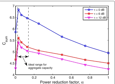
The characteristics of Csum with optimum scheduling thresholds are shown in Figure 11. As the τ increases,

Csum decreases, which is the opposite effect when com-pared to the Clog in Figure 10. This shows the trade-off between the aggregate capacity and the proportional fair-ness. Increasing the τ would increase the proportional fairness but decrease the aggregate capacity, and vice versa.

Comparing Figures 10 and 11 also explains the trade-off associated with setting α. A very small value, 0 < α < 0.125, provides largerCsumbut smallerClog, which is better from an aggregate capacity point of view. Set-ting 0.125 ≤ α ≤ 0.5 is better from a fairness point of view. Any value of α > 0.5 is not recommended since it degrades the aggregate capacity as shown in Figure 11, decreases the proportional fairness as shown in Figure 10, and consumes higher transmit power by the MBSs. Set-tingα = 0 as in the eICIC case would reduce bothCsum andClogdrastically.

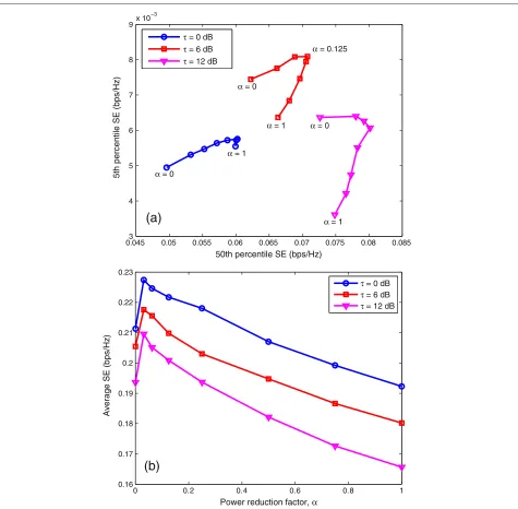
The effects ofα andτ on the 5th percentile, 50th per-centile, and average SEs are shown in Figure 12. Here again, optimum scheduling thresholds ρ∗ and ρ∗ are used. Figure 12a shows that as the REB increases from 0 to 6 dB, some of the MUEs at the border of the macrocell are offloaded to the picocell. Since these offloaded UEs are served by picocell during the CSFs, they would have better throughput, resulting in the improvement in the 5th per-centile SE. However, if the REB increases to 12 dB, more MUEs are offloaded and the picocell becomes crowded resulting in poor SEs for the PUEs. Hence, the 5th per-centile SE decreases when the REB increases from 6 to 12 dB. Figure 12a also shows that withτ = 6 dB, setting α = 0.125 maximizes both the 5th and 50th percentile

0 0.2 0.4 0.6 0.8 1

4 4.5 5 5.5 6 6.5 7

Power reduction factor, α C sum

τ = 0 dB τ = 6 dB τ = 12 dB

ideal range for aggregate capacity

Figure 11Csumversusαwith optimum scheduling thresholdsρ∗

0.0453 0.05 0.055 0.06 0.065 0.07 0.075 0.08 0.085 4

5 6 7 8 9x 10

−3

50th percentile SE (bps/Hz)

5th percentile SE (bps/Hz)

τ = 0 dB

τ = 6 dB

τ = 12 dB

0 0.2 0.4 0.6 0.8 1

0.16 0.17 0.18 0.19 0.2 0.21 0.22 0.23

Power reduction factor, _α

Average SE (bps/Hz)

τ = 0 dB

τ = 6 dB

τ = 12 dB

α = 0.125

α = 0

α = 1

α = 1

α = 0

α = 0

α = 1

(b)

(a)

Figure 12Effects ofαandτon the 5th percentile, 50th percentile, and average SEs.(a)5th percentile SE versus 50th percentile SE.(b) Average SE versus power reduction factorα. Withλ=4.6 marks/km2_{andλ=13.8 marks/km}2_.

SEs. Figure 12b shows the characteristics of average SE of an arbitrary UE, which is similar to the characteristics ofCsum in Figure 11. By comparing Figure 12a,b, it can be noted that the 50th percentile SE and the average SE have opposite behaviors with respect to the REB. As the REB increases, the 50th percentile SE increases while the average SE decreases.

5.4 Impact of the duty cycle of uncoordinated subframes In the results of Figures 9, 10, 11, and 12,β was set to 0.5 and we next show the effect of varyingβ onClogand

Csum. Introducingβinto the optimization problem makes it difficult to visualize the results due to the addition of one more dimension. Therefore, we use the optimized scheduling thresholds,ρ∗ andρ∗, and analyzeClog and

Csumas the functionsβ,α, andτ. Figures 13 and 14 show theClogversusβ and theCsumversusβ, respectively, for different values of α and τ. The variation of Clog with respect toβ is not significant, except forα = 0, whereas the variation ofCsumwith respect toβis significant.

0.1 0.2 0.3 0.4 0.5 0.6 0.7 0.8 0.9 −115

−110 −105 −100 −95 −90 −85 −80 −75 −70 −65 −60

USF duty cycle, β Clog

α = 0 α = 0.25 α = 0.5 α = 1 τ = 12 dB

τ = 6 dB

τ = 0 dB

Figure 13Clogversusβwith optimum scheduling thresholdsρ∗

andρ∗.Withλ=4.6 marks/km2andλ=13.8 marks/km2.

performance in the previous paragraphs, and hence, it is not recommended. For other values ofα, variation in β does not affect the Clog significantly, which shows that by using a fixed value ofβ, proportional fairness can be achieved by optimizing (to maximizeClog) the scheduling thresholds. Figure 14 shows that fixingβapproximately to 0.43 maximizes theCsumirrespective ofαandτ, provided the scheduling thresholds are optimized to maximizeClog. In [16], the boundary of CSF-PUEs that form the inner region of picocell (excluding the range expansion region) is fixed due to the fixed transmit power of PBS. The asso-ciation biasandresource partitioning fractionparameters are used as the variables to be optimized. It is analogous for us to have a fixedρand optimizeβandτ. But in con-trast, we fix the β for simplicity and optimize the other four parameters, since coordinating β among the cells through the X2 interface is complex and adds to com-munication overhead in the backhaul. The X2 is a type of interface in LTE networks which connects neighboring eNodeBs in a peer-to-peer fashion to assist handover and provide a means for rapid coordination of radio resources [34].

5.5 5th percentile throughput

Using the expressions derived in Section 4.4, the 5th per-centile throughput versus α for differentτ is shown in Figure 15a for MUEs and in Figure 15b for PUEs. As the α increases, MBSs transmit at a higher power level dur-ing CSFs, and the UEs of all types experience a higher interference power. However, the received signal power at CSF-MUEs increases withα and results in improved 5th percentile throughput as shown in Figure 15a. But the SIRs of USF-MUEs and USF/CSF-PUEs degrade due to higher interference, and therefore, their 5th percentile throughput decreases with increase in α as shown in Figure 15a,b.

0 0.2 0.4 0.6 0.8 1

0 1 2 3 4 5 6 7 8

τ = 0 dB

C sum

(bps/Hz)

USF duty cycle, β

α = 0

α = 0.25

α = 0.5

α = 1

0 0.2 0.4 0.6 0.8 1

0 1 2 3 4 5 6 7 8

C sum

(bps/Hz)

USF duty cycle, β

τ = 6 dB

α = 0

α = 0.25

α = 0.5

α = 1

0 0.2 0.4 0.6 0.8 1

0 1 2 3 4 5 6 7 8

C sum

(bps/Hz)

USF duty cycle, β

τ = 12 dB

α = 0

α = 0.25

α = 0.5

α = 1

β* = 0.43

β* = 0.43

β* = 0.43

Figure 14Csumversusβwith optimum scheduling thresholdsρ∗

andρ∗.Withλ=4.6 marks/km2_{andλ=13.8 marks/km}2_.

0 0.2 0.4 0.6 0.8 1 0

0.5 1 1.5 2 2.5

Power reduction factor, α

5th percentile throughput (bps/Hz)

0 0.2 0.4 0.6 0.8 1

0 0.5 1 1.5 2 2.5 3 3.5 4 4.5 5

Power reduction factor, _α

5th percentile throughput (bps/Hz)

τ = 0 dB (Sim)

τ = 0 dB (PPP)

τ = 6 dB (Sim)

τ = 6 dB (PPP)

τ = 12 dB (Sim)

τ = 12 dB (PPP)

CSF−PUEs USF−PUEs

(a)

(b)

USF−MUEs CSF−MUEs

Figure 155th percentile throughput (a) in macrocell and (b) in picocell.Withλ=4.6 marks/km2_{andλ=13.8 marks/km}2_.

offloaded UEs in the picocell are scheduled during CSFs, and due to their poor SIR, the 5th percentile throughput of CSF-PUEs decreases as shown in Figure 15b.

5.6 Comparison with real BS deployment

We obtained the data of real BS locations in United King-dom from an organization [25] where the mobile network operators have voluntarily provided the information of location and operating characteristics of individual BSs. The data set in [25] was last updated in May 2012, and it provides exact locations of the BSs. Also, the BSs of different operators can be distinguished.

−0.2 −0.15 −0.1 −0.05 0 51.44

51.46 51.48 51.5 51.52 51.54 51.56 51.58

Longitude (in deg.)

Real BS locations

−0.2 −0.15 −0.1 −0.05 0

51.44 51.46 51.48 51.5 51.52 51.54 51.56 51.58

Longitude (in deg.)

Operator−2, MBS density = 3.81 MBSs/Km2

Real BS locations Operator−1, MBS density = 1.53 MBSs/Km2

Latitude (in deg.)

Latitude (in deg.)

Figure 16Real base station locations of two different operators in a15×15km2area of London city.

the PBS densityλ was varied to analyze its effect on the 5th percentile SE.

The plots of 5th percentile SE versus PBS density are shown in Figure 17 for the two operators. The 5th per-centile SE of operator-2 is better than that of operator-1 since the former has higher MBS density. As expected, the 5th percentile SE improves with the increase in PBS density. It can also be observed that increasing the PBS transmit powerPfrom 10 to 30 dBm will result in almost twice the 5th percentile SE. Since the hexagonal grid model is an ideal case, it has the best 5th percentile SE and forms an upper bound. The PPP model has a worse 5th percentile SE and forms a lower bound. The real MBS deployment is usually planned, and hence, it is not com-pletely random in nature. On the other hand, it is also not equivalent to the idealized hexagonal grid model due to

0 5 10 15 20

0 0.005 0.01 0.015 0.02

PBS density to MBS density ratio, λ′/λ Hex−grid

Real MBS Random (PPP)

0 5 10 15 20

0 0.005 0.01 0.015 0.02 0.025 0.03 0.035

PBS density to MBS density ratio, λ′/λ Hex−grid

Real MBS Random (PPP)

Operator−1, MBS density = 1.53 MBSs/Km2

P′ = 30 dBm

P′ = 10 dBm

Operator−2, MBS density = 3.81 MBSs/Km2

P′ = 10 dBm P′ = 30 dBm

5th percentile SE (bps/hertz)

5th percentile SE (bps/hertz)

Figure 175th percentile SE versus PBS density.

the practical constraints involved during the deployment. Hence, the 5th percentile SE of real MBS deployment lies in between the two bounds of hexagonal grid and random deployments.

6 Conclusions

HetNet with reduced power subframes yields better per-formance than that with almost blank subframes (eICIC) in terms of both aggregate capacity and proportional fair-ness. However, transmitting the reduced power subframes with greater than half the maximum power proved to be inefficient because it degrades both the aggregate capacity and the proportional fairness. Increasing the range expan-sion bias improves the proportional fairness but degrades the aggregate capacity. In the case of eICIC, the duty cycle of almost blank subframes has a significant effect on the fairness, but with reduced power subframes and optimized scheduling thresholds, duty cycle has a lim-ited effect on fairness. Hence, fixing the duty cycle and optimizing the scheduling thresholds is preferable since it avoids the overhead of coordinating the duty cycle among the cells through the X2 interface. We also compared the 5th percentile SE results from the PPP model with those from the real BS deployment and hexagonal grid model. We observed that the hex grid model forms the upper bound while the PPP model forms the lower bound. Increasing the PBS density or the PBS transmit power would improve the 5th percentile SE.

In this paper, we considered SIR as the only deciding fac-tor for UE association. However in real LTE networks, UE association criteria also include factors such as UE veloc-ity, load conditions in cells, and backhaul capacity. Our future work includes taking such factors into account for capturing a wider range of deployment scenarios.

Appendix 1

Derivation of JCCDF expression

This part of the appendix derives closed form equation for the JCCDF in (12). Let us start by rewriting the JCCDF expression

The inner integral in (42) can be derived as

y/γ_−Z

Then, the outer integral in (42) can be derived as

+∞

The first term in right-hand side (RHS) of (46) can be evaluated as

The second term in RHS of (46) can be evaluated as

λy

By substituting (47) and (48) in the first and second terms of (46) respectively, we get

_+∞

Substituting (49) in (42) and using (44), we get

P > γ,> γ|R=r,R=r

Using the definition of Laplace transform, EZ

Appendix 2

Derivation of JPDF expression

Assuming δ = 4, the JCCDF expression in (51) can be rewritten as

After some tedious but straightforward algebraic steps, it can be shown that

M1=

We can derive the JPDF by differentiating the JCCDF (52) with respect toγ andγ,

whereM1andM2are given by (55) and (56), respectively. By solving (59), it can be shown that the conditional JPDF

f,_|R,Rγ,γr,r=M2h

BS: Base station; CSF: Coordinated subframe; eICIC: Enhanced inter-cell interference coordination; FeICIC: Further enhanced inter-cell interference coordination; HetNet: Heterogeneous network; MBS: Macro base station; MOI: Macrocell of interest; MUE: Macro user equipment; PBS: Pico base station; PPP: Poisson point process; POI: Picocell of interest; PUE: Pico user equipment; REB: Range expansion bias; SE: Spectral efficiency; UE: User equipment; USF: Uncoordinated subframe.

Competing interests

The authors declare that they have no competing interests.

Acknowledgements

This research was supported in part by the U.S. National Science Foundation under the Grant CNS-1406968. Publication of this article was funded in part by Florida International University Open Access Publishing Fund.

Author details

1_{Department of Electrical and Computer Engineering, Florida International} University, 10555 W Flagler Street, Miami, FL 33174, USA.2_DOCOMO Innovations, Inc., 3240 Hillview Avenue, Palo Alto, CA 94304, USA.

Received: 26 February 2014 Accepted: 6 November 2014 Published: 12 November 2014

References

1. H Elsawy, E Hossain, M Haenggi, Stochastic geometry for modeling, analysis, and design of multi-tier and cognitive cellular wireless networks: a survey. IEEE Commun. Surv. Tutorials.15(3), 996–1019 (2013) 2. JG Andrews, F Baccelli, RK Ganti, A tractable approach to coverage and

rate in cellular networks. IEEE Trans. Commun.59(11), 3122–3134 (2011) 3. RK Ganti, F Baccelli, JG Andrews, inProceedings of the IEEE Int. Conf.

Commun. (ICC),A new way of computing rate in cellular networks, (Kyoto, Japan, 2011), pp. 1–5

4. JG Andrews, RK Ganti, M Haenggi, N Jindal, S Weber, A primer on spatial modeling and analysis in wireless networks. IEEE Commun. Mag.48(11), 156–163 (2010)

5. M Haenggi, Mean interference in hard-core wireless networks. IEEE Comm. Lett.15(8), 792–794 (2011)

6. M Haenggi, JG Andrews, F Baccelli, O Dousse, M Franceschetti, Stochastic geometry and random graphs for the analysis and design of wireless networks. IEEE J. Sel. Area Comm.27(7), 1029–1046 (2009) 7. S Mukherjee, Distribution of downlink SINR in heterogeneous cellular

networks. IEEE J. Select. Areas Commun. (JSAC), Special Issue on Femtocell Networks.30(3), 575–585 (2012)

9. TD Novlan, RK Ganti, JG Andrews, inProceedings of the IEEE Global Telecommun. Conf. (GLOBECOM),Coverage in two-tier cellular networks with fractional frequency reuse (Houston, TX, 2011), pp. 1–5

10. HS Dhillon, RK Ganti, F Baccelli, JG Andrews, Modeling and analysis of K-tier downlink heterogeneous cellular networks. IEEE J. Select. Areas Commun. (JSAC), Special Issue on Femtocell Networks.30(3), 550–560 (2012) 11. S Mukherjee, inProceedings of the IEEE Int. Conf. Commun. (ICC),Downlink

SINR distribution in a heterogeneous cellular wireless network with biased cell association, (Ottawa, Canada, 2012), pp. 6780–6786 12. H-S Jo, YJ Sang, P Xia, JG Andrews, inProceedings of the IEEE Global

Telecommun. Conf. (GLOBECOM),Outage probability for heterogeneous cellular networks with biased cell association, (Houston, TX, 2011), pp. 1–5 13. C-H Lee, C-Y Shih, Y-S Chen, Stochastic geometry based models for

modeling cellular networks in urban areas. Springer Wireless Networks. 19(6), 1063–1072 (2013)

14. OpenCellID Website. www.opencellid.org. Accessed 2 August 2013 15. D López-Pérez, Güvenç I, G de la Roche, M Kountouris, TQS Quek, J Zhang,

Enhanced inter-cell interference coordination challenges in heterogeneous networks. IEEE Wireless Commun. Mag.18(3), 22–31 (2011)

16. S Singh, JG Andrews, Joint resource partitioning and offloading in heterogeneous cellular networks. IEEE Trans. Wireless Commun.13(2), 888–901 (2014)

17. S Singh, HS Dhillon, JG Andrews, Offloading in heterogeneous networks: modeling, analysis, and design insights. IEEE Trans. Wireless Commun. 12(5), 2484–2497 (2013)

18. S Mukherjee, I Guvenc, inProceedings of the IEEE Asilomar Conf. Sig., Syst., Computers,Effects of range expansion and interference coordination on capacity and fairness in heterogeneous networks, vol. 1 (Monterey, CA, 2011), pp. 1855–1859

19. A Merwaday, S Mukherjee, I Guvenc, inProceedings of the IEEE Global Commun. Conf. (GLOBECOM),On the capacity analysis of hetnets with range expansion and eICIC, (Atlanta, GA, 2013)

20. Panasonic, Performance study on ABS with reduced macro power. Technical Report R1-113806, 3GPP TSG-RAN WG1 (2011)

21. A Morimoto, N Miki, Y Okumura, Investigation of inter-cell interference coordination applying transmission power reduction in heterogeneous networks for LTE-advanced downlink. IEICE Trans. Commun.E96-B(6), 1327–1337 (2013)

22. M Al-Rawi, J Huschke, M Sedra, inProceedings of the IEEE Int. Conf. Computer Commun. Net. (ICCCN),Dynamic protected-subframe density configuration in LTE heterogeneous networks, (Munich, Germany, 2012), pp. 1–6

23. Overview of 3GPP Release 11 V0.1.7 (2013). http://www.3gpp.org/ specifications/releases/69-release-11. Accessed 20 January 2014 24. MPACT Lab Data Management.

http://www.mpact.fiu.edu/data-management/. Accessed 23 March 2014

25. Sitefinder Website. http://www.sitefinder.ofcom.org.uk. Accessed 04 October 2014

26. S Mukherjee, inProceedings of the IEEE Int. Conf. Commun. (ICC) Workshops, UE coverage in LTE macro network with mixed CSG and open access femto overlay, (Kyoto, Japan, 2011), pp. 1–6

27. SM Yu, S-L Kim, Downlink capacity and base station density in cellular networks. Proceedings of the IEEE SpaSWiN Workshop (in Conjunction with WiOpt), 119–124 (2013)

28. J Moller, D Stoyan, Stochastic geometry and random tessellations. Research Report R-2007-28. Department of Mathematical Sciences, Aalborg University (2007)

29. P Viswanath, DNC Tse, R Laroia, Opportunistic beamforming using dumb antennas. IEEE Trans. Inf. Theory.48(6), 1277–1294 (2002)

30. MR Jeong, N Miki, inProceedings of the IEEE 23rd Int. Symp. Personal Indoor and Mobile Radio Communications (PIMRC),A comparative study on scheduling restriction schemes for LTE-Advanced networks, (Sydney, Australia, 2012), pp. 488–495

31. M Simsek, M Bennis, I Guvenc, inProc. IEEE Globecom Workshops (GC Wkshps),Enhanced intercell interference coordination in HetNets: single vs. multiflow approach, (Atlanta, GA, 2013), pp. 725–729

32. M Simsek, M Bennis, A Czylwik, inIEEE Global Communications Conference (GLOBECOM),Dynamic inter-cell interference coordination in HetNets: a reinforcement learning approach, (Anaheim, CA, 2012), pp. 5446–5450

33. S Samarakoon, M Bennis, W Saad, M Latva-aho, inProc. IEEE International Conference on Communications (ICC). Opportunistic sleep mode strategies in wireless small cell networks (Sydney, NSW, 2014), pp. 2707–2712 34. Backhauling X2. Cambridge Broadband Networks (2011). http://cbnl.

com/sites/all/files/userfiles/files/Backhauling-X2.pdf. Accessed 8 September 2014

doi:10.1186/1687-1499-2014-189

Cite this article as:Merwadayet al.:Capacity analysis of LTE-Advanced

HetNets with reduced power subframes and range expansion.EURASIP

Journal on Wireless Communications and Networking20142014:189.

Submit your manuscript to a

journal and benefi t from:

7Convenient online submission

7Rigorous peer review

7Immediate publication on acceptance

7Open access: articles freely available online

7High visibility within the fi eld

7Retaining the copyright to your article