Real-Time GPU Accelerated Multi-View Point-Based Rendering.

ABSTRACT

MARRS, ADAM CHRISTOPHER. Real-Time GPU Accelerated Multi-View Point-Based Rendering. (Under the direction of Benjamin Watson and Christopher G. Healey.)

Research in the field of computer graphics has focused on producing realistic images by accurately simulating surface materials and the behavior of light. Since achieving photorealism requires significant computational power, visual realism and interactivity are typically adver-sarial goals. Dedicated graphics co-processors (GPUs) are now synonymous with innovation in real-time rendering and have fueled further advances in the simulation of light within real-time constraints. Important rendering effects that accurately model light transport often require eval-uating costly multi-dimensional integrals. Approximating these integrals is achieved by dense spatial sampling, and is typically implemented with GPUs as multiple rasterizations of a scene from differing viewpoints. Producing multiple renders of complex geometry reveals a critical limitation in the design of the graphics processor: the throughput optimizations that make GPUs capable of processing millions of polygons in only milliseconds also prevent them from leveraging data coherence when synthesizing multiple views. Unlike its parallel processing of vertices and post-rasterization fragments, existing GPU architectures must render views seri-ally and thusparallelize view rendering poorly. The full potential of GPU accelerated rendering algorithms is not realized by the existing single view design.

© Copyright 2017 by Adam Christopher Marrs

Real-Time GPU Accelerated Multi-View Point-Based Rendering

by

Adam Christopher Marrs

A dissertation submitted to the Graduate Faculty of North Carolina State University

in partial fulfillment of the requirements for the Degree of

Doctor of Philosophy

Computer Science

Raleigh, North Carolina

2017

APPROVED BY:

Benjamin Watson

Co-chair of Advisory Committee

Christopher G. Healey Co-chair of Advisory Committee

Robert St. Amant John Whitted

DEDICATION

For John, Cortana, Gordon, Alyx, Lara, Nathan, and Elena for teaching a young man that dreams are as real as you make them.

For the 32|neVer forgeT

BIOGRAPHY

ACKNOWLEDGEMENTS

I thank my committee for their time, advice, and encouragement. Each of you played a crucial role during my time at NC State. I extend a special thanks to Ben and Christopher. Without you two this wouldn’t have been possible.

It takes a village. Thank you to my family, whose encouragement and enduring support makes everything possible: David, Beth, Ashley, Brian, Wei, and Cali.

I owe a special debt of gratitude to Mary, Winifrede, and Tad Devan whose wisdom, foresight, selfless generosity, and love for education changed my life.

TABLE OF CONTENTS

LIST OF TABLES . . . vii

LIST OF FIGURES . . . .viii

Chapter 1 Introduction . . . 1

Chapter 2 Background. . . 5

2.1 Architecture of Modern Graphics Processors . . . 6

2.2 Point-Based Rendering . . . 10

2.3 Rendering Soft Shadows in Real Time . . . 13

2.4 Rendering Reflections in Real Time . . . 19

Chapter 3 Multi-View Point-Based Rendering in Real-Time . . . 22

3.1 Motivation . . . 22

3.1.1 Limitations of Existing Methods . . . 23

3.2 A Multi-View Rendering Design . . . 26

3.2.1 Generating Points from Polygons . . . 27

3.2.2 Parallel Image Rendering . . . 28

Chapter 4 View Warped Multi-View Soft Shadows for Area Lights . . . 33

4.1 Overview . . . 34

4.2 Algorithm . . . 35

4.2.1 Buffered VWSS . . . 36

4.2.2 Unbuffered VWSS . . . 39

4.3 Results . . . 40

4.3.1 Quality vs. Performance . . . 40

4.3.2 Performance . . . 43

4.3.3 Quality . . . 48

4.4 Conclusion . . . 51

Chapter 5 View Independent Rasterization . . . 52

5.1 View Independent Transform . . . 53

5.2 Multi-View Sampling Rate . . . 54

5.2.1 Visualizing Sampling Rate . . . 56

5.2.2 Perspective Distortion . . . 58

5.3 Sampling Projected Polygons in VIR . . . 61

5.3.1 Sub-Pixel . . . 61

5.3.2 Peri-Pixel . . . 62

5.3.3 Supra-Pixel . . . 63

5.4 Optimization Strategies . . . 65

5.4.1 Point Generation . . . 65

Chapter 6 Multi-View Effects with View Independent Rasterization . . . 72

6.1 Multi-View Soft Shadows . . . 73

6.1.1 Performance . . . 74

6.1.2 Quality . . . 78

6.1.3 Limitations . . . 81

6.2 Beyond Shadows . . . 82

Chapter 7 Conclusion . . . 85

7.1 Strengths . . . 85

7.2 Limitations . . . 86

7.3 Future Work . . . 87

7.3.1 Suggestions for Future Graphics Architectures . . . 88

LIST OF TABLES

Table 4.1 GPU performance of soft shadowing algorithms on various scenes. Multi-View algorithms use 24 depth buffers @ 120 spp (and 128 depth buffers @ 640 spp in parentheses). VWSS accelerates multi-view depth buffer rendering time∼2×-13×(highlighted blue) and improves total rendering time up to 3× (highlighted red). VWSS matches PCSS performance (bold) while producing images with less total error (RMSE). Scenes with complex geometry benefit the most from VWSS. GPU times reported in milliseconds (ms). . . 45

Table 6.1 GPU performance and memory cost of VIR point generation for 128 views (and 8 views in parentheses) for geometry of varying complexity. Point storage is measured in megabytes (MB). GPU time is measured in milliseconds (ms). 74 Table 6.2 Performance results of various multi-view point rendering methods. Each

method operates on 600,000 points. Fastest times highlighted in blue. Imple-mentations in GPU Compute are faster in all cases. GPU times are measured in milliseconds (ms). . . 75 Table 6.3 GPU performance results of rendering soft shadows using View Independent

LIST OF FIGURES

Figure 2.1 A conceptual representation of modern GPU architectures [39]. Left: the common shader core. Right: the GPU Compute threading model. Thread groups are shown in orange. . . 6 Figure 2.2 A conceptual model of the GPU graphics pipeline [39]. Fixed function stages

are shown in green and programmable stages are in blue. . . 7 Figure 2.3 The results of standard rasterization and overestimating conservative

raster-ization. For each method, pixels that produce samples for the triangle are colored grey. . . 9 Figure 2.4 Point-based rendering as illustrated in [29]. Left: Naive forward mapping of

points. Right: Splatting distributes a point’s contribution across an area of nearby pixels. . . 11 Figure 2.5 Pre-production images from Media Molecule’s video game “Dreams” using a

point-based renderer [24]. Left: high sampling density where adjacent points typically lie within the same pixel create a sharp, detailed image. Right: re-duced point sampling density with a larger splatting radius creates a blurred, painterly image for artistic effect. . . 11 Figure 2.6 The pull-push algorithm from [30]. a) Original image. b) An incomplete image

with gaps. c) Pull Phase: creates lower resolution approximations. d) Push Phase: uses the low resolution images to reconstruct a complete, but blurred result. . . 12 Figure 2.7 The Anatomy of a Shadow. . . 13 Figure 2.8 Shadow mapping using a point light source [86]. The closest surface’s depth

is stored in a depth buffer, and compared to the depth of surfaces visible to the eye’s view [21]. . . 14 Figure 2.9 Left: The geometry of shadows cast from an area light. Right: a large area

light increases the size of the penumbra and decreases the size of the umbra [21]. . . 15 Figure 2.10 Left: accurate shadow penumbra produced by distributed ray tracing [15].

Right-Top: soft shadow convergence after 1, 3, 7, 20, and 256 frames using temporal coherence. Right-Bottom: Temporal reprojection used to improve the speed of convergence [72]. . . 16 Figure 2.11 Left: compared to the reference, PCSS produces soft shadows that are too

large [21]. Right: Variance Shadow Mapping leaks light into the umbra even in a basic situation [2]. . . 17 Figure 2.12 A diagram from [5] of the steps in the graphics pipeline to implement ISM

splatting with points generated by GPU tessellation. . . 18 Figure 2.13 Left: the geometry of planar reflections and the law of reflection [2]. Right:

image-based planar reflections in Slightly Mad Studio’s racing game “Project Cars”. . . 19 Figure 2.14 Left: the environment mapping process [2]. Right: The longitude / latitude

Figure 2.15 Cubic environment mapping renders the scene to each axis-align face of a cube. Modern hardware supports sampling this custom texture using a 3-component direction vector. Right: an example of a cubic environment map from [28]. . . 21

Figure 3.1 Existing hardware designs require a traversal of the input geometry, and execution of the full graphics pipeline, for each view when performing multi-view rendering of polygons. . . 23 Figure 3.2 Multi-View Rasterization of soft shadows from [37]. Top: depth buffers

ren-dered from varying light sample positions on the area light. Bottom-Left: the area light, occluder, and receiver. Bottom-Middle: multiple hard shad-ows produced by only 4 depth buffers. Bottom-Right: the fully resolved soft shadow using 256 depth buffers. . . 24 Figure 3.3 A comparison of triangle rasterization implementations rendering multiple

depth buffers of a 240,186 polygon character. Rasterizing multiple depth buffers in a single graphics pipeline execution is often slower than serial multi-pass methods due to memory access challenges and limitations of the Geometry Shader. . . 25 Figure 3.4 Our point-based multi-view rendering design. Input polygons are converted

to point primitives at runtime and then multiple images are rendered in parallel using the points. . . 26 Figure 3.5 Images constructed in parallel using generated points in a single GPU execution. 28 Figure 3.6 Multi-view point rendering exists on a continuum from serial, to partially

parallel, to fully parallel execution per traversal of the point data. . . 29 Figure 3.7 Serial multi-view point rendering traverses point data once for each rendered

image. Top: A unique intermediate image buffer per traversal. Bottom: Em-ploying an accumulation buffer decreases memory use and distributes shading memory bandwidth over traversals. . . 30 Figure 3.8 Partially Parallel multi-view point rendering produces multiple images for

each point data traversal. Top: A 2 Pass, 4 image example. Bottom: The same a 2 Pass, 4 image example employing accumulation. Note how the number of intermediate images is reduced. . . 31 Figure 3.9 Fully parallel multi-view point rendering produces all intermediate images in

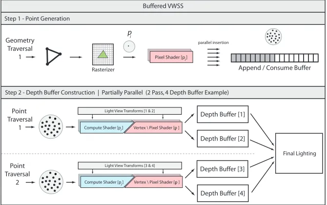
Figure 4.1 Soft shadowing of a 672,927 polygon scene with complex occlusion and dy-namic, skinned geometry at 1080p resolution. Our new VWSS algorithm (middle) computes depth buffers (D) 3.7×faster and the complete image (T) 2.15×faster than Multi-View Rasterization (left). Image quality is compared against a 2,560spp reference and reported using RMSE and HDR-VDP2 per-ceptual heat maps (bottom). VWSS achieves significantly higher numerical and perceptual quality compared to PCSS (right) with a minimal increase in rendering time. . . 34 Figure 4.2 The data flow of buffered VWSS point generation and depth buffer

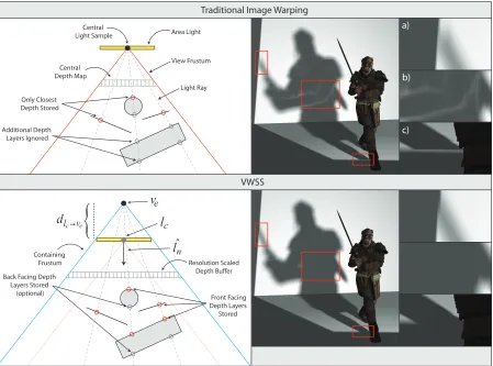
con-struction. In Step 2, each compute (or pixel) shader thread warps a point to multiple depth buffers simultaneously, generating several depth buffers in a single traversal of the point data. . . 36 Figure 4.3 Traditional image warping (top) incorrectly leaks light at areas of

disocclu-sion (b) and shadow boundaries (a,c). These artifacts are eliminated by using VWSS (bottom). . . 37 Figure 4.4 The data flow of unbuffered VWSS. Point generation and depth buffer

con-struction steps are combined into a single execution of the graphics pipeline, as points are streamed from the rasterizer directly to pixel shader threads. . 39 Figure 4.5 The numerical image quality (RMSE) versus performance (ms) for the

War-riors scene (top) and Cliffside scene (bottom) using MVR (red), VWSS (blue), and PCSS (grey). MVR and VWSS use 24, 32, 64, 96, and 128 depth buffers, with quality improving and performance declining as the number of buffers grows. MVR and VWSS reach diminishing quality returns at 96 depth buffers. . . 41 Figure 4.6 The perceptual quality (HDR-VDP2) and performance of VWSS (left) and

PCSS (right) both using 160spp for the Warriors scene (top) and Cliffside scene (bottom). Heatmaps indicate the probability differences between each image and the reference will be perceived. Red areas indicate a higher prob-ability and blue areas indicate lower probprob-ability. . . 42 Figure 4.7 GPU performance of shadowing algorithms as geometric complexity increases

using 24 depth buffers @ 120spp (top) and 128 depth buffers @ 640spp (bot-tom). Multi-View Rasterization (red) exhibits an expected linear rise in ren-dering time as geometric complexity increases. The performance of VWSS (blue) is weakly linked to scene geometry, enabling VWSS to match or exceed PCSS performance (top) and produce a large number of depth buffers in a fraction of the time it takes MVR (bottom). . . 46 Figure 4.8 Top: GPU performance comparison of buffered and unbuffered VWSS

Figure 4.9 Top: The thin sword is not always captured by a 32 sample PCSS blocker search and creates noticeable holes in the sword’s shadow (left). VWSS using an identical number of samples per pixel (middle) has no such failure, delivers quality closer to MVR (right), and retains rendering time similar to PCSS. Bottom: PCSS is unable to handle occluder fusion properly in some scenarios (left), while VWSS shadows are similar to MVR. . . 48 Figure 4.10 Shading modified to emphasize self shadowing. Top: VWSS exhibits self

shadow banding similar to PCSS. Bottom: MVR shows no banding arti-facts, while Normal Offset Depth Biasing applied to VWSS addresses the self shadowing and disconnected contact shadows. . . 49 Figure 4.11 Top: VWSS output for the Volund scene as the area light (yellow) grows.

All area lights use one light sample per two units of light area. Bottom: A close-up comparison of shadows generated by MVR (left) and VWSS (right) reveals very similar results even for large lights. . . 50

Figure 5.1 Left: the view plane is uniformly sampled and the plane of a polygon in the view frustum receives variable sampling under perspective projection. Right: a special case, where the view plane and the polygon have uniform sampling rates when parallel, differing only by a ratio proportional to distance (under perspective projection). . . 52 Figure 5.2 View Independent Rasterization as implemented in the GPU graphics pipeline. 54 Figure 5.3 Left: the minimum point-to-polygon geometric distance dv is found andsmv

is computed. Right: smv determines the polygonal sampling rate for view

independent rasterization. . . 55 Figure 5.4 Sampling type visualizations. a) the original texture mapped geometry. b)

the basic mode displaying a single color for ideal sampling (black), under-sampling (red), and overunder-sampling (cyan). c) an extended visualization mode for oversampling using a single hue and normalized input values. d) a sec-ond extended oversampling mode, using 7 perceptually distinct hues and an additional high constrast color to indicate high oversampling rates. . . 57 Figure 5.5 VIR sampling using the minimum geometric distance from a view center

to each polygon. a) Parallel geometry is sampled ideally. b) Undersampling occurs as the polygon rotates and moves away from the view center. c) Severe undersampling occurs with further rotation and movement towards the view extent. . . 58 Figure 5.6 The geometry of perspective projection distortion. . . 59 Figure 5.7 VIR sampling using Equation 5.3 and the perspective distortion factor w.

Visualization of oversampling is disabled to ease in the detection of under-sampling. By applying the perspective distortion factor when computingsmv,

Figure 5.10 Edge aliasing and undersampling of supra-pixel polygons. Top: the Multi Hue Visualization Mode. Bottom: the oversampling visualization is disabled to ease in the detection of undersampling artifacts. Left: undersampling caused by aliasing between the VIR and view-dependent raster grids. Right: under-sampling is eliminated with conservative rasterization. . . 64 Figure 5.11 An illustration of our optimal perspective distortion factor approximation

strategy. This low polygonal complexity / high projected area example ex-hibits extreme oversampling that is unusual in practice, but is ideal for illus-tration purposes. Left: VIR using the default perspective distortion factor. Notice the high oversampling at the center of the image. Middle: VIR using a less aggressive distortion factor. The number of points generated by VIR is reduced and oversampling is significantly decreased, but undersampling is introduced in the upper right corner of the image. Right: adapting the influ-ence of a point to additional surrounding pixels in areas of high perspective distortion eliminates the undersampling problem while retaining a low overall amount of oversampling across the image. . . 67 Figure 5.12 An illustration of our modified VIR implementation in the graphics pipeline

that generates multiple discrete point-based LoDs while still traversing the geometry only once. . . 68 Figure 5.13 An illustration of Spatial Coherence Point Sample Culling. . . 70

Figure 6.1 As with VWSS, multi-view rendering using View Independent Rasterization restructures depth buffer computation to improve point reuse and paralleliza-tion on GPUs. . . 73 Figure 6.2 A comparison of texel coverage approximations. a) standard polygon

raster-ization, b) point-based rendering, and c) conservative polygon rasterization. . 78 Figure 6.3 A comparison of soft shadowing algorithms. Top: soft shadows rendered using

multi-view rasterization of polygons. Bottom: VIR paired with our GPU Compute parallel view rendering approach. Both methods produce 128 high resolution depth buffers and similar high quality shadow penumbra, but VIR takes only a fraction of the time. . . 79 Figure 6.4 A quality comparison of soft shadows rendered by MVR and VIR. Top Row:

Chapter 1

Introduction

The field of computer graphics is concerned with “the pictorial synthesis of real or imaginary objects from their computer-based models” [27]. Rendering is defined as the process by which the data describing a three dimensional scene is converted into a two dimensional image [66]. Since its inception in the 1960’s, much work in the field of computer graphics has focused on rendering images of astonishing realism by accurately simulating the interaction of light with surfaces composed of nearly every kind of material. This style of rendering is referred to as photorealistic rendering [19]. As the field matured, interactivity in the form of computer games, architectural design tools, advertising, and complex simulations became possible. This form of computer graphics is called real-time rendering, and is primarily concerned with producing images at a rapid rate such that the viewer is unable to perceive individual images, and instead is immersed in an interactive activity [2]. Achieving photorealism requires significant compu-tational power, and the constraints inherent to real-time rendering are typically adversarial to photorealism. As a result, accomplishing photorealism in real-time rendering has become a driving force behind advances in the field of computer graphics. Our research focuses on de-creasing the time required to produce images that include photorealistic effects, thus inde-creasing the achievable visual quality of real-time graphics.

Important visual effects that demand accurate models of light transport, such as soft shad-ows and reflections, are commonly evaluated using multi-dimensional integrals [41]. Solving these integrals in real-time, given the existing computational constraints, is not currently possi-ble. Instead, sampling techniques are employed to approximate a subset of the full light trans-port equation. Sampling techniques are commonly implemented in real-time with GPUs as multiple rasterizations of a scene from differing viewpoints. Algorithms employing this ap-proach are commonly referred to as multi-pass or multi-view [19]. Unfortunately, achieving noise-free results using sample-based approximations requires a large number of samples (or images from unique viewpoints) [49]. Dense sampling of this kind is prohibitively costly for real-time applications, since producing multiple renders of complex geometry reveals a criti-cal limitation in the architecture of existing graphics processors: the throughput optimizations that make GPUs capable of processing millions of polygons also prevent it from leveraging data coherence when synthesizing multiple views. Unlike its parallel processing of vertices and post-rasterization fragments, existing GPU architectures must render views serially and thus parallelize view rendering poorly. The highly detailed and complex input geometry must be re-traversed for every view, missing a critical opportunity to reuse coherent polygonal information and post-rasterization data for similar views. Computing advanced multi-view lighting effects is faster now than before GPUs arrived, but the existing single view design does not realize the full potential of GPUs for accelerated rendering. In this dissertation, we tackle this problem from an algorithmic perspective in order to improve the efficiency of sample generation, increase the number of available samples, and enhance the visual quality of multi-view effects in real-time.

We introduce a GPU accelerated multi-view rendering design that avoids the limitations of GPU-based polygonal rasterization when producing multiple views of a scene. Inspired by the shrinking number of pixels covered by the average polygon, and thus the decreasing importance of polygonal connectivity information [29], we achieve a more flexible rendering design by in-stead using points as the primary multi-view rendering primitive. We improve upon the GPU’s existing serial design by: (1) transforming polygonal surfaces to a point-based representation suitable for rendering multiple views, (2) performing this conversion to points dynamically in real-time using fixed function GPU hardware, and (3) utilizing points to reorganize the struc-ture of computation and enable the efficientparallel rendering of many images. Every stage of our proposed approach executes in a data parallel fashion, such that image generation is now treated like the processing of vertices or fragments in typical polygonal rendering.

qual-ity/performance continuum by: (1) simplifying the multi-view soft shadowing problem using a view-dependent sampling strategy, (2) avoiding common artifacts by tailoring points to many nearby views, and (3) significantly increasing the efficiency of rendering depth buffers by reorga-nizing the rendering workload for coherence. VWSS renders depth buffers up to 13×faster and computes soft shadows over 3× faster than the current state of the art for accurate shadows, on typical real-time dynamic occluder geometry. VWSS exhibits similar performance and less error than existing approximate algorithms of choice, without the serious failure case artifacts that plague single-view approximations. Both the Root Mean Squared Error (RMSE) numer-ical comparison measure and the HDR-VDP2 [53] perceptual image comparison measure rate VWSS’s output as significantly closer to the MVR reference than PCSS.

For lighting effects with less meaningful spatial locality and coherence between views, we introduceView Independent Rasterization (VIR): a fast and flexible method to transform com-plex polygonal meshes into point representations suitable for rendering many views from ar-bitrary viewpoints. By leveraging the decades of optimizations made to fixed function GPU rasterization hardware, while also retaining the flexibility to customize polygon sampling with programmable shaders, VIR presents a new approach to GPU-based view-independent point generation from polygons suitable for real-time applications. We detail how to implement VIR in support of multi-view point-based rendering, compute an appropriate multi-view sampling rate, and mitigate challenging edge cases. We also outline a number of optimization strategies to further improve performance for future practical applications. In our tests, VIR processes two million polygons and generates nearly 600,000 points tailored for 128 views in only 5.48 mil-liseconds. We accelerate the rendering of depth buffers for soft shadows using VIR, and evaluate it using the same methodology as VWSS. The transformation of complex, two million polygon geometry into points and the rendering of 128 high resolution depth buffers is accelerated up to 8× compared to serial MVR. The visual quality of VIR soft shadows is excellent, and even more stable than VWSS due to the view independent point cloud that VIR generates.

Given the promising results of VWSS, VIR, and multi-view point-based rendering on the GPU, we also discuss the application of our algorithms and rendering design beyond shadows, including visual effects such as reflections, defocus blur, and diffuse global illumination. Finally, we discuss the limitations of existing GPU hardware architectures and suggest modifications to evolve them to better support the acceleration of point rendering, the parallelization of image rendering, and ultimately improve visual effects approximated by multi-view sampling algorithms. In summary, the main contributions of this dissertation include:

1. An evaluation of the limitations of the current state of the art in GPU-based multi-view rendering using polygonal and point-based rendering primitives.

of complex visual effects approximated by image-based sampling algorithms.

3. View Warped Soft Shadows: a novel real-time GPU rendering algorithm, based on our multi-view design, that uses a view-dependent point set, accelerates depth buffer gener-ation, casts high quality soft shadows of dynamic geometry from area light sources, and represents a new practical option for applications rendering soft shadows in real-time.

4. View Independent Rasterization: a novel, flexible, real-time GPU-based sampling algo-rithm capable of generating view independent point data sets from polygonal geometry appropriate for an arbitrary number of unique viewpoints.

5. A novel GPU accelerated algorithm leveraging VIR that generates multiple point-based levels of detail (LoD) of polygonal geometry in a single traversal of the source geometry.

6. Detailed performance analyses and visual quality comparisons, using numerical and per-ceptual measures, of our algorithms versus the current state of the art.

7. Point generation and rendering optimization strategies designed for optimal multi-view rendering on existing GPU architectures.

Chapter 2

Background

This chapter provides a brief review of background knowledge and common terminology related to modern graphics hardware architecture, point-based rendering, and the real-time rendering of soft shadows and reflections. Since each of these topics has a rich history, we focus specifically on the subset of terminology and research that is directly relevant to or inspires our work.

Since the introduction of the firstGraphics Processing Unit (GPU) in 1999, the capabilities of dedicated graphics hardware has expanded significantly [62]. Fueled by fierce competition between hardware vendors, the demand for higher graphical complexity in a maturing real-time video games market, and the addition ofGeneral Purpose GPU Computation (GPGPU or GPU Compute) to hardware architectures, the newfound flexibility of modern GPUs simultaneously improved the potential for new algorithmic approaches to classic problems and escalated the nuance-laden difficulty of unlocking that potential as improved performance. We review the common concepts and design elements of modern GPU architectures to provide a universal lan-guage and context for reasoning about algorithmic performance on modern hardware platforms. Point-Based Rendering challenges the universally accepted use of polygons as the primary rendering primitive by instead modeling objects as a collection of infinitesimal three-dimensional points [50]. The use of points as the primary rendering primitive has been demonstrated in offline systems as a viable strategy to accelerate the rendering of complex effects including soft shadows and reflections [29]. Leveraging points as a more efficient surface representation serves as a foundational concept in our approach to accelerate challengingreal-time workloads. We review concepts and terminology, discuss common challenges, and identify relevant open problems associated with point rendering.

Figure 2.1: A conceptual representation of modern GPU architectures [39].Left: the common shader core.Right: the GPU Compute threading model. Thread groups are shown in orange.

multiple views are still commonly employed to approximate these integrals for challenging visual effects [28, 32, 33].Soft shadows and reflections are two such effects, where each serial render increases the effective scene complexity and decreases data coherence. As a result, these effects are ideal test cases for our multi-view point-based rendering approach. We review concepts and terminology associated with existing accurate and approximate approaches for rendering soft shadows and reflections.

2.1

Architecture of Modern Graphics Processors

The design and implementation of our work is informed by the existing capabilities of modern graphics processors. Conceptually, a GPU can be understood in two ways: (1) as an array of small processors that manipulate large amounts of similar data in parallel; or (2) as a sequential set of pipelined stages, each executing in parallel, responsible for specialized predetermined tasks when manipulating polygonal data to render images.

InputM

Resou

rces Output

Resou

rces

Output

Resou

rces

Input

Assembler ShaderVertex ShaderHull Tessellator DomainShader GeometryShader

StreamM Output

Rasterizer _ShaderPixel Output_Merger

Figure 2.2: A conceptual model of the GPU graphics pipeline [39]. Fixed function stages are shown in green and programmable stages are in blue.

single GPU processor. Shown in orange, threads are organized into conceptual groups. Thread groups are then sent to the GPU, scheduled, and executed in vendor defined quantities (32-thread warps on NVIDIA and 64-thread wavefronts on AMD). User authored programs that execute using this threading model are typically referred to as Compute shaders.

The Programmable Graphics Pipeline

Figure 5.2 depicts the stages of the graphics pipeline, each of which receives input data from the previous stage, performs specialized processing, and outputs result data to the next stage. The flexibility introduced by the common shader core also improved the existing graphics pipeline. There are now two types of graphics pipeline stages. Fixed function stages perform specific tasks using purpose-built hardware units, but can only be configured through predetermined parameters. The rasterizer is an example of a fixed function stage.Programmable stages perform a wider range of tasks by executing user authored shader programs based on the common shader core. By replacing previously fixed-function stages (Vertex, Pixel) with programmable shader stages, as well as adding entirely new stages (Tessellation, Geometry), modern architectures avoid performance bottlenecks by adapting available processing resources to varying workload demands on the fly. Currently, there are five programmable graphics pipeline stages. Each stage is responsible for a unique type of parallel processing.

Unlike the vertex shader, however, the control point function can create up to a maximum of 32 new control points per input patch. The patch constant function is executed once per input patch and produces the tessellation factors. The fixed function tessellator accepts the tessellation factors, subdivides the input patch, and outputs a set of weights representing the post-tessellation structure of the input patch. These weights are tailored to the input topology; therefore, a set of barycentric coordinates are produced for triangular patches. The domain shader is the final stage of the tessellation pipeline and is responsible for processing post-tessellation vertices output by the tessellator. The domain shader operates as a post-post-tessellation vertex shader, but unlike the vertex shader it has access to all control points and patch constant information generated by the hull shader.

The last programmable stage before rasterization is the geometry shader stage. In this optional stage, vertex information for the entire primitive, as well as adjacent primitives, is available. The geometry shader includes unique functionality for manipulating primitives of varying topology, the ability to create new geometry of arbitrary topology on the fly, the ability to store (orstream out) vertex data pre-rasterization, and the ability to designate primitives be rasterized to multiple different target images. Creating new geometry in the graphics pipeline is referred to as amplification. The geometry shader guarantees the output order of primitives matches the input order, which can severely affect performance [2].

The final programmable stage of the graphics pipeline is the pixel shader stage. The pixel shader stage, whose name is somewhat of a misnomer, processes polygon fragments produced by the rasterizer. Lighting, shading, and post-processing effects are commonly implemented in pixel shader programs. Importantly, the pixel shader stage includes extended functionality available to compute shaders, but not available to other graphics pipeline stages. This enables pixel shaders to perform a wider set of advanced operations at the end of the graphics pipeline, including image processing algorithms such as Screen Space Ambient Occlusion (SSAO) [59] and approximate motion blur effects using velocity buffers [2].

Conservative Rasterization

Conservative Rasterization Standard Rasterization

Figure 2.3: The results of standard rasterization and overestimating conservative rasterization. For each method, pixels that produce samples for the triangle are colored grey.

a pixel, while underestimating requires the pixel’s entire area be contained within a polygon. The overestimating method is implied when the specific type of conservative rasterization is not specified. Overestimating conservative rasterization is shown on the right side of Figure 2.3.

Memory Structures

Modern GPU architectures include several memory structures for data storage. Two dimensional arrays used for storing image data are referred to as textures. The individual pixels of textures are known astexels. Textures can be designated as input to any programmable stage. Textures written by the graphics pipeline are referred to as render targets. To avoid undefined behavior from memory contention, a texture cannot simultaneously be a shader input and a render target. One dimensional arrays used for storing data of arbitrary format are called buffers.Append / Consume buffers are a stack-like buffer storage variation that maintains an internal atomic counter enabling optimized parallel insertion and deletion operations [39]. Append / Consume buffers were initially used for GPU-based particle systems, but are also useful when performing point-based rendering.

2.2

Point-Based Rendering

Point-Based Rendering introduces an alternative to the ubiquitous use of polygons as the pri-mary rendering primitive by modeling three-dimensional objects as a collection of infinitesimal three-dimensional points. The motivation for this change is based on the insight that a polyg-onal surface representation is not the most efficient when a polygon covers only a single pixel of an output image [50]. Understanding the design of rendering algorithms further reveals the relationship which makes point-based rendering useful.

Rendering algorithms are broadly classified into two categories based on how object visibility is determined: (1) image-order and (2) object-order [29]. Image-order algorithms use a gather approach where each pixel of an image searches the scene for the closest intersecting geometric primitive. Ray tracing is an example of an image-order algorithm [85].Object-order algorithms use a scatter strategy by examining each geometric primitive and determining which pixels are intersected. Rasterization and the Z-buffer are common object-order algorithms [12]. The efficiency of image-order and object-order algorithms is determined by the quantity of work and the coherence of data within each step of the algorithm. Historically, computer generated images have consisted of many more pixels than geometric primitives. In this scenario, each geometric primitive covers many pixels and exhibits high coherence during object-order traversal. As a result, object-order algorithms have received dedicated hardware acceleration and significant optimization efforts.

The object-order optimization of GPU architectures resulted in extremely high polygon throughput, and spurred a rapid increase in the number of geometric primitives used when rendering images. In the past decade, the geometric complexity of interactive applications has increased to match or even exceed the number of output pixels [23]. Compounding this increase in complexity, the demand for more advanced lighting effects, such as soft shadows or reflec-tions, in real-time applications became higher than ever. Critically, these effects require more information than what is directly available in any single viewpoint. Existing GPU architectures implement distributed rasterization algorithms to sample geometric primitives for a single view at a time. These samples are calledview-dependent. As a result, sampling scene geometry from multiple views or directions using the GPU’s rasterizer must be performed serially. This causes multiple traversals of the complex geometry, a decrease in the coherence of the object-order algorithm, and a linear increase in the GPU’s triangle setup and rasterization tasks.

Figure 2.4: Point-based rendering as illustrated in [29]. Left: Naive forward mapping of points. Right: Splatting distributes a point’s contribution across an area of nearby pixels.

by a factor of two requires four times more points [29], more efficient representations have been proposed which approximate the surface using a small circular or elliptical area around the point sample [65]. To render an image, the point sample representation is forward mapped to the raster grid in a process known assplatting [91, 83]. This is illustrated in Figure 2.4. Since each point contains all required rendering information, operations performed by GPU hardware to interpolate values across polygons, such as clipping, scan conversion, and texture mapping, are no longer necessary. A view-independent point-based representation also has an automatic level of detail (LOD), since a surface is more coarsely represented by simply reducing the num-ber of points [50]. Recently, game developers have presented experimental fully programmable point-based graphics systems for interactive games [24]. Figure 2.5 shows pre-production results from Media Molecule’s Playstation©4 title “Dreams”. Various artistic effects are achieved by varying the point sampling density and the pixel area of a point’s influence during splatting.

a) b) c) d)

Figure 2.6: The pull-push algorithm from [30]. a) Original image. b) An incomplete image with gaps. c) Pull Phase: creates lower resolution approximations. d) Push Phase: uses the low resolution images to reconstruct a complete, but blurred result.

Challenges and Open Problems

The potential efficiency improvements and simplicity of a point-based representation are not without drawbacks. Since points no longer store polygonal connectivity information, it is pos-sible for point rendered images to lack complete information about surfaces when point data is not sufficiently dense for the target image’s resolution [29]. Illustrated by Figure 2.6b, this causes visible “holes” where some data for a surface is not present in the image. The hole-free representation of a surface for an arbitrary view is referred to aswatertightrendering. Achieving watertight rendering is the primary challenge associated with point-based rendering. Although it has been shown that the watertight sampling density of a surface can be computed by using the determinant of the Jacobian of a unit-sized patch transformed to screen space [50], this approach is still challenging to accomplish efficiently on existing GPU architectures.

Until now, there have been two main approaches to achieving watertight point-based ren-dering on GPUs: (1) process highly dense, oversampled point sets, or (2) augment low density point sets with smarter splatting logic and hole-filling post processes [55]. Historically, limited storage and memory bandwidth have made high density point solutions infeasible for practical real-time use. Consequently, much of the existing research in point rendering focuses on using low density point sets rendered using various techniques, such as Elliptical Weighted Aver-age (EWA) filtering [91], that construct a resampling kernel during splatting [45]. A common post-process hole-filling algorithm is referred to aspull-push [30]. This approach produces lower resolution approximations of the final image and then uses those approximations to fill gaps.

2.3

Rendering Soft Shadows in Real Time

Shadows are perceptually important elements of visual scenes [44]. Visual cues encoded in shadows were identified as early as Renaissance painters and studied more recently by cogni-tive psychologists. Shadows provide static and dynamic visual clues about the location, shape, and arrangement of objects in an environment, as well as various characteristics about light sources [52]. The shadowing effect is created by objects preventing light energy, or photons, from reaching other objects in an environment.

The anatomy of a shadow is illustrated in Figure 2.7. Objects that block photons are referred to asoccluders orshadow casters. Objects on which shadows are cast are referred to asreceivers [22]. It is common for an object to simultaneously be both an occluder and a receiver. The shadow created by an occluder consists of a fully unlit region, theumbra, as well as a partially lit region, the penumbra. The penumbra is a gradient from completely unlit to lit, starting at the edge of the umbra and extending outward [20]. The penumbra’s shape is produced by a combination of several factors including: (1) occluder shape; (2) occluder proximity to the receiver; (3) light source shape; and (4) light source proximity to the occluder. An important visual effect of the penumbra is called contact hardening [22]. As an occluder gets closer to a receiver the shadow penumbra width decreases in size. This relationship causes the shadow to appear “harder” as the occluder gets closer to making contact with a receiver.

penumbra umbra

occluder

receiver

contact hardening

Point Lights

Early attempts at rendering shadows in real time modeled light sources as infinitesimal points, known as point lights. Photons emitted from point lights are modeled as rays traveling unim-peded from the point light source to the closest occluding surface. Image-based implementations of point light shadows store light rays as depth values in a discrete two dimensional array, called adepth buffer ordepth map. Shadows are then computed by comparing the distance to a point in the eye’s view against the distance stored in the depth buffer for that point. This process is commonly known as shadow mapping [86] and is shown in Figure 2.8. When using a point light source, the shadow computation ignores the possibility of penumbra. This is referred to ashard shadowing due to the binary shadows it produces; where areas are either “in” shadow or “out” of shadow. Often the sampling rate of the depth buffer and eye’s view do not match. This difference is known asshadow aliasing and manifests visually as sharp, often jagged, edges such as those shown in Figure 2.8. Recent advanced algorithms have resolved a majority of the aliasing artifacts which plague hard shadowing approaches [48] [89]; however, these methods are computationally expensive and ultimately still lack shadow penumbra.

depth buffer

Area Lights

Nearly all light sources in the physical world emit photons across some area in three-dimensional space. As a result, the point light source used in hard shadowing algorithms is not sufficient to produce accurate shadows [22]. More accurate algorithms model light sources as planes with non-zero area, called area lights. The geometric relationship of shadows cast from area light sources is illustrated in Figure 2.9. While still an approximation, shadows computed from area lights exhibit convincing shadow penumbra. Due to the soft edges exhibited by the penumbra, this type of shadow rendering is often referred to as soft shadowing.

Figure 2.9: Left: The geometry of shadows cast from an area light. Right: a large area light increases the size of the penumbra and decreases the size of the umbra [21].

Accurate Methods

The primary task ofsoft shadowing algorithms is to determine the proportion of an area light visible to a receiving surface. This proportion is known as the visibility factor [22]. Despite the massive increase in parallel processing capability over the past decade, this area visibility problem remains difficult due tooccluder fusion: the non-trivial interaction of multiple occluding surfaces preventing the individual processing and combination of occlusion data [20].

Figure 2.10: Left: accurate shadow penumbra produced by distributed ray tracing [15]. Right-Top: soft shadow convergence after 1, 3, 7, 20, and 256 frames using temporal coherence. Right-Bottom: Temporal reprojection used to improve the speed of convergence [72].

requirement of multiple traversals of occluder geometry still prevents real-time performance in most scenarios. To achieve acceptable quality with rasterization, anywhere from 256 to 1,024 depth buffers may be required to achieve convergence [22].

Temporal Methods

Reference PCSS Variance Shadow Mapping

Figure 2.11: Left: compared to the reference, PCSS produces soft shadows that are too large [21]. Right: Variance Shadow Mapping leaks light into the umbra even in a basic situation [2].

Approximate Methods

Most existing real-time applications abandon accurate methods for approximations that produce flawed but plausible results. The fastest approximate soft shadowing algorithms accept a single depth buffer as input, and even work well in specific cases, but often fail in other common situations due to the complex behavior of the penumbra. For this reason, no single approximate method is best for all scenarios.

Early soft shadowing approximations stemmed from attempts to anti-alias the boundary of a hard shadow.Percentage Closer Filtering (PCF) is commonly used to filter depth buffers by comparing depth texel values with the depth of the surface being rendered [67]. Statistics based methods, such as Variance [18], Convolution [3], and Exponential Shadow Mapping [4] apply various mathematical techniques that alter the values stored in depth buffers to achieve the goal of representing a range of values. Shown on the right of Figure 2.11, statistics based filtering methods erroneously leak light into the shadow umbra, have fixed size penumbra, and do not reproduce contact hardening effects.

Imperfect Shadow Mapping

Imperfect Shadow Mapping (ISM) approximates visibility for indirect illumination using many low resolution depth buffers, generated by splatting an approximate point-based representation of the scene geometry [68]. Due to the low frequency characteristics of indirect illumination, the errors caused by ISM’s low resolution, approximate visibility data are largely unnoticeable. ISM generates its view-independent point representation either offline or at run-time using GPU tessellation hardware [5]. Figure 2.12 illustrates the steps to accomplish ISM splatting with GPU tessellation point generation at runtime. The number of points generated by the hardware tessellator is determined by the triangle’s surface area. To achieve real-time performance, ISM constructs depth buffers by splatting each point to one randomly chosen depth buffer. This crude approximation creates incomplete depth buffers, which are hole-filled by the pull-push post-processing algorithm discussed earlier.

Figure 2.12: A diagram from [5] of the steps in the graphics pipeline to implement ISM splatting with points generated by GPU tessellation.

ISM has several drawbacks for real-time applications. Although the use of the GPU tes-sellation pipeline to generate points is clever, it introduces efficiency problems for tessellated dynamic objects. In this case, the object must be (1) traversed and tessellated, (2) stored to GPU memory, and (3) re-traversed and transformed into points. Additionally, ISM is not ap-propriate to render shadows cast by direct light sources, since it is unable to capture the high frequency fine details required to avoid undesirable artifacts. Finally, post-processing hundreds of higher resolution depth maps using pull-push is a costly, bandwidth intensive operation.

2.4

Rendering Reflections in Real Time

To achieve realistic images, the interaction between light energy and each rendered surface is modeled. When photons interact with a surface they either: (1) scatter into the surface, known as transmission, or (2) scatter away from the surface, which is referred to asreflection. The general mathematical model of light scattering is known as the bidirectional scattering distribution function (BSDF). When focusing on just reflection, the ratio of incoming to outgoing energy is described mathematically by thebidirectional reflectance distribution function (BRDF) [2].

Planar Reflections

The left side of Figure 2.13 illustrates the geometry of reflection for planar surfaces. It demon-strates the law of reflection which states, “the angle of incidence (θi) is equal to the angle of

reflection (θr)” [2]. Due to this relationship, planar surfaces constitute a special case where

photons reaching the eye from reflected surfaces are identical to photons arriving along the incident ray for geometry which has been physically reflected about the surface plane.

Conveniently, this relationship can be exploited by image-based rendering techniques, mak-ing planar surfaces easier and more efficient to render than more complex cases [2]. Reflected objects are simply rendered twice, where the geometry and relevant light sources are trans-formed about the reflection plane during the second render. In the shading step for the planar reflector, the reflection image is sampled when computing incoming radiance. The right side of Figure 2.13 provides an example of this technique from the real-time racing simulation game “Project Cars”. Notice the high quality reflection of the car and background building in the fore-ground water puddles. Given the availability of dense screen-space data structures such as the

θr θi

G-Buffer [69], aggressive approximations of planar reflections have been presented [79]. How-ever, due to the limited data available in these view specific data structures, these techniques often still require fall-back strategies [78].

Non-Planar and Environment Mapped Reflections

Reflections produced by non-planar objects are unable to use the simplifying assumptions which make planar reflections efficient. Consequently, different techniques have been developed that store incoming radiance values in look-up tables, calledenvironment maps [2]. The concept of environment mapping was first introduced using a longitude / latitude system to map reflection vectors into polar coordinates [7]. The process of environment mapping is depicted on the left side of Figure 2.14 and contains the following steps:

1. Generate or load an image representing the environment.

2. Compute the surface normal and reflection direction for each visible surface.

3. Use the reflection direction to compute an index into the environment map image.

4. Sample and use data from the environment map image to represent incoming radiance.

Figure 2.14: Left: the environment mapping process [2]. Right: The longitude / latitude system used in Blinn and Newell’s original environment mapping scheme [2].

N

M

Q S P

O

M O P

N

S

Q

Figure 2.15: Cubic environment mapping renders the scene to each axis-align face of a cube. Modern hardware supports sampling this custom texture using a 3-component direction vector. Right: an example of a cubic environment map from [28].

Chapter 3

Multi-View Point-Based Rendering

in Real-Time

This chapter introduces the multi-view point-based rendering framework that serves as the conceptual foundation for the research presented in subsequent chapters. First, we describe the motivation behind our point-based strategy. Next, we introduce an algorithmic framework for efficiently generating points from polygonal geometry in real time and parallelizing multi-view image rendering. We detail how our approach realizes untapped potential of existing GPUs by avoiding the inefficiencies of existing rendering methods, while laying the groundwork for future hardware opportunities to further optimize point-rendering for complex visual effects.

3.1

Motivation

The accurate simulation of light requires evaluating complex multi-dimensional integrals for each visible surface [41]. Sampling techniques are commonly employed to approximate these integrals; however, effects such as soft shadows, defocus blur, and reflections typically require a large number of samples to produce noise-free results [49]. Since dense sampling is prohibitively costly for real-time applications, filtering approaches instead attempt to reduce noise by locally sharing information between a small set of samples [77]. Despite achieving acceptable results in many cases, filtering approaches are ultimately limited by the quantity of input samples they operate on. As a result, we are motivated to improve the efficiency of sample generation to increase the number of available samples, and enhance the visual quality of all approaches.

support of the desired effect. A depth buffer used in shadow mapping and the faces of a cube map used in environment mapping are examples. These samples are distinctly different than polygonal samples, which are discrete representations of geometric surfaces as opposed to the content of an entire view. At the moment, the fastest method of generating polygonal samples is GPU-based rasterization. Our algorithms utilize the rasterizer for its decades of optimized silicon; however, our general approach accommodates any polygonal sampling method should another prove more capable as hardware architectures evolve (for example, procedural sampling of geometry or ray tracing).

3.1.1 Limitations of Existing Methods

To accelerate multi-view image rendering, we first identify the inefficiencies present in the design of existing rendering architectures. Currently, fixed function rasterization hardware is highly optimized to produce a watertight rendering of polygonal surfaces for a single view. Geometry is streamed through a set of parallel pipelines, where processing is performed for many polygons concurrently. Each input polygon is (1) transformed into the target view, (2) sampled appropriately for the given image resolution, and (3) stored as an image. This design enables extremely high polygon throughput while requiring relatively modest caching structures; however, its bias of throughput over coherence is also a severe limitation. In multi-view scenarios where several images contain large amounts of similar data, the cost of being unable to keep previously processed data cached for fast retrieval during subsequent executions is a significant limiting factor. Unlike its parallel processing of vertices and post-rasterization fragments, this existing design must render views serially and thusparallelizes view rendering poorly. Shown in Figure 3.1, input geometry must be traversed for every view, missing a critical opportunity to reuse coherent polygonal information and post-rasterization data for similar views.

1 Transform [1] Sample Image [1]

Final Image

2 Transform [2] Image [2]

n Transform [n] Image [n]

GPU Executions

Input Polygons

View Transform

Accumulation or Averaging

Sample

Sample

Figure 3.2: Multi-View Rasterization of soft shadows from [37]. Top: depth buffers rendered from varying light sample positions on the area light. Bottom-Left: the area light, occluder, and receiver. Middle: multiple hard shadows produced by only 4 depth buffers. Bottom-Right: the fully resolved soft shadow using 256 depth buffers.

As a thought experiment, consider the case of rendering soft shadows from an area light source using Multi-View Rasterization. Randomly positioned points are distributed across an area light. MVR uses each of these light samples as an eye location and rasterizes geometry between the eye and the receiver to produce many depth buffers. To compute the soft shadow visibility factor, MVR averages the results of shadow mapping using each depth buffer. The bottom row of Figure 3.2 illustrates this scenario.

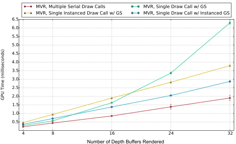
Number of Depth Buffers Rendered

Figure 3.3: A comparison of triangle rasterization implementations rendering multiple depth buffers of a 240,186 polygon character. Rasterizing multiple depth buffers in a single graph-ics pipeline execution is often slower than serial multi-pass methods due to memory access challenges and limitations of the Geometry Shader.

3.2

A Multi-View Rendering Design

Motivated by these limitations, we seek a more efficient – yet still accurate – alternative to polygonal rasterization that exploits today’s GPU hardware. Inspired by the shrinking number of pixels covered by the average polygon, and thus the decreasing importance of polygonal connectivity information [29], we achieve a more flexible rendering design by instead using points as the primary multi-view rendering primitive. The atomic nature of points is a natural fit for the Same Instruction Multiple Data (SIMD) nature of the GPU’s processor array, especially outside of the traditional graphics pipeline when using GPU Compute.

Since the vast majority of real-time content, authoring tools, and practitioner skills are reliant on polygonal primitives, it is imperative our new rendering design support existing content creation standards without significant modification. To achieve this, scene content is authored as polygons and transformed into a point representation at runtime. By deferring the conversion of assets into points until runtime, our design supports all existing content, gains the flexibility to tailor generated point primitives to the most appropriate representation for the specific rendering goal, and enables a reorganization of the three rendering steps described in Section 3.1.1. Our point-based multi-view rendering design is illustrated below in Figure 3.4.

1 Calculate Multi-View Sample Sampling Rates

Final Image

2 Splat Image [2]

Image [n] GPU

Executions Input

Image [1]

Point Representation

Dynamic Point Generation

Parallel Image Rendering

Figure 3.4: Our point-based multi-view rendering design. Input polygons are converted to point primitives at runtime and then multiple images are rendered in parallel using the points.

Currently, point-based rendering is rarely used for real-time multi-view effects since 1)dense point sets appropriate for every possible view cannot be regenerated in real-time for animation, nor be rendered to all views within real time frame budgets; while 2) sparse point sets require elaborate splatting and reconstruction algorithms that do not parallelize effectively on existing GPUs, and ultimately suffer from low quality approximations of the original geometry. Existing graphics hardware solves direct illumination by coupling dense sampling tailored to the current view with extremely simple reconstruction that parallelizes well, fully exploiting the GPU’s raw power. Inspired by this approach, our design solves for multi-view approximated indirect illumination effects by enabling ahigh density point set tailored per frameto the current multi-view configuration, coupled with relativelysimple reconstruction kernels.

3.2.1 Generating Points from Polygons

At the turn of the century, the introduction of 3D laser scanning technology re-invigorated interest in point-based rendering methods [29]. The acquisition of highly detailed point sets from real-world objects became possible, and fueled research in the simplification and efficient rendering of incredibly dense point data sets [65, 91, 8]. We refer to point acquisition from 3D scanning asstatic point generation, since points are produced by an offline pre-processing step. Detailed surveys of static point generation [29] and rendering [45] are available. Despite the exciting ability to accurately and efficiently render real objects with exceptional detail, render-ing static point sets is impractical and undesirable for many real-time applications. For these applications points must be generated at runtime, typically from polygonal representations. We refer to this process as dynamic point generation.

from triangles in the geometry stage of the graphics pipeline [5], but is limited by a relatively simplistic point generation heuristic.

A primary focus of this dissertation is multi-view dynamic point generation for various effects that exhibit different levels of multi-view coherence. To cover these topics in detail, we present new view-dependent and view-independent dynamic point generation approaches in the chapters that follow. Chapter 4 details a multi-view view-dependent algorithm that enables up to a 13× performance improvement in depth buffer rendering and 3× improvement to overall soft shadow rendering. In Chapter 5, we introduce a new view-independent algorithm, View Independent Rasterization, that leverages fast fixed-function rasterization hardware to sample polygons at runtime without many of the downsides of existing view-independent methods. We then discuss how to apply View Independent Rasterization to multi-view effects such as soft shadows, defocus blur, and environment mapped reflections. Each of these novel point generation techniques employs a parallel image rendering approach that we describe next.

3.2.2 Parallel Image Rendering

After point generation, images are rendered using the point representation. Unlike the multi-view rasterization process illustrated in Figure 3.1, multiple images are constructed in a single execution of the GPU. This process is the second step in our multi-view point-based rendering framework and is shown in Figure 3.5 below:

Final Image

2 Splat Image [2]

Image [n] Image [1]

1 Calculate Multi-View Sample

Sampling Rates

Figure 3.5: Images constructed in parallel using generated points in a single GPU execution.

Lower Performance Lower Memory Usage

Higher Performance Higher Memory Usage

Serial

Methods 1- 4 Methods 5 - 8 Methods 9, 10

Fully Parallel

Partially Parallel

Figure 3.6: Multi-view point rendering exists on a continuum from serial, to partially parallel, to fully parallel execution per traversal of the point data.

point’s world-space location, and then for each view, applying the corresponding view-projection matrix, snapping the projected location to the nearest neighbor texel in the view’s buffer, and performing z-buffering. Atomic functions resolve race conditions created by multiple points projecting to the same texel. Although this approach implicitly associates a point sample’s area of influence with the extent of a single texel, gaps in constructed images are avoided because of the sampling density calculations completed during dynamic point generation. Other more advanced splatting techniques from the point rendering literature [91] could be employed here; however, they are less efficient and usually unnecessary.

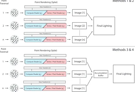
Due to the rapid evolution of graphics architectures towards generalized computation, ex-isting hardware includes a surprising number of ways to accomplish parallel image rendering with points, using either the graphics pipeline or GPU compute. We classify and compare multi-view point rendering approaches based on the amount of parallelism they achieve during each traversal of the point data. Shown in Figure 3.6, image rendering exists on a continuum, and is accomplish by either producing one image per traversal (serial), 2) multiple images per traversal(partially parallel), or 3) all images per traversal(fully parallel). Based on the available feature set of existing GPU hardware, there are no fewer than ten ways to render all points to all images. We detail these implementation options below:

Methods 1 - 4: Serial

Final Lighting Point Rendering (Splat)

Image [1]

Image [2]

Image [n] 2

n

Compute Shader [p ] _i Vertex / Pixel Shader [p ]_i Point

Traversal

1

Compute Shader [p ] _i Vertex / Pixel Shader [p ]_i

Compute Shader [p ] _i Vertex / Pixel Shader [p ]_i

Methods 1 & 2

Methods 3 & 4

View Transform [1]

View Transform [2]

View Transform [n]

Final Lighting Point Rendering (Splat)

Accumulation Buffer Image [1] Image [1] Image [1] 2 n

Compute Shader [p ] _i Vertex / Pixel Shader [p ]_i Point

Traversal

1

Compute Shader [p ] _i Vertex / Pixel Shader [p ]_i

Compute Shader [p ] _i Vertex / Pixel Shader [p ]_i

View Transform [1]

View Transform [2]

View Transform [n]

Figure 3.7: Serial multi-view point rendering traverses point data once for each rendered image. Top: A unique intermediate image buffer per traversal. Bottom: Employing an accumulation buffer decreases memory use and distributes shading memory bandwidth over traversals.

memory use, and distributes shading memory bandwidth over several passes. This method, illustrated on the bottom of Figure 3.7, allows serial rendering passes to reuse the same image buffer at the cost of increasing overall memory traffic.

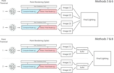
Methods 5 - 8: Partially Parallel

Large quantities of fast global video memory (12 GB and rising) are now available on existing graphics hardware. Illustrated in Figure 3.8, this change in storage capacity makes rendering more than one intermediate image per traversal practical. Rendering multiple images simultane-ously reduces the total memory traffic incurred by loading points and increases memory access coherence during point rendering. As with serial rendering, a partially parallel strategy can also bound memory usage by modifying point traversal passes with an accumulation buffer. When implementing this method in the graphics pipeline, points are loaded in the Vertex shader, but projection is deferred until either the Geometry or Pixel shader stages. This important change prevents the rasterizer from culling points that project outside any single view.

Image [1]

Image [2]

Image [3]

Image [4]

Final Lighting Point Rendering (Splat)

Point Traversal

Compute Shader [p ] _i Vertex / Pixel Shader [p ]_i 1

Compute Shader [p ] _i Vertex / Pixel Shader [p ]_i 2 Accumulation Buffer Image [1] Image [2] Accumulation Buffer Image [1] Image [2] Final Lighting

Methods 7 & 8

Point Rendering (Splat) Point

Traversal

Compute Shader [p ] _i Vertex / Pixel Shader [p ]_i 1

Compute Shader [p ] _i Vertex / Pixel Shader [p ]_i 2

Methods 5 & 6

View Transforms [1 & 2]

View Transforms [3 & 4] View Transforms [1 & 2]

View Transforms [3 & 4]

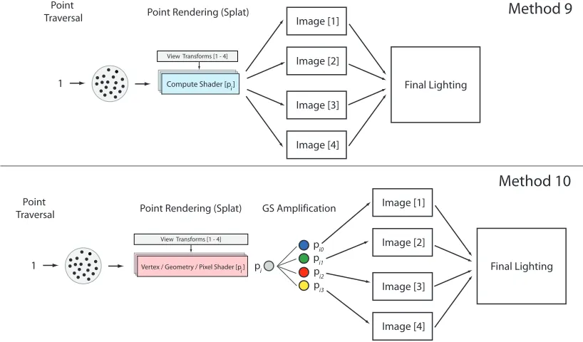
Methods 9 & 10: Fully Parallel

Illustrated in Figure 3.9, a fully parallel point rendering approach constructs all intermediate images in a single traversal of the point data. In this method, the memory bandwidth incurred from loading points is minimized and coherence during point rendering is maximized. GPU memory bandwidth ultimately limits the number of images that are efficiently rendered by each point data traversal; therefore, the fully parallel method is not appropriate in memory bandwidth limited environments (legacy and low-end GPUs).

Unlike previous methods, implementations of this method differ due to limitations in the hardware’s architecture. GPU compute is able to render any number of intermediate views simultaneously, but is not able to use the texture sampling hardware for mipmapping and filtering. When using the graphics pipeline and the Geometry Shader, each input point is copied for each output view and rasterized to the corresponding image. The Geometry Shader is restricted to 32 copies per execution. If the number of output views exceeds 32, the graphics pipeline implementation must fallback to partially parallel execution. The Geometry Shader also has well known performance problems when performing data amplification [2]; however, the Pixel Shader stage later in the pipeline is capable of using texture sampling hardware.

Final Image Splat

Image [1]

Image [n] Image [0]

0 Vertex _Shader

Geometry Shader Rasterizer Image [1] Image [2] Image [3] Image [4] Final Lighting Point Rendering (Splat)

Point Traversal

Compute Shader [p ] _i 1 Method 9 Method 10 1 Image [1] Image [2] Image [3] Image [4] Final Lighting GS Amplification

Point Rendering (Splat) Point

Traversal

Vertex / Geometry / Pixel Shader [p ] _i

p_i0 p_i1 p_i2 pi3

p_i

View Transforms [1 - 4]

View Transforms [1 - 4]

Figure 3.9: Fully parallel multi-view point rendering produces all intermediate images in a single point data traversal. Top: Any number of output images is possible with GPU Compute. Bottom: Implementation in the graphics pipeline is more complex and involves more shader stages. The Geometry Shader creates copies of the original point to render each image.

Chapter 4

View Warped Multi-View Soft

Shadows for Area Lights

In this chapter, we apply our multi-view point-based rendering concept to an important visual effect: soft shadows cast from area lights. As we discussed in Chapter 2, shadows provide impor-tant perceptual cues. These cues are even stronger when shadows exhibit natural characteristics such as penumbras [52]. Recent advances in the precomputation and compression of visibility data for static occluders has enabled real-time shadowing algorithms to focus on the subset of occluders and lights that are animated or otherwise dynamic [70, 61]. For these dynamic ele-ments, Multi-View Rasterization (MVR) is the best proxy for a ground truth solution that real time applications can consider to accurately reproduce soft shadows; however, its requirement of multiple traversals of occluder geometry prevents real-time performance [22].