Spatial Variation and Interpolation of Wind Speed Statistics and Its Implication in Design Wind Load

(1)

Western University Western University

Scholarship@Western

Electronic Thesis and Dissertation Repository

4-22-2013 12:00 AM

Spatial Variation and Interpolation of Wind Speed Statistics and

Its Implication in Design Wind Load

Wei Ye

The University of Western Ontario

Supervisor

Dr. Hanping Hong

The University of Western Ontario Joint Supervisor Dr. Jinfei Wang

The University of Western Ontario

Graduate Program in Civil and Environmental Engineering

A thesis submitted in partial fulfillment of the requirements for the degree in Doctor of Philosophy

Follow this and additional works at: https://ir.lib.uwo.ca/etd

Part of the Civil and Environmental Engineering Commons

Recommended Citation Recommended Citation

Ye, Wei, "Spatial Variation and Interpolation of Wind Speed Statistics and Its Implication in Design Wind Load" (2013). Electronic Thesis and Dissertation Repository. 1254.

https://ir.lib.uwo.ca/etd/1254

This Dissertation/Thesis is brought to you for free and open access by Scholarship@Western. It has been accepted for inclusion in Electronic Thesis and Dissertation Repository by an authorized administrator of

(2)

SPATIAL VARIATION AND INTERPOLATION OF WIND SPEED STATISTICS AND ITS IMPLICATION IN DESIGN WIND LOAD

(Thesis format: Integrated Article)

by

Wei Ye

Graduate Program in Engineering Science Department of Civil and Environmental Engineering

A thesis submitted in partial fulfillment of the requirements for the degree of

Doctor of Philosophy

The School of Graduate and Postdoctoral Studies The University of Western Ontario

London, Ontario, Canada

(3)

ii

ABSTRACT

Consideration of wind load is important for design of engineered structures. Codification of wind

load for structural design requires the estimation of the quantiles or return period values of the

annual maximum wind speed. The extreme wind speeds are estimated based on the measured

wind records at different meteorological stations and affected by the length of the wind record

(i.e., sample size) and other factors such as the surrounding terrain and so on. This study is

focused on 1) the spatial interpolation of wind speed statistics, 2) the potential of using regional

frequency analysis in estimating the extreme wind speed, and 3) the reliability of designed

structure at sites with and without sample size effects.

For the spatial interpolation, both code recommended values of the wind speed as well as those

based on at-site analysis are used, and commonly used spatial interpolation methods including 8

deterministic methods and 6 geostatistical methods have been applied. The preferred methods

for each data set are determined based on the (leave-one-out) cross validation analyses. It is

shown that the preferred method depends on the considered data set; the use of the ordinary

kriging is preferred if a single method is to be selected for all considered data sets.

The historical wind records and available meteorological stations are often short and insufficient

or unavailable, and the limited sample size will cause the uncertainty in the estimated quantiles.

To deal with the data insufficiency in the wind speed records at the meteorological stations, the

regional frequency analysis was applied to the data from the same 235 Canadian meteorological

(4)

iii

Canada. The obtained estimates of the quantiles of the extreme wind speed based on the regional

frequency analysis are compared with those obtained based directly on the at-site analysis. The

analysis uses the k-means, hierarchical and self-organizing map clustering to explore potential

clusters or regions; statistical tests are then applied to identify homogeneous regions for

subsequent regional frequency analysis. Results indicate that the k-means is the preferred

exploratory tool for the considered data and the generalized extreme value distribution provides a

better fit to the data than the Gumbel distribution for regional frequency analysis. However, the

former is associated with low values of the upper bound that do not influence the estimation of

10- to 50-year return period values of annual maximum wind speed but do influence the return

period values with return period greater than 500 years. Based on these observations, regional

frequency analysis may not be needed as an alternative to the at-site analysis.

Furthermore, since the estimated quantiles of the extreme wind speed at a site are uncertain due

to the limited sample size, the effect of this statistical uncertainty on the estimated return period

value of the wind speed and structural reliability is investigated and two strategies (i.e. (i) a low

return period for the nominal wind speed combined with a wind load factor greater than one and

(ii) a high return period for the nominal wind speed combined with unity wind load factor) for

specifying the factored design wind load are also evaluated to determine the optimal one. Results

indicate that at least 20 years of useable data are needed for a station to be included in the

extreme value analysis, and the first strategy is preferred to cope with sample size effect for the

design at a particular site or in a region with statistically homogeneous wind climate, while the

(5)

iv

coefficient of variation of annual maximum wind speed since it leads to better reliability

consistency.

Key words: extreme wind speed, quantile of wind speed, spatial interpolation, NBCC, kriging,

cross-validation, regional frequency analysis, k-means clustering, hierarchical clustering,

(6)

v

CO-AUTHORSHIP

A version of Chapter 2, co-authored by W. Ye and H. P. Hong, was submitted to the Canadian

Society of Civil Engineering conference to be hold in 2013.

Mr. S.H. Li has contributed to Chapter 5. A version of each of the chapters (Chapter 3, 4 and 5)

will be submitted for possible publication in a peer reviewed journal. These manuscripts will be

(7)

vi

ACKNOWLEDGEMENTS

First of all, my sincere thanks go to my supervisor Dr. Hanping Hong for his continuous

guidance and inspiration during my studies. Not only does he give us enlightenment and

suggestions in the academic life, but also he has an influence on us with his respectable

personality. It is my honor to work with such a brilliant and gracious mentor. I also would like to

express my sincere gratitude to my other supervisor Dr. Jinfei Wang for her advices and support

during my research. Although the thesis was not focused on the subjects that were originally

planned, her guidance and suggestions in the field of remote sensing and geographical

information science have been instrumental in my professional development. It is my wish that

some of the work initiated with her can be completed in near future.

Then, I would like to thank the colleagues and friends during this long journey: Weixian(Bob)

He, Shukai Kong, Chien-shen Lee, Li Tan, Ziran Hu, Yue Zhang, Taojun Liu, Chuiqing Zeng,

Thomas G. Mara, Shenwei Zhang, Sihan Li, Xiaojing Cui, Guigui Zu, Huamei Mo and Shucheng

Yang. Their sparkling suggestions and warm-hearted help on my research and everyday life are

really appreciated.

The financial support of the Natural Science and Engineering Research Council of Canada and

(8)

vii

Last but not the least, I would like to thank my parents: Yuezhen Liu and Ping Ye, and my

husband Jingsi Yang for their unselfish love and support. They have always been the source of

(9)

viii

LIST OF TABLES

Table 2.1 Statistics from the cross-validation analysis for deterministic methods. 21

Table 2.2 Statistics from the cross-validation analysis for geostatistical methods. 22

Table 3.1 Statistics from the cross-validation analysis for deterministic methods. 51

Table 3.2 Statistics from the cross-validation analysis for geostatistical methods. 51

Table 3.3 Statistics from the cross-validation analysis for T-year return period value of wind

speed by deterministic methods. 52

Table 3.4 Statistics from the cross-validation analysis for T-year return period value of wind

speed by geostatistical methods. 52

Table 3.5 Statistics from the cross-validation for the T-year return period value of wind speed

estimated using the mean and cov interpolated using deterministic methods. 53

Table 3.6 Statistics from the cross-validation for the T-year return period value of wind speed

estimated using the mean and cov interpolated using geostatistical methods. 53

Table 4.1 Results of hierarchical cluster analysis and statistics. 89

Table 4.2 Results of k-means cluster analysis and statistics. 90

Table 4.3 Results of SOM cluster analysis and statistics. 91

Table 4.4 Fitted distribution parameters and estimated ZrDist(r = 3 or 4) for each region identified

by using k-means clustering for NTC = 12. 92

(15)

xiv

Table 5.2 Return period TH corresponding to the condition Wx50 xT_H for a Gumbel variate X.

125

(16)

xv

LIST OF FIGURES

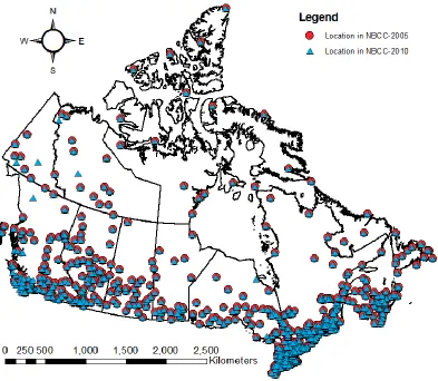
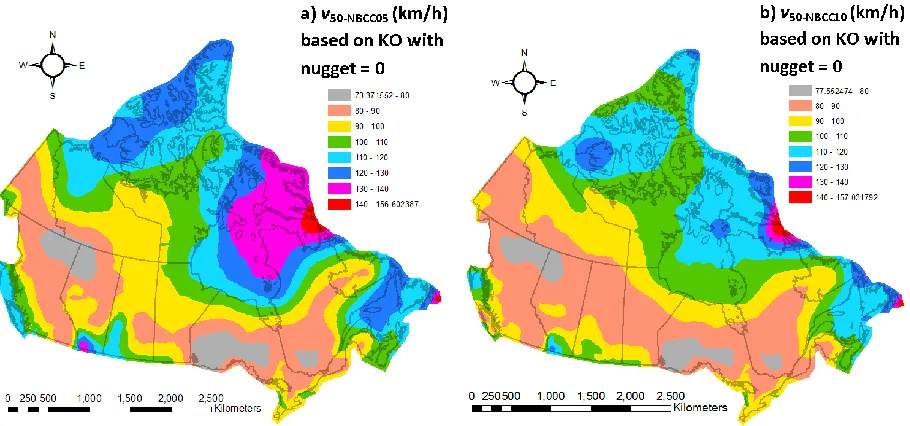
Figure 2.1 Locations tabulated in NBCC-2005 and NBCC-2010. 23

Figure 2.2 Interpolated surfaces based on v50-NBCC05 (In Figure 2.2 to Figure 2.4, v50-NBCC05 and

v50-NBCC10 represent the 50 year return period value of annual maximum wind speed

calculated from the tabulated wind pressure values in NBCC-2005 and NBCC-2010,

respectively.). 24

Figure 2.2 (cont.) Interpolated surfaces based on v50-NBCC05. 25

Figure 2.3 Interpolated surfaces based on v50-NBCC10. 26

Figure 2.3 (cont.) Interpolated surfaces based on v50-NBCC10. 27

Figure 2.4 Interpolated surfaces based on v50-NBCC05 and v50-NBCC10 using the KO with nugget set

equal to 0. 28

Figure 3.1 Locations of the meteorological stations considered in this study. 54

Figure 3.2 Histogram of the years of useable data for each station. 55

Figure 3.3 Histogram of the mean and coefficient of variation of the annual maximum

hourly-mean wind speed for each station. 56

Figure 3.4 Scatter plot of the mean versus of the coefficient of variation of the annual maximum

hourly-mean wind speed. 57

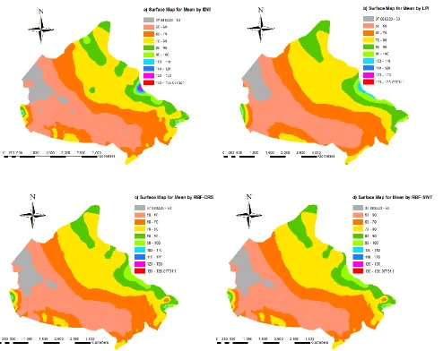
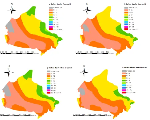
Figure 3.5 Interpolated surfaces of the mean of the annual maximum hourly-mean wind speed

(km/h) using different interpolation methods. 58

Figure 3.5 (cont.) Interpolated surfaces of the mean of the annual maximum hourly-mean wind

(17)

xvi

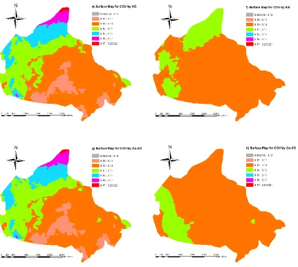
Figure 3.6 Interpolated surfaces of the cov of the annual maximum hourly-mean wind speed

using different interpolation methods. 60

Figure 3.6 (cont.) Interpolated surfaces of the cov of the annual maximum hourly-mean wind

speed using different interpolation methods. 61

Figure 3.7 Interpolated surface of the cov of the annual maximum hourly-mean wind speed using

the GPI. 62

Figure 3.8 Interpolated surfaces of the T-year return period value of the annual maximum

hourly-mean wind speed (km/h) using the RBF-CRS and RBF-SWT. 63

Figure 3.9 Interpolated surfaces of the T-year return period value of the annual maximum

hourly-mean wind speed (km/h) using the KO and Co-KO. 64

Figure 4.1 Meteorological stations considered for the extreme wind speed analysis. 93

Figure 4.2 Histogram of the mean and coefficeint of varaition of the annual maximum

hourly-mean wind speed of each considered station. 94

Figure 4.3 Variation of the L-moment ratios for the considered stations: a) L-cv, b) L-kurtosis

versus L-skewness (The station number is not in any preferred order). 95

Figure 4.4 Dendrogram showing up to 30 nodes along the bottom of the plot considering the

meteorological stations depicted in Figure 4.1 (The node along the horizontal axis represents

a meteorological station or a cluster of meteorological stations; the vertical axis represents

the city block metric distance between two stations or two clusters of stations calculated by

using variables normalized to within 0 to 1 or within -1 to 1.). 96

Figure 4.5 Identified clusters/regions and discordant stations: a) Hierarchical clustering analysis,

(18)

xvii

Figure 4.6 Scatter of the ratio vRE-T/vT for T = 50, 500 and 1000 years (The station number is not

in any preferred order). 98

Figure 4.7 Scatter of the ratio vRG-T/vT for T = 50, 500 and 1000 years (The station number is not

in any preferred order). 99

Figure 4.8 Contour maps of annual maximum wind speed based on vRE-T, vRG-T and vT for T =50,

500 and 1000 years. 100

Figure 5.1 Effect of sample size on 

     _ 

ˆ P_Eˆ(xˆT(ˆ))

E and 

     _ 

SD for the coefficient

of variation of a Gumbel variate X equal to 0.05 and T = 50, 500 and 1000. 126

Figure 5.2 Effect of sample size on the statistics of _ˆ_(  ˆ (ˆ))

L

T W

E x

P and __ˆ(ˆ (ˆ))

H

T E x

P , for the

coefficient of variation of a Gumbel variate X equal to 0.10, αW = 1.4, TL = 50 and TH = 955.

127

Figure 5.3 Effect of sample size on __ˆ



 ˆ (ˆ)

 

/ __ˆ ˆ (ˆ)



H

L T

T

Wx E x

E and



ˆ (ˆ)

 

/ _ˆ ˆ (ˆ)



ˆ   _ 

 W xTL SD xTH

SD for the coefficient of variation of a Gumbel variate X equal

to 0.10, αW = 1.4, TL = 50 and TH = 955. 128

Figure 5.4 Effect of sample size on 

     _ 

E and 

     _ 

SD for k of the GEVD

equal to -0.1 and -0.26, the coefficient of variation of 0.10 and, T = 50, 500 and 1000. 129

Figure 5.5 Effect of sample size on the statistics of _ˆ_(  ˆ (ˆ))

L

T W

E x

P and __ˆ(ˆ (ˆ))

H

T E x

P for the

model parameter k of the GEVD equal to -0.1 and -0.26, the coefficient of variation of 0.10,

αW = 1.4, TL = 50 and TH = 955. 130

Figure 5.6 Estimated Pf based on current NBCC-2010 code design requirements (i.e., αW equal

(19)

xviii

effect; b) Effect of n and RW/D on Pf; c) Effect of n and vX on Pf; d) Effect of n and RW/D on

the standard deviation of __ˆ( (ˆ_T(ˆ))0)

f g x

P ; e) Effect of n and vX on the standard deviation

of _ˆ_( (ˆ_T(ˆ))0)

f g x

P . 131

Figure 5.7 Estimated Pf considering αW equal to 1.0 and use the equivalent TH (i.e., TH = 955,

500 and 295 years for vX equal to 0.1, 0.138 and 0.2 to select the reference wind pressure): a)

Without sample size effect; b) Effect of n and RW/D on Pf; c) Effect of n and vX on Pf; d)

Effect of n and RW/D on the standard deviation of P_f __ˆ(g(xˆT(ˆ))0); e) Effect of n and vX

on the standard deviation of P_f__ˆ(g(xˆT(ˆ))0). 132

Figure 5.8 Estimated Pf considering αW equal to 1.0 and TH equal to 500 and 700 years: a)

Without statistical uncertainty and TH = 500 years; b) Effect of n and RW/D on Pf for TH =

500 years; c) Effect of n and vX on Pf for TH = 500 years; d) Without statistical uncertainty

and TH = 700 years; e) Effect of n and RW/D on Pf for TH = 700 years; f) Effect of n and vX

(20)

xix

LIST OF NOTATIONS

IN CHAPTER 2:

) , ( 0 0 ~

y x

Z = the predicted value at the unmeasured point (x0,y0)

) , (x_i y_i

Z = the measured value at the sample point (x_i,y_i)

i

w = the weight assigned to the sample point (x_i,y_i)

n = the number of sample points considered in the prediction

v50-NBCC05 = the 50-year return period value of annual maximum wind speed calculated from

the tabulated wind pressure values in NBCC-2005

v50-NBCC10 = the 50-year return period value of annual maximum wind speed calculated from

the tabulated wind pressure values in NBCC-2010

IN CHAPTER 3:

T = return period

mvo = the observed mean of the wind speed at a meteorological station

vvo = the observed coefficient of variation of the wind speed at a meteorological station

v = the wind speed

F(v) = the cumulative distribution function of the wind speed which follows the Gumbel

distribution

a = the scale parameter of the Gumbel distribution

u = the location parameter of the Gumbel distribution

(21)

xx

vTo = the observed T-year return period value of the wind speed at a meteorological station

vT(.) = the function of the T-year return period value of the wind speed at a meteorological

station with respect to the term(s) inside the parenthesis

vTs = the interpolated (estimated) T-year return period value of the wind speed

mvs = the estimated mean of the wind speed at one meteorological station

vvs = the estimated coefficient of variation of the wind speed at one meteorological station

σmvs = the standard error of mvs

σvvs = the standard error of vvs

vTsp = the estimated value of the T-year return period value of the wind speed

σTsp = the standard error of vTsp

vo T m v  

= the first derivative of vT with respect to mvo evaluated at mvs

vo T v v  

= the first derivative of vT with respect to vvo evaluated at vvs

2 2 vo T m v  

= the second derivative of vT with respect to mvo evaluated at mvs

2 2 vo T v v  

= the second derivative of vT with respect to vvo evaluated at vvs

IN CHAPTER 4:

λr = the r-th L-moment of the wind speed

τ = the L-coefficient of variation of the wind speed

τ3 = the L-skewness of the wind speed

(22)

xxi lr = the unbiased estimator of λr

bi = the parameters used to calculate lr

n = the size of a set of random sample

xj:n = the j-th ordered sample (in ascending order) of a set of random sample of size n

t = the biased estimator of τ

t3 = the biased estimator of τ3

t4 = the biased estimator of τ4

NTC = the total number of clusters (regions)

N = the total number of the stations or sites within one cluster (region)

ni = the number of the samples considered for the i-th station or site

F = the nonexceedance probability

Qi(F) = the quantile of the nonexceedance probability F

q(F) = the regional quantile of the nonexceedance probability F

μi = the scaling factor taken to be the mean value for the i-th station

Di = the discordancy measure for the i-th station (or site)

ti = the biased estimator of τ for the i-th station (or site)

t3,i = the biased estimator of τ3 for the i-th station (or site)

t4,i = the biased estimator of τ4 for the i-th station (or site)

ui =



ti t3,i t4,i



u = the mean value of ui

S = the sample covariance matrix

H = the heterogeneity measure

(23)

xxii

μV = the mean of the dispersion measure V

σV = the standard deviation of the dispersion V

t = the regional average L- coefficient of variation with stations weighted proportionally to

their record lengths

3

t = the regional average L- skewness with stations weighted proportionally to their record

lengths

4

t = the regional average L- kurtosis with stations weighted proportionally to their record

lengths

) (x

F = the cumulative distribution function of the kappa distribution

κ = the parameter of the kappa distribution

α = the parameter of the kappa distribution

h = the parameter of the kappa distribution

ξ = the parameter of the kappa distribution

) (x

F_G = the cumulative distribution function of the Gumbel distribution

) (x

F_GE = the cumulative distribution function of the generalized extreme value distribution

X = the random variable

x = the specific value of the random variable X

a = the scale parameter of the Gumbel distribution and the generalized extreme value

distribution

u = the location parameter of the Gumbel distribution and the generalized extreme value

distribution

k = the parameter of the generalized extreme value distribution

Dist

(24)

xxiii

Dist

Z₄ = the goodness-of-fit measure based on the L-kurtosis

σ3 = the standard deviation of the regional average L-skewness

σ4 = the standard deviation of the regional average L-kurtosis

vRE-T = the T-year return period value of the annual maximum wind speed obtained based on

the regional frequency analysis and using the generalized extreme value distribution

vRG-T = the T-year return period value of the annual maximum wind speed obtained based on

the regional frequency analysis and using the Gumbel distribution

vT = the T-year return period value of the annual maximum wind speed obtained based on

the at-site analysis and using the Gumbel distribution

IN CHAPTER 5:

T = the return period

FGU(x;θ) = the cumulative distribution function of the Gumbel distribution

FGE(x;θ) = the cumulative distribution function of the generalized extreme value

distribution

) ; ( 

F = FGU(;) for the Gumbel distribution; = FGE(;) for the generalized extreme

value distribution

a = the scale parameter of the Gumbel distribution and the generalized extreme value

distribution

u = the location parameter of the Gumbel distribution and the generalized extreme value

distribution

(25)

xxiv

θ = (u, a) for the Gumbel distribution; = (u, a, k) for the generalized extreme value

distribution

X = the random variable representing the annual maximum hourly-mean wind speed

x = the specific value of the random variable X

vX = the coefficient of variation of the random variable X

μX = the mean of the random variable X

σX = the standard deviation of the random variable X

xT = the T-year return period value of the random variable X

T

xˆ = the estimator of the T-year return period value xT

ˆ = the estimator of θ

) ˆ ( ˆT 

x = the same as xˆ , but to emphasize the uncertainty in _T xˆ is due to the uncertainty in the _T

estimated parameters ˆ

)) ˆ ( ˆ ( ˆ   T E x

P = the probability that the estimated xˆT(ˆ) being exceeded

)) ˆ ( ˆ ( _T 

E x

P = the expected value of __ˆ(ˆ_T(ˆ))

E x P ) ˆ ( ˆ  

f = the joint probability distribution of the estimated distribution parameters ˆ

 



ˆ

E = the expectation of the item inside the parenthesis over ˆ

) (

ˆ 



SD = the standard deviation of the item inside the parenthesis over ˆ

TL = a low return period

L

T

x = the return period value of the wind speed corresponding to the return period TL

αW = the wind load factor

(26)

xxv H

T

x = the return period value of the wind speed corresponding to the return period TH

) ˆ ( ˆ  L T

x = the estimator of

L

T

x , but to emphasize the uncertainty in

L

T

xˆ is due to the

uncertainty in the estimated parameters ˆ

) ˆ ( ˆ  H T

x = the estimator of

H

T

x , but to emphasize the uncertainty in

H

T

xˆ is due to the

uncertainty in the estimated parameters ˆ

(uˆ , aˆ) = the estimator of (u, a)

n = the sample size

50

x = the 50-year return period value of wind speed

R = the random variable representing the resistance

Rn = the nominal resistance

D = the random variable representing the dead load

Dn = the nominal dead load

W = the random variable representing the wind load effect

Z = the random variable representing the transformation factor

Wn = the nominal wind load

) (xT

g = the limit state function by considering the dead and wind loads alone

γR = the resistance factor

αD = the dead load factor

RW/D = the ratio of the factored design wind load to the factored design dead load

XR = R/Rn

XD = D/Dn

(27)

xxvi

) 0 )) ˆ ( ˆ ( (

ˆ  

 T

f g x

P = the probability of g(xˆT(ˆ))0considering the statistical uncertainty in

) ˆ ( ˆT 

x which is caused by the uncertainty in the estimated parameters ˆ

) 0 )) ˆ ( ˆ (

( T  

f g x

P = the expected value of P_f__ˆ(g(xˆT(ˆ))0) over ˆ

Pf = the simplified notation of Pf(g(xT) ≤ 0) or Pf (g(xˆT(ˆ))0)

β = the reliability index

Φ-1

(28)

1

Chapter 1 INTRODUCTION

1.1 Introduction

Wind load is an important factor in the design of engineered structures. It usually deals with the

strongest winds or extreme wind speeds that occur during the lifetime of the structure.

Codification of wind load for structural design requires the estimation of the quantiles or return

period values of the extreme wind speed. In the National Building Code of Canada (NBCC), the

extreme wind speed of interest represents the annual maximum of the moving average (AMMA)

of the 60-minute mean (i.e., hourly-mean) wind speed at a 10 m height in open country terrain, a

standard condition used in the NBCC (NRCC 2010). Unless otherwise indicated, in the

remaining part of this thesis the wind speed refers to the hourly-mean wind speed defined in the

previous sentence.

The extreme wind speeds are estimated based on the measured wind records at different

meteorological stations. However, it is unrealistic to set up meteorological stations everywhere.

For sites which are not covered by the measured values at meteorological stations, the statistics

and quantiles of the annual maximum hourly-mean wind speed could be spatially interpolated

from those measured. Although there are various spatial interpolation methods including the

deterministic methods and the geostatistical methods (Isaaks and Srivastava 1989, Cressie 1993,

Goovaerts 1997, Chiles and Delfiner 1999), it is difficult to draw a general conclusion indicating

which method convincingly outperforms the others because the adequacy of the methods is data

(29)

2

applications of spatial interpolation methods to climatic data deal with rainfall, relative humidity,

solar radiation and temperature (Apaydin et al. 2004). Luo et al. (2008) conducted a comparison

of seven interpolation methods for estimating the daily mean wind speed surface from data

across England and Wales. However, their observations may not be translated to other regions or

extreme values of the climatic data since their analysis was focused on average values of the

climatic data.

In this thesis, 14 different spatial interpolation methods are applied to the 50-year return period

value of the annual maximum hourly-mean wind speed tabulated in the last two versions of

NBCC (i.e. NBCC-2005 and NBCC-2010) as well as the at-site extreme value analysis results

from 235 meteorological stations (each station, except three stations, with more than 20 years of

useable data) in Canada. The preferred method(s) which can produce the best predictions for the

statistics and quantiles of the extreme wind speed are determined based on the (leave-one-out)

cross validation results.

As mentioned above, the statistics and quantiles of the extreme wind speed could be estimated

based on the at-site analysis of the annual maximum wind speed using records at different

meteorological stations. One possible limitation of such an at-site analysis of the annual

maximum wind speed is the insufficient historical wind records at the meteorological stations

because the scarcity of the useable historical data will cause the uncertainty in the estimated

quantiles. To overcome the problem with data deficiency, the “superstation” approach (Peterka

and Shahid 1998), regional frequency analysis (Hosking and Wallis 1997) or pooled frequency

(30)

3

method advocated by Hosking and Wallis (1997) is adopted to estimate the quantiles of the

annual maximum wind speed for Canada by using wind records from 235 meteorological

stations.

Given a specified or nominal wind load, the wind load factor is calibrated based on structural

reliability theory for selected target reliability indices (Madsen et al. 2006). In both NBCC-2005

and NBCC-2010, the 50-year return period value of the annual maximum hourly-mean wind

speed to calculate the nominal wind load and a wind load factor of 1.4 are adopted to achieve a

(50-year) target reliability index of 3.0 (i.e., failure probability of 1.35×10-3) (Bartlett et al. 2003a,

b). It should be noted that the combination of the nominal wind load and the load factor is not

unique because the selection of the return period to specify the wind speed or the reference wind

velocity pressure is not unique. The same target reliability is achieved as long as the factored

design wind load remains the same. However, as mentioned above, the annual maximum wind

records used to calculate the distribution model parameters of the annual extreme wind speed are

often limited, resulting in the estimated distribution model parameters to be uncertain. This

uncertainty can affect the calculated quantile or return period value of the wind speed as well as

the structural reliability. Therefore, with the statistical uncertainty in the probability distribution

model or its parameters for the annual maximum wind speed, two different approaches need to

be investigated for specifying the factored design wind load: a single set of low return period for

the specified wind speed combined with a wind load factor greater than 1.0 versus a single high

return period for the specified wind speed combined with a wind load factor of unity. The

selection of the optimal strategy is significant especially for a region or a country with spatially

(31)

4

1.2 Objectives

The present study is focused on the spatial variation and interpolation of the statistics of the

annual maximum hourly-mean wind speed and its implication in design wind load. The main

objectives are:

1) To select the preferred methods for interpolating the 50-year return period value of the

annual maximum hourly-mean wind speed tabulated in NBCC-2005 and NBCC-2010.

2) To select the preferred methods for interpolating the mean, coefficient of variation and

quantiles of the annual maximum hourly-mean wind speed in Canada and to investigate

the performance of different approaches in estimating the T-year return period value of

the wind speed.

3) To apply the regional frequency analysis method to estimate the quantiles of the annual

maximum wind speed for Canada and compare the results with those based on the at-site

analysis.

4) To investigate the influence of the limited sample size on the calibration of design wind

load and to select an optimal combination of the return period and the load factor for

specifying the wind load in codified design.

1.3 Organization of the thesis

Chapter 2 of this thesis discusses the spatial interpolation of the 50-year return period value of

the annual maximum hourly-mean wind speed tabulated in NBCC-2005 and NBCC-2010. 14

interpolation methods including both the deterministic methods and the geostatistical methods

(32)

5

the (leave-one-out) cross-validation analysis. Discussions and recommendations based on the

cross-validation results are provided for practical applications as well.

Chapter 3 is focused on the spatial interpolation of the statistics (i.e., mean and coefficient of

variation) and quantiles of the annual maximum hourly-mean wind speed in Canada. The

extreme wind records from 235 meteorological stations (each station, except three stations, with

more than 20 years of useable data) in Canada are considered. Similar to Chapter 2, 14

interpolation methods including deterministic methods and geostatistical methods are applied

and the (leave-one-out) cross-validation statistical analysis is carried out in order to compare the

performance of the considered methods. Following that, two possible approaches in estimating

the T-year return period value of the wind speed are considered: 1) directly interpolate it from T

-year return period value of the wind speeds at the meteorological stations, and 2) calculate it

using the mean and coefficient of variation (cov) of the extreme wind speed that are interpolated

from those obtained at meteorological stations. A comparison is conducted to investigate

whether the latter is an accurate substitute for the former.

Chapter 4 applies the regional frequency analysis method to estimate the quantiles of the annual

maximum wind speed for Canada. The same data used in Chapter 3 is considered in the analysis.

Potential homogeneous regions for the extreme wind speeds are identified by using three

different clustering methods (i.e. k-means clustering, hierarchical clustering and self-organizing

map clustering). The regional frequency analysis and statistical tests are then applied to the

identified regions. Quantiles of the annual maximum wind speed are estimated based on the

(33)

6

Potential implications of using the regional analysis results versus the at-site analysis results in

developing the wind hazard maps which are important for the development of codified structural

design are discussed.

Chapter 5 presents the influence of the limited sample size on the calibration of design wind load

and the evaluation of the optimal strategy for specifying the factored design wind load by using

the Monte Carlo technique. The two considered strategies are: a single set of low return period

for the specified wind speed combined with a wind load factor greater than 1.0 versus a single

high return period for the specified wind speed combined with a wind load factor of unity (e.g.,

the approach adopted in the NBCC versus the approach adopted in ASCE-7-10). The optimum is

judged based on the reliability consistency for a realistic range of the coefficient of variation of

the annual maximum wind speed, and the ratio of the design wind load to the design dead load.

Finally, in Chapter 6, the major conclusions of this thesis are summed up and the

recommendations for practical applications and future research are given as well.

1.4 Format of the thesis

This thesis is prepared in a manuscript format as specified by the School of Graduate and

Postdoctoral Studies at the University of Western Ontario. Each chapter, except Chapters 1 and 6,

(34)

7

References

Apaydin, H., Sonmez, F.K. and Yildirim, Y.E. 2004. Spatial interpolation techniques for climate

data in the GAP region in Turkey, Climate Research, 28: 31–40.

Bartlett, F.M., Hong, H.P. and Zhou, W. (2003). Load factor calibration for the proposed 2005

edition of the National Building Code of Canada: Statistics of loads and load effects,

Canadian Journal of Civil Engineering, 30(2): 440-448.

Bartlett, F.M., Hong, H.P. and Zhou, W. (2003). Load factor calibration for the proposed 2005

edition of the National Building Code of Canada: Companion-action load combinations,

Canadian Journal of Civil Engineering, 30(2): 429-439.

Chiles, J. and Delfiner, P. 1999. Geostatistics-modeling spatial uncertainty. John Wiley & Sons,

New York, NY, USA.

Cressie, N. 1993. Statistics for spatial data. John Wiley & Sons, New York, NY, USA.

Goovaerts, P. 1997. Geostatistics for natural resources evaluation. Oxford University Press,

New York, NY, USA.

Hosking, J.R.M. and Wallis, J.R. (1997). Regional frequency analysis: an approach based on

L-moments, Cambridge University Press, Cambridge, UK.

Isaaks, E.H. and Srivastava, R.M. 1989. An introduction to applied geostatistics, Oxford

University Press, New York, NY, USA.

Luo, W., Taylor, M.C. and Parker, S.R. 2008. A comparison of spatial interpolation methods to

estimate continuous wind speed surfaces using irregularly distributed data from England and

Wales，Int. J. Climatol. 28: 947–959.

Madsen, H. O., Krenk, S., and Lind, N. C. (2006). Methods of structural safety, Dover Ed.,

(35)

8

NRCC (2005). National Building Code of Canada. Institute for Research in Construction,

National Research Council of Canada, Ottawa, Ontario.

NRCC (2010). National Building Code of Canada. Institute for Research in Construction,

Peterka, J. and Shahid, S. (1998). Design gust wind speeds in the United States, Journal of

Structural Engineering, 124: 207–214.

Reed, D.W., Jacob, D., Robson, A.J., Faulkner, D.S., Stewart, E.J. (1999). Regional frequency

analysis: a new vocabulary, in Gottschalk, L., Olivry, J.-C., Reed, Rosbjerg (Eds.),

Hydrological Extremes: Understanding, Predicting, Mitigating, Proceedings of the

(36)

9

Chapter 2 SPATIAL INTERPOLATION OF EXTREME

WIND SPEEDS BASED ON CODE SUGGESTED

VALUES

2.1 Introduction

Nominal wind load is required in structural design and code calibration. In the last two

versions of the National Building Code of Canada (NBCC) (NRCC 2005, 2010), the

nominal design wind load is specified based on the reference wind velocity pressures

which are calculated using the estimated 50-year annual maximum hourly-mean wind

speeds (i.e., the 0.98 quantile of annual maximum hourly-mean wind speed) (NRCC

2010). The extreme wind speeds are estimated based on the wind records at different

meteorological stations, and considering expert opinion. Values are tabulated in

NBCC-2005 for 639 locations and NBCC-2010 for 675 locations. For sites which are not

covered by the tabulated values, the reference wind velocity pressures or the

corresponding 50-year return period values of the wind speed could be spatially

interpolated from those tabulated.

The spatial interpolation methods fall into two categories: 1) deterministic methods and 2)

geostatistical methods (Isaaks and Srivastava 1989, Cressie 1993, Goovaerts 1997, Chiles

and Delfiner 1999). The deterministic methods calculate the predictions from the

measured values (or values at sample points) based on either the extent of similarity or

(37)

10

include the inverse distance weighting, global polynomial interpolation, local polynomial

interpolation, and radial basis functions methods. They have no assessment of errors

associated with the predicted values. Geostatistical methods incorporate the randomness

into the interpolation and use the statistics of the measured values. The commonly used

geostatistical methods are kriging and co-kriging. In addition to predicting values, the

geostatistical methods evaluate the prediction error as well. The spatial interpolation

methods can be either an exact or an inexact interpolator. The exact interpolator provides

an estimated value that is the same as the measured value at a sample point. An inexact

interpolator predicts an estimate that differs from its known value at a sample point.

However, the method which provides the best predictions is usually not clear because the

adequacy of the methods is data dependent and different methods can result in

significantly different interpolated values. A (leave-one-out) cross-validation analysis can

be used to determine the best interpolation method among all potential methods. To

perform the cross-validation analysis, data at one or more measurement locations are

withheld and are predicted using a selected spatial interpolation method with the

remaining samples (Cressie 1993, Johnston et al. 2003); statistics of the differences

between the measured and predicted values obtained for the measurement locations are

evaluated and used as performance indicators.

A review of some of the applications of spatial interpolation methods to climatic data

given by Apaydin et al. (2004) shows that most applications and case studies deal with

(38)

11

difficult to draw a general conclusion indicating which method convincingly outperforms

the others. They applied six spatial interpolation methods to the climatic data of a region

in Turkey, and indicated that completely regularized spline and simple co-kriging are the

preferred methods based on the root mean square error (RMSE) in the cross-validation

analysis. A comparison of seven methods for interpolating the daily mean wind speed

surface from data across England and Wales was conducted by Luo et al. (2008). Their

results show that the co-kriging was most likely to produce the best estimation of a

continuous surface with temporal consistency, and that the co-kriging surfaces reflect the

wind features more accurately, especially in mountain areas, than the kriging surfaces

because of the use of terrain’s elevation as a covariate. However, the above observed

performance of the methods may not be translated to other regions or extreme values of

the climatic data since their analysis was focused on average values of the climatic data.

The present study is focused on the spatial interpolation of the 50-year return period

value (i.e. 0.98 quantile) of the annual maximum hourly-mean wind speed tabulated in

NBCC-2005 and NBCC-2010. The spatial distribution of the tabulated locations in

NBCC-2005 and NBCC-2010 are shown in Figure 2.1. The analysis is aimed at selecting

the preferred method for interpolation of extreme wind speeds. 14 interpolation methods

including both the deterministic methods and the geostatistical methods are employed in

this study. The (leave-one-out) cross-validation analysis was carried out to compare the

performance of the considered methods. Discussions and recommendations based on the

(39)

12

2.2 Spatial interpolation methods used for the numerical analysis

Interpolation methods are used to estimate values for spatially continuous phenomena

from the measured values at limited sample points. Nearly all spatial interpolation

methods are based on the same idea that the estimations are represented as the weighted

averages of the (measured) values at the sample points. The general estimation formula is

depicted as follows:



  n i i i iZ x y

w y x Z 1 0 0 ~ ) , ( ) , ( (2.1)

where ( ₀, ₀)

~

y x

Z represents the predicted value at the unmeasured point (x₀,y₀) ,

) , (xi yi

Z represents the measured value at the sample point (xi,yi), wi is the weight

assigned to the sample point (x_i,y_i), n is the number of sample points considered in the

prediction (Webster and Oliver, 2001). The specific mathematical formulation of each

interpolation methods may have some kind of variation on the general formula depicted

in Eq. (2.1). For example, different interpolation methods may have different ways to

assign the weights for each sample point, or a stationary or nonstationary mean may be

considered to exist among the sample points, or multi-variable instead of one single

variable may be involved. Eight deterministic methods (i.e., inverse distance weighting,

global polynomial interpolation, local polynomial interpolation, and five sub-types of

radial basis functions) and six geostatistical methods (i.e, various kriging and co-kriging)

are used in this study. Some explanations of the methods which are based on Isaaks and

Srivastava (1989), Cressie (1993), Goovaerts (1997), Chiles and Delfiner (1999) and

Johnston et al. (2003) are given below. For more details about the mathematical

(40)

13

described their implementation in ArcGIS that is employed for the numerical analysis in

the following sections.

2.2.1 Deterministic methods

The deterministic methods considered in the present study include the inverse distance

weighting (IDW) method, global polynomial interpolation (GPI) method, local

polynomial interpolation (LPI) method and radial basis functions (RBFs) method.

The IDW is based on a fundamental geographic principle that the observations at near-by

locations are more alike. It calculates the predictions using a linearly weighted

combination of a set of observed values, and the weight is a function of the inverse

distance resulting in a decrease of the influence of the measured location on the predicted

location as the distance increases. The parameter that controls the decrease is optimized

in ArcGIS. Since it is an exact interpolator, the IDW is likely to produce surfaces with

sharp peaks or troughs. It estimates surface values between the maximum and the

minimum of the measured values at sample points.

The GPI method uses a polynomial to fit the observed values and interpolate the surface.

The coefficients of the polynomials are determined by using a least-squares regression to

minimize the residuals. The GPI is an inexact interpolator and the smoothing of the

interpolated surface is determined by the order of the polynomial. The LPI method is

(41)

14

“window” and weights are considered. The coefficients of the polynomials in this case

depend on the moving window.

The RBFs, also known as splines, are exact deterministic interpolators which are

conceptually similar to fit a rubber membrane through measured values while minimizing

the total curvature of the surface. Splines are adequate for surfaces with gentle slopes and

are inadequate for surfaces defined by dataset with large changes within a short

horizontal distance. Unlike the IDW, splines can estimate surface values above the

maximum and below the minimum of the measured values. Five special splines (i.e.,

completely regularized spline (RBF-CRS), spline with tension (RBF-SWT), thin plate

spline (RBF-TPS), multiquadric (RBF-M), inverse multiquadratic (RBF-IM)) available in

ArcGIS are tested since the spline that is best suited to interpolate the extreme wind

speed is unknown.

2.2.2 Geostatistical methods

Unlike the deterministic methods, the geostatistical methods incorporate the concept of

randomness and provide both the predicted surfaces and the assessment of the errors

associated with the predicted values. The geostatistical methods employed in this study

are the kriging and co-kriging. Similar to the IDW, kriging uses a linear combination of

weighted measured values to generate estimates for unmeasured locations. However, the

weights in kriging are based not only on the distance between the measured locations and

the predicted location, but also on the spatial correlation (i.e., semi-variogram) of the

(42)

15

distance or directional bias exists in the data. Co-kriging is similar to kriging, except that

it incorporates additional covariates and the correlations among different variables.

Co-kriging can be effective for data with significant inter-variable correlation. In this study,

since the extreme wind speed could be affected by the terrain’s elevation, the

interpolation may be improved by using co-kriging with the terrain’s elevation at the

meteorological station as a covariate, which will be discussed in the next section.

Three different types of kinging and three different types of co-kriging (i.e., the ordinary

kriging (KO), simple kriging (KS), universal kriging (KU), ordinary co-kriging (CoKO),

simple co-kriging (CoKS), universal co-kriging (CoKU)) with spherical model for the

semi-variogram are used in the present study. The KO assumes that the interpolated

surface has an unknown but constant mean. The weights are determined based on the

minimization of the variance of the error of the prediction. The KS and KU are similar to

the KO, except that the KS assumes that the mean of the surface is a known constant; the

KO assumes that there is a trend in the local mean of the surface which can be defined by

a deterministic function.

2.3 Analysis results

2.3.1 Interpolated surfaces for the 50-year return period value of wind speed

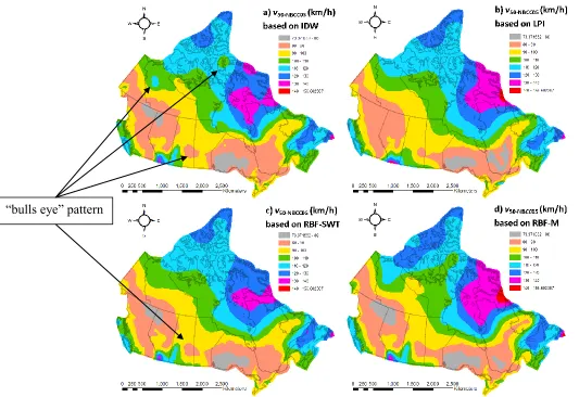
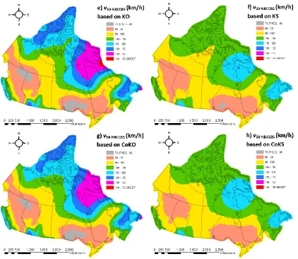
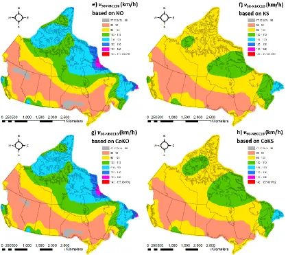
Some interpolated surfaces of the 50-year return period value of wind speed by using

IDW, LPI, RBF-SWT, RBF-M, KO, KS, CoKO, and CoKS are illustrated in Figure 2.2

(43)

16

respectively. The surfaces generated by other interpolation methods are not included

because they produce very similar results or lead to relatively large RMSE. A comparison

of Figure 2.2 and Figure 2.3 shows that the interpolated surfaces based on NBCC-2010

are smoother than those based on NBCC-2005. In Figure 2.2, typical “bulls eye” patterns

can be observed from the surfaces interpolated by using the IDW as well as those by

using the RBF-SWT and RBF-M but with a lesser degree. This is expected because the

IDW, RBF-SWT and RBF-M are exact interpolators. Geostatistical methods, especially

the KS and CoKS, have significant smearing effect on the interpolated surfaces. In Figure

2.3Error! Reference source not found., the “bulls eye” pattern still exists in the

surfaces obtained by using the IDW and M; the surface obtained by using the

RBF-SWT does not exhibit that much of this pattern. Again, the use of the KS and CoKS

results in much smoother surfaces than others. In both Figure 2.2 and Figure 2.3, the

surfaces interpolated by using the kriging and co-kriging look pretty similar indicating

that there is no strong correlation between the extreme wind speed and the terrain’s

elevation.

It is noteworthy that the KO can be an exact interpolator by setting the nugget value equal

to zero. The interpolated surfaces obtained using the KO with zero nugget are depicted in

Figure 2.4. It can be observed that the smearing effect of the KO with nonzero nugget

was reduced and the “bulls eye” pattern starts to appear (especially on the surface based

(44)

17 2.3.2 Cross-validation statistics for the interpolated surfaces of the 50-year return

period value of wind speed

To determine the preferred interpolation methods, the cross-validation analysis was

carried out for the 14 considered spatial interpolation methods and the results are

tabulated in Table 2.1 and Table 2.2 for deterministic methods and geostatistical methods,

respectively. Statistics from the cross-validation for deterministic methods include the

mean of the prediction error (ME) and the RMSE. The method which produces the lowest

RMSE value and/or the ME value close to zero (i.e., least biased model) is considered as

the preferred one. It is observed from Table 2.1 that for NBCC-2005, the preferred

deterministic method to interpolate the 50-year return period value of wind speed is the

RBF-M. This preference is followed by the RBF-SWT, IDW, and RBF-CRS. For

NBCC-2010, the RBF-M, and IDW, providing similar ME and RMSE values, are the preferred

deterministic methods which are followed by the RBF-SWT, and RBF-CRS.

Besides the ME and RMSE, the statistics from the cross-validation analysis for the

geostatistical methods include the average standard error (ASE), the mean of

standardized prediction errors (M-SE), root mean square standardized prediction errors

(RMS-SE) (Johnston et al. 2003). As mentioned earlier, the geostatistical methods

provide predictions as well as the assessment of prediction standard errors. The ASE is

defined as the mean of the prediction standard errors; the standardized prediction error is

equal to the prediction error divided by the prediction standard error. The preferred

geostatistical method is selected based on the lowest RMSE, and/or RMS-SE close to one.

(45)

18

CoKO, is the preferred geostatistical methods for the 50 year return period value of wind

speed in NBCC-2005. The KS and CoKS, although giving smoother interpolated surfaces

than others, produce high RMSE values, and RMS-SE far away from one, therefore

cannot be considered as suitable for interpolating the extreme wind speeds in the present

study. The same results are shared for the 50 year return period value of wind speed in

NBCC-2010.

A comparison of the results in Table 2.1 and Table 2.2 indicates that for NBCC-2005, if

only the RMSE is considered, all the preferred deterministic methods including the

RBF-M, RBF-SWT, IDW and RBF-CRS are superior to the preferred geostatistical method –

the CoKO; the RBF-M, RBF-SWT and IDW also outperform the preferred geostatistical

method – the KO. For NBCC-2010, the preferred deterministic methods such as the

RBF-M and IDW outperform both the KO and CoKO, while other preferred deterministic

methods such as the RBF-SWT and RBF-CRS are considered to provide similar results

as the KO and CoKO.

2.4 Conclusion

The quantiles of the annual maximum hourly-mean wind speed tabulated in NBCC-2005

and NBCC-2010 are only for limited locations. For sites which are not covered by the

code values, spatial interpolation is required to estimate the quantiles of the extreme wind

speed. The present study is focused on the selection of the preferred method for spatially

interpolating the 50-year return period value of the annual maximum hourly-mean wind

(46)

19

been applied to the data tabulated for 639 locations in NBCC-2005 and 675 locations in

NBCC-2010. The interpolated surfaces and the statistics of the cross-validation analysis

indicate that for both NBCC-2005 and NBCC-2010, the RBF-M is the preferred

deterministic method and the KO is the preferred geostatistical method. The RBF-SWT,

RBF-CRS, and IDW produce comparable results as the RBF-M; the CoKO produces

comparable results as the KO. The KS and CoKS generate surfaces with significant

smearing effect. If the selection is based only on the RMSE value, the RBF-M

outperforms the KO.

References

Apaydin, H., Sonmez, F.K. and Yildirim, Y.E. 2004. Spatial interpolation techniques for

climate data in the GAP region in Turkey, Climate Research, 28: 31–40.

Chiles, J. and Delfiner, P. 1999. Geostatistics-modeling spatial uncertainty. John Wiley

& Sons, New York, NY, USA.

Cressie, N. 1993. Statistics for spatial data. John Wiley & Sons, New York, NY, USA.

Goovaerts, P. 1997. Geostatistics for natural resources evaluation. Oxford University

Press, New York, NY, USA.

Isaaks, E.H. and Srivastava, R.M. 1989. An introduction to applied geostatistics, Oxford

University Press, New York, NY, USA.

Johnston, K., Ver Hoef, J.M., Krivoruchko, K. and Lucas, N. 2003. ArcGIS 9, Using

ArcGIS Geostatistical Analyst, Redlands, CA: Environmental Systems Research

(47)

20

Luo, W., Taylor, M.C. and Parker, S.R. 2008. A comparison of spatial interpolation

methods to estimate continuous wind speed surfaces using irregularly distributed data

from England and Wales，Int. J. Climatol. 28: 947–959.

NRCC. 2005. National Building Code of Canada. Institute for Research in Construction,

NRCC. 2010. National Building Code of Canada. Institute for Research in Construction,

Webster, R. and Oliver, M. 2001. Geostatistics for Environmental Scientists. John Wiley

(48)

21

Table 2.1 Statistics from the cross-validation analysis for deterministic methods.

Methods

50-year return period value of wind speed in

NBCC-2005

50-year return period value of wind speed in

NBCC-2010

ME (km/h) RMSE(km/h) ME (km/h) RMSE(km/h) IDW -1.82E-01 5.49 -1.88E-02 5.39

GPI 2.67E-02 11.16 1.80E-02 8.84 LPI 2.20E-01 6.33 1.72E-01 6.03

RBFs

(49)

22

Table 2.2 Statistics from the cross-validation analysis for geostatistical methods.

Methods

50-year return period value of wind speed in NBCC-2005

50-year return period value of wind speed in NBCC-2010

ME (km/h)

RMSE (km/h)

ASE

(km/h) M-SE

RMS-SE

ME (km/h)

RMSE (km/h)

ASE

(km/h) M-SE

(50)

23

(51)

24

Figure 2.2 Interpolated surfaces based on v50-NBCC05 (In Figure 2.2 to Figure 2.4, v50-NBCC05 and v50-NBCC10 represent the 50 year return

period value of annual maximum wind speed calculated from the tabulated wind pressure values in NBCC-2005 and NBCC-2010,

(52)

25

(53)

26

(54)

27

(55)

28

(56)

29

Chapter 3 COMPARISON OF SPATIAL INTERPOLATION

TECHNIQUES FOR EXTREME WIND SPEEDS OVER

CANADA

3.1 Introduction

Specified extreme wind speed or its corresponding wind velocity pressure is tabulated in

structural design codes and used for design. Statistical methods and probabilistic models

used to estimate the wind speed for Canadian design code were presented by Yip et al.

(1995). Models and techniques used to estimate the quantiles of the extreme wind speed

for other countries and regions were presented, among others, by Peterka and Shahid

(1998), Holmes and Moriarty (1999), Palutikof et al. (1999), Simiu et al. (2001), Sacre

(2002), Kasperski (2002), and Harris (2005). The estimated extreme wind speed

represents those at the sites where the wind speeds are recorded. The specified values in

the 2010 version of the National Building Code of Canada (NBCC) are based on 50-year

return period value of annual maximum hourly-mean wind speed (i.e., the 0.98 quantile

of annual maximum hourly-mean wind speed) (NRCC 2010). The values tabulated in the

code for many locations are spatially interpolated from the extreme value analysis results

of wind records at the meteorological stations. The interpolation is partly based on expert

opinion. Furthermore, statistical characteristics of the annual maximum wind speed,

including the mean and coefficient of variation (cov), are needed to evaluate the

structural reliability (Madsen et al. 2006). The statistics can be spatially interpolated for

Spatial Variation and Interpolation of Wind Speed Statistics and Its Implication in Design Wind Load

Scholarship@Western

Scholarship@Western

Spatial Variation and Interpolation of Wind Speed Statistics and

Spatial Variation and Interpolation of Wind Speed Statistics and

Its Implication in Design Wind Load

Its Implication in Design Wind Load

ABSTRACT

CO-AUTHORSHIP

ACKNOWLEDGEMENTS

TABLE OF CONTENTS

LIST OF TABLES

LIST OF FIGURES



 





 



LIST OF NOTATIONS

IN CHAPTER 2:

IN CHAPTER 3:

IN CHAPTER 4:





IN CHAPTER 5:

 

Chapter 1

INTRODUCTION

1.1

Introduction

1.2

Objectives

1.3

Organization of the thesis

1.4

Format of the thesis

References

Chapter 2

SPATIAL INTERPOLATION OF EXTREME

WIND SPEEDS BASED ON CODE SUGGESTED

VALUES

2.1

Introduction

2.2

Spatial interpolation methods used for the numerical analysis



2.3

Analysis results

2.4

Conclusion

References

Chapter 3

COMPARISON OF SPATIAL INTERPOLATION

TECHNIQUES FOR EXTREME WIND SPEEDS OVER

CANADA

3.1

Introduction